Anomalous sensitivity to initial conditions and entropy production in standard maps: Nonextensive approach
Abstract
We perform a throughout numerical study of the average sensitivity to initial conditions and entropy production for two symplectically coupled standard maps focusing on the control-parameter region close to regularity. Although the system is ultimately strongly chaotic (positive Lyapunov exponents), it first stays lengthily in weak-chaotic regions (zero Lyapunov exponents). We argue that the nonextensive generalization of the classical formalism is an adequate tool in order to get nontrivial information about this complex phenomenon. Within this context we analyze the relation between the power-law sensitivity to initial conditions and the entropy production.
PACS number: 05.45.-a, 05.20.-y, 05.45.Ac.
I Introduction
Hamiltonian chaotic dynamics is related to the description of irregular trajectories in phase space. This characteristic is closely linked to the instability of the system and the entropy growth (see, e.g., ott ). Chaotic dynamics is in fact associated with positive Lyapunov coefficients, which corresponds, through the Pesin equality pesin , to a positive Kolmogorov-Sinai entropy rate kolsinai . However, many physical, biological, economical and other complex systems exhibit more intricate situations, associated to a phase space that reveals complicated patterns and anomalous, not strongly chaotic, dynamics gell_mann_01 . In many of these cases, the system displays an algebraic sensitivity to initial conditions and the use of the Boltzmann-Gibbs (BG) entropic functional for the definition of quantities such as the Kolmogorov-Sinai entropy rate only provides trivial information. It has been first argued tsallis_01 , then numerically exhibited Costa_Lyra_Plastino_CT ; Lyra_CT ; Latora_Baranger_Rapisarda_CT ; Tirnakli_Ananos_CT ; ernesto , and finally analytically shown baldovin_01 ; baldovin_02 that under these conditions the nonextensive generalization tsallis_02 of the BG entropic form adequately replaces these concepts. This generalization has been successfully checked for many cases where long-range interactions, long-range microscopic memory, some kind of fractalization of the phase space are inherent. Indeed, in the case of one-dimensional dissipative maps, following pioneering work grassberger_01 on asymptotic algebraic sensitivity to initial conditions, it has been numerically tsallis_01 ; Costa_Lyra_Plastino_CT ; Lyra_CT ; Latora_Baranger_Rapisarda_CT ; Tirnakli_Ananos_CT ; ernesto and analytically proved baldovin_01 that the nonextensive formalism provides a meaningful description of the critical points where the Lyapunov coefficient vanishes. Moreover, through the nonextensive entropy it is possible to prove a remarkable generalization of the Pesin equality baldovin_02 .
On the basis of these results, we present here a nonextensive approach to the description of complex behaviors associated to Hamiltonian systems that satisfy the Kolmogorov-Arnold-Moser (KAM) requirements (see, e.g., zaslavsky_01 ). The phase space consists in this case of complicated mixtures of invariant KAM-tori and chaotic regions. A chaotic region is in contact with critical KAM-tori whose Lyapunov coefficients are zero, and a chaotic orbit sticks to those tori repeatedly with a power-law distribution of sticking times (see, e.g., zaslavsky_02 and references therein). It is known that, under these conditions, one main generic characteristic feature of Hamiltonian chaos is its nonergodicity, due to the existence of a finite measure of the regularity islands area. The set of islands is fractal, and thin strips near the islands’ boundary, which are termed boundary layers, play a crucial role in the system dynamics. In addition to these processes, there are effects that arise solely because of the high enough dimensionality of the system. One of these effects is Arnold diffusion arnold , that occurs if the number of degrees of freedom of the Hamiltonian system is larger than two ott ; zaslavsky_01 . In general, for the usual case of many-body short-range-interacting Hamiltonian systems, the combination of these nonlinear dynamical phenomena typically makes the system to leave the generic situation of nonergodicity and eventually yields ergodicity.
Along these lines, anomalous effects for the sensitivity to initial conditions and for the entropy production have already been investigated within the nonextensive formalism baldovin_03 for a paradigmatic model that exhibits the KAM structure, namely the well known standard map chirikov_01 . In the present paper we focus on two symplectically coupled standard maps. The choice of two coupled maps is because this is the lowest possible dimension () of Hamiltonian maps where Arnold diffusion does take place, an effect that has a fundamental impact for the macroscopic effects associated with the dynamics of the system, since it guarantees an unique (connected) chaotic sea (see, e.g., baldovin_04 ; baldovin_05 ).
In Ref. latora_02 it was numerically shown that, for low-dimensional Hamiltonian (hence symplectic) maps, the Kolmogorov-Sinai entropy rate coincides with the entropy produced per unit time by the dynamical evolution of a statistical ensemble of copies of the system that is initially set far-from-equilibrium, i.e., . More precisely, considering an ensemble of copies of the map and a coarse graining partition of the phase space composed by nonoverlapping (hyper)cells (with nonvanishing hypervolumes), at each iteration step a probability distribution is defined by means of the occupation number of each cell, (), and we have that
| (1) |
where the average is taken considering the dynamical evolution of different ensembles, all starting far-from-equilibrium, but with different initial conditions. In this paper, as far-from-equilibrium initial conditions, we will consider an ensemble of copies of the map all randomly distributed inside a single (hyper)cell of the partition. In this way the initial entropy is zero, since all but one probabilities vanish. Averages are then obtained by sampling the whole phase space changing the position of the initial (hyper)cell.
On the other hand, one can consider the sensitivity to initial conditions
| (2) |
that in general depends on the phase space initial position and on the direction in the tangent space . If the system is chaotic, the exponential sensitivity to initial conditions defines a spectrum of Lyapunov coefficients coupled in pairs ( being the phase space dimension), where each element of the pair is the opposite of the other (symplectic structure). By the Pesin identity we have that and the result in latora_02 states then that
| (3) |
where once again stands for average over different initial data.
Now, when the largest Lyapunov coefficient vanishes, Eq. (3) provides only poor information ( , to be precise), which is not useful for distinguishing, for example, between weak chaoticity and regularity. In order to address this issue, we generalize the previous approach in the sense of the nonextensive generalization tsallis_02 of the classical (BG) formalism. Specifically, we define the -generalized entropy production (corresponding to the -generalization of the Kolmogorov-Sinai entropy rate) as
| (4) |
where the nonextensive entropy is defined by
| (5) |
and stands for entropy. In case of equiprobability, i.e., , the nonextensive entropy takes the form , where (with is known in the literature as the -logarithm quimicanova . Notice that its inverse, the -exponential, is given by
| (6) |
In this paper we will show that, in situations where the largest Lyapunov coefficient tends to zero, a regime emerges (that we will discuss in more details later on) where the sensitivity to initial conditions takes the form of a -exponential, namely
| (7) |
with a specific value of the index and of the generalized Lyapunov coefficient ( stands for sensitivity). Correspondingly, a single value of exists for which the generalized entropy (5) displays a regime of linear increase with time. Under these conditions, we study the relation between and . We will see that, differently to what happens in the case of strong chaos (where ), the two indices and do not coincide in general. We discuss the origin of this fact.
II Sensitivity to initial conditions and entropy production
We consider a dynamical system with an evolution law given by two symplectically coupled standard maps:
| (12) |
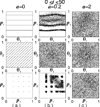
where , can be regarded respectively as an angle and an angular momentum coordinate, , and . Since the system is symplectic , it immediately follows that it also is conservative, i.e., the Jacobian determinant of the map is one (). For the sake of definiteness, most part of this paper will deal with the setting , so that the analysis will be restricted to the case where the system is symmetric with respect to exchange . If the coupling parameter vanishes, the two standard maps decouple. For a generic value of , the system is integrable for , while chaoticity rapidly increases with . For intermediate values of , trajectories in phase space define complex structures. The phase space is non-uniform and consists of domains of chaotic dynamics (stochastic seas, stochastic layers, stochastic webs, etc.) and islands of regular quasi-periodic dynamics zaslavsky_01 . To illustrate these behaviors, in Fig. 1(a-c) we show the projection on various planes of the dynamical evolution of an ensemble of points uniformly distributed in phase space at , for (strong chaos), (weak chaos), and (integrability). Reminding the fact that the shadow of a (fractal-like) sponge on a wall has a regular geometry, the presence of structures as those that appear for in the projection of the ensemble over coordinates planes is a strong hint that even more intricate structures are present in the phase space itself. In order to further characterize the strongly and the weakly chaotic situations, Figs. 2 and 3 display, for different fixed times, the projection of the evolution of an initially out-of-equilibrium ensemble, respectively for and . In all previous figures we have fixed .


Chaotic regions produce exponential separation of initially close trajectories. Before entering in the details of our analysis, let us consider how the usual, strongly chaotic case is described inside the nonextensive formalism, both for the sensitivity to initial conditions and the entropy production. To extract the mean value of the largest Lyapunov coefficient and the mean entropy production rate, we analyze respectively the average values and , over different initial conditions. Fig. 4, when , reproduces the results in latora_02 for , and (strong chaos). Only for both the average logarithm of the sensitivity to initial conditions and the average entropy display a regime with a linear increase with time, before a saturation effect due to the finiteness of the total number of (hyper)cells. If (), the curve is convex (concave) for both quantities. Notice that the slope of the linear increase of is smaller than the slope of , as, since the phase space is -dimensional, there are two positive Lyapunov exponents to be considered in Eq. (3).

We turn now our attention to the weak chaos. Fig. 5 shows that, fixing and decreasing now , the mean value of the largest Lyapunov coefficient tends to zero as a consequence of the fact that dynamics is now more constrained by structures in phase space. Particularly, for an initial phase emerges for which is not linear (see the inset of Fig. 5). We refer to this phase as the weakly chaotic regime. As tends to zero, the crossover time (see its definition in Fig. 6) between this initial regime and the one characterized by a linear increase of increases, so that the weakly chaotic phase becomes more and more important. The sensitivity to initial conditions in correspondence to this initial regime is power-law. In fact, Fig. 7 exhibits that, for specific values , grows linearly during this regime and starts later to be convex when the sensitivity becomes exponential, after the crossover. For approaching zero, the crossover time between this initial regime and the strongly chaotic regime (characterized by a linear increase of ) diverges (see inset of Fig. 7). Note that depends on . For integrability we have, as expected, .


The weakly chaotic regime can also be detected by an analysis of the entropy production, performed as described in section I. In Fig. 8 we take as an example the case and . For the weakly chaotic regime the result is similar to Fig. 4(b), but the value for which the entropy grows linearly is now instead of .

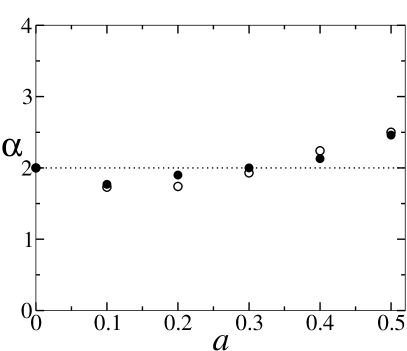
Fig. 9 synthesizes the behavior of and for two different fixed coupling constants, namely and . At variance with what happens in the strongly chaotic regime, in the weakly chaotic one and are not the same. In the next section we discuss the origin of this difference.

Another numerical result is that, while the the generalized Lyapunov coefficient appears to be almost independent from ( and for and respectively), the generalized Kolmogorov-Sinai entropy rate exhibits, within our numerical precision, a slight decrease as increases. We do not have yet a clear explanation for this observation.
III Discussion
To understand the origin of the discrepancy, in the weakly chaotic regime, between and some simple geometric considerations are in order.
Firstly, we notice the following property of the -logarithmic function:
| (13) |
where and , are related by
| (14) |
Notice that, for all , implies , whereas implies .
Secondly, for simplicity, we consider the case of a -dimensional phase space where the dynamical evolution is symmetric with respect to the exchange of the coordinates. Let us call the total number of bidimensional cells composed by a partition of intervals in each coordinate. We suppose to set a far-from-equilibrium initial ensemble inside a single -dimensional cell and that the dynamical evolution of each trajectory in the ensemble implies a spreading of the ensemble in phase space. Let and be respectively the number of occupied -dimensional intervals in one of the two coordinate axes and the number of occupied -dimensional cells, at time (). The relation between and depends on the details of the dynamical evolution. Two limiting cases are
| (15) |
The former is realized for instance when there is a predominant direction along which the ensemble stretches, so that the dynamical evolution of the ensemble produces filaments in the -dimensional phase space and it is essentially unidimensional. The latter happens for example when the dynamical evolution in the two coordinates is decoupled, so that is simply the Cartesian product . Now, if we suppose that , for a specific value of the parameter (we are using the notation consistently with the fact that represents the growth of a unidimensional arc), by means of Eqs. (13) and (14) we have that for the values
| (16) |
respectively, for the two previous limiting cases (in Eq. (11)). Notice that for both cases. Of course, Eq. (12) can be straightforwardly generalized for arbitrary dimensions of the phase space.


This geometrical analysis applies to the problem of the entropy production, strictly speaking, only if the ensemble evolves according to a uniform distribution in phase space (equiprobability), so that the value of the generalized entropy is given by . Nonetheless, we will see now that the same analysis is useful to understand the dynamical behavior of the model that we are studying. We start by considering the effect of the coupling term in the special case , that corresponds to integrability. Fig. 10 represents the behavior of and for this case. As expected, is zero, thus displaying that the sensitivity to initial conditions increases linearly. On the other hand, the behavior of is understood if we analyze in some details the dynamics. We have that and are just conserved along any trajectory and all the interesting dynamical evolution take place in the -plane by means of the iteration laws
| (17) | |||||
As it is apparent, the two coordinates are decoupled and for the growth of the ensemble is -dimensional as confirmed by Fig. 11 (first row). Under these conditions, we have , so that, applying the previous analysis, we obtain . For the maps further degenerates, since now we have one more conserved quantity, i.e.,
| (18) |
This implies (see Fig. 11, second row), and we obtain . Around there is then a transition from to , as it is exhibited in Fig. 10.
We can consider now the generic weakly chaotic case (). In Fig. 12 we estimate the (below defined) factor that connects the -dimensional analysis performed by the entropy to the one-dimensional inspection provided by the sensitivity to initial conditions, by means of the relation (see Eq. (14))
| (19) |
For both and , small positive values of yield , as it is for the integrable case . This exhibits an essentially -dimensional growth of the portion of the phase space occupied by the ensemble.
At this point we can advance a conjecture for the more general case of a phase space that is not symmetric under the interchange of coordinates. This conjecture will allow for a better understanding of the reason of the discrepancy between and . In the case of strong chaos in a symplectic nonlinear system, the growth of the hypervolume containing the initially out-of-equilibrium ensemble is essentially -dimensional ( being the phase space dimension of the system). In fact, if with is the spectrum of positive Lyapunov coefficients, and we call the sensitivity to initial conditions associated to the direction defining , we have
| (20) | |||||
| (21) | |||||
| (22) | |||||
| (23) |
We remind that and in Eq. (16) respectively are the numbers of occupied -dimensional and -dimensional hypercells. Taking the logarithm of relation (19) we obtain essentially the Pesin equality, namely
| (24) |
where .
If we now assume that the sensitivities to initial conditions along the various directions of the expansion are -exponential power-laws (which implies that the largest Lyapunov coefficient vanishes)
| (25) |
the previous relations (16-19) transform, for very long times, into
| (26) | |||||
| (27) | |||||
| (28) | |||||
| (29) |
and, since is linear with time for (i.e., , hence ) we obtain
| (30) |
Note that, for , we have . Note also that for Eq. (30) reduces to Eq. (19) identifying .
Since Eq. (30) relates an information associated with the entropy production to an information associated with the sensitivity to initial conditions, it plays, for weakly chaotic dynamical systems, the role played by the Pesin equality for strongly chaotic ones. Working out a generalization of traditional methods for the calculation of the complete spectrum of the Lyapunov coefficients (e.g., benettin_01 ), it might be possible to numerically verify the validity of Eq. (30) baldovin_0x .
Eqs. (24) and (30) can be unified as follows ()
| (31) |
This relation hopefully is, for large classes of dynamical systems yet to be qualified, a correct conjecture. If so it is, then it certainly constitutes a powerful relation. Indeed, let us summarize some of its consequences:
(i) If the system is strongly chaotic, i.e., if it has positive Lyapunov exponents, we have and Eq. (20) holds;
(ii) If the system is weakly chaotic (hence its largest Lyapunov exponent vanishes), we have that Eq. (26) holds;
(iii) If the system is weakly chaotic and there is only one dimension within which there is mixing, then, not only , but also
| (32) |
as already known for unimodal maps such as the logistic one baldovin_01 ; baldovin_02 ;
(iv) If the system is weakly chaotic and there is isotropy in the sense that (), we have that
| (33) |
The special case yields
| (34) |
It is suggestive to notice that, discussing a Boltzmann transport equation concerning a fluid model with Galilean-invariant Navier-Stokes equations in a -dimensional Bravais lattice, Boghosian et al boghosianetal obtained , and that, for a lattice Lotka-Volterra -growth model, Tsekouras et al tsekourasetal obtained ( and stand respectively for Navier-Stokes and Lotka-Volterra).
IV Conclusions
We have discussed the (average) sensitivity to initial conditions and entropy production for a -dimensional dynamical system composed by two symplectically and symmetrically coupled standard maps, focusing on phase space configurations characterized by the presence of complex (fractal-like) structures. Under these conditions, coherently with previous -dimensional observations baldovin_03 , we have detected the emergence of long-lasting regimes characterized by a power-law sensitivity to initial conditions, whose duration diverges when the map parameters tend to the values corresponding to integrability. While the classical BG formalism characterizes these anomalous regimes only trivially by means of the Pesin equality pesin (we have and in Eq. (3)), the nonextensive formalism tsallis_02 , through a generalization of the Pesin equality (see also tsallis_01 ; baldovin_02 ), provides a meaningful nontrivial description for these regimes. Specifically, we have shown that, during these anomalous regimes (here called weakly chaotic) the average sensitivity to initial conditions is a -exponential power-law (6), with , and that the corresponding entropy production is (asymptotically) finite only for a generalized -entropy (5), with . We have discussed the relation between and , both numerically and analytically and we propose an appealing generalization of the Pesin equality, namely Eq. (31). By means of the difference between and we obtain useful information about the dimensionality which is associated to the spreading of the initially out-of-equilibrium dynamical ensemble. If this dimensionality is equal to one, we have the result and , as already conjectured tsallis_01 and proved baldovin_02 for the edge of chaos of unimodal maps.
The present results concern low-dimensional conservative (Hamiltonian) maps, but the scenario we have described here may serve as well for the discussion of analogous effects arising when many maps are symplectically coupled (see, e.g., baldovin_05 ), and even for the case of many-body interacting Hamiltonian systems. Short-range interactions would typically yield strong chaos, and long-range interactions may typically lead to weak chaos (consistently with the results in anteneodo ; cabral ). In fact, for isolated many-body long-range-interacting classical Hamiltonians there are vast classes of initial conditions for which metastable (or quasi-stationary) states are currently observed, later on followed by a crossover to the usual Boltzmann-Gibbs thermal equilibrium (see, for instance, rapisardaetal ). The duration of the metastable state diverges with the number of particles in the system, in such a way that the limits and do not commute. Since it is known that such systems may have vanishing Lyapunov spectrum, it is allowed to suspect that the scenario in the metastable state is similar to the weakly chaotic one described in the present paper, whereas the crossover to the BG equilibrium corresponds, in the system focused on here, to the crossover to the , strongly chaotic regime. These and other crucial aspects can in principle be verified, for instance, on systems with very many (and not only two, as here) symplectically coupled standard maps. They would provide insighful information about macroscopic systems and their possible universality classes of nonextensivity (characterized by index(es) ). Efforts along this line are surely welcome.
Acknowledgments
We acknowledge useful discussions with C. Anteneodo, E.P. Borges, L.G. Moyano, A. Rapisarda and A. Robledo, as well as partial financial support by Pronex/MCT, Faperj, Capes and CNPq (Brazilian agencies).
References
- (1) E. Ott, Chaos in dynamical system (Cambridge University Press, 1993).
- (2) Ya. Pesin, Russ. Math. Surveys 32, 55 (1977); Ya. Pesin in Hamiltonian Dynamical Systems: A Reprint Selection, eds. R.S. MacKay and J.D. Meiss (Adam Hilger, Bristol, 1987).
- (3) A.N. Kolmogorov, Dok. Acad. Nauk SSSR 119, 861 (1958); Ya. G. Sinai, Dok. Acad. Nauk SSSR 124, 768 (1959).
- (4) M Gell-Mann and C. Tsallis, eds., Nonextensive Entropy - Interdisciplinary Applications (Oxford University Press, New York, 2004).
- (5) C. Tsallis, A.R. Plastino and W.-M. Zheng, Chaos, Solitons and Fractals 8, 885 (1997).
- (6) U.M.S. Costa, M. L. Lyra, A.R. Plastino and C. Tsallis, Phys. Rev. E 56, 245 (1997).
- (7) M. L. Lyra and C. Tsallis, Phys. Rev. Lett. 80, 53 (1998).
- (8) V. Latora, M. Baranger, A. Rapisarda, and C. Tsallis, Phys. Lett. A 273, 97 (2000).
- (9) U. Tirnakli, G.F.J. Añaños, and C. Tsallis, Phys. Lett. A 289, 51 (2001).
- (10) E.P. Borges, C. Tsallis, G.F.J. Añaños, and P.M.C. de Oliveira. Phys. Rev. Lett. 89, 254103 (2002).
- (11) F. Baldovin and A. Robledo, Europhys. Lett. 60, 518 (2002); Phys. Rev. E 66, 045104(R) (2002).
- (12) F. Baldovin and A. Robledo, Phys. Rev. E in press (2004) [cond-mat/0304410].
- (13) C.Tsallis, J. Stat. Phys. 52, 479 (1988); for a recent review see C. Tsallis, in Nonextensive Entropy - Interdisciplinary Applications, eds. M. Gell-Mann and C. Tsallis (Oxford University Press, New York, 2004); for full bibliography see http://tsallis.cat.cbpf.br/biblio.htm.
- (14) P. Grassberger and M. Scheunert, J. Stat. Phys. 26, 697 (1981); T. Schneider, A. Politi and D. Wurtz, Z. Phys. B 66, 469 (1987); G. Anania and A. Politi, Europhys. Lett. 7, 119 (1988); H. Hata, T. Horita and H. Mori, Progr. Theor. Phys. 82, 897 (1989);
- (15) G. M. Zaslavsky, R. Z. Sagdeev, D. A. Usikov and A. A. Chernikov. Weak chaos and quasi-regular patterns, Cambridge University Press.
- (16) G.M. Zaslavsky, Phys. Rep. 371, 461 (2002).
- (17) V.I. Arnold, Russian Math. Surveys 18 (1964) 85.
- (18) F. Baldovin, in Nonextensive Entropy - Interdisciplinary Applications, eds. M. Gell-Mann and C. Tsallis (Oxford University Press, New York, 2004); F. Baldovin, C. Tsallis and B. Schulze, Physica A 320, 184 (2003); F. Baldovin, Physica A 305, 124 (2002).
- (19) B.V. Chirikov Phys. Rep. 52, 263 (1979).
- (20) F. Baldovin, E. Brigatti and C. Tsallis, Phys. Lett. A 320, 254 (2004); F. Baldovin, Physica A, in press (2004) [cond-mat/0402636].
- (21) F. Baldovin, L.G. Moyano, A.P. Majtey, A. Robledo and C. Tsallis, Physica A, in press (2004) [cond-mat/0312407].
- (22) V. Latora and M. Baranger, Phys. Rev. Lett. 82, 520 (1999).
- (23) C. Tsallis, Quimica Nova 17, 468 (1994).
- (24) G. Benettin, L. Galgani, A. Giorgilli and J.M. Strelcyn, Meccanica 15, 21 (1980); see, e.g., ott .
- (25) F. Baldovin and C. Tsallis, in progress.
- (26) B.M. Boghosian, P.J. Love, P.V. Coveney, I.V. Karlin, S. Succi and J. Yepez, Phys. Rev. E 68, 025103(R) (2003); B.M. Boghosian, P. Love, J. Yepez and P.V. Coveney, Galilean-invariant multi-speed entropic lattice Boltzmann models, Physica D (2004), in press.
- (27) G.A. Tsekouras, A. Provata and C. Tsallis, Phys. Rev. E 69, 016120 (2004); C. Anteneodo, Entropy production in the cyclic lattice Lotka-Volterra model, cond-mat/0402248.
- (28) C. Anteneodo and C. Tsallis, Phys. Rev. Lett. 80, 5313 (1998).
- (29) B.J.C. Cabral and C. Tsallis, Phys. Rev. E 66, 065101(R) (2002).
- (30) V. Latora, A. Rapisarda and C. Tsallis, Phys. Rev. E 64, 056134 (2001); F.D. Nobre and C. Tsallis, Phys. Rev. E 68, 036115 (2003); F.D. Nobre and C. Tsallis, Metastable states of the classical inertial infinite-range-interaction Heisenberg ferromagnet: Role of initial conditions, cond-mat/0401062.