Trapping time statistics and efficiency of transport of optical excitations in dendrimers

Abstract

We theoretically study the trapping time distribution and the efficiency of the excitation energy transport in dendritic systems. Trapping of excitations, created at the periphery of the dendrimer, on a trap located at its core, is used as a probe of the efficiency of the energy transport across the dendrimer. The transport process is treated as incoherent hopping of excitations between nearest-neighbor dendrimer units and is described using a rate equation. We account for radiative and non-radiative decay of the excitations while diffusing across the dendrimer. We derive exact expressions for the Laplace transform of the trapping time distribution and the efficiency of trapping and analyze those for various realizations of the energy bias, number of dendrimer generations, and relative rates for decay and hopping. We show that the essential parameter that governs the trapping efficiency, is the product of the on-site excitation decay rate and the trapping time (mean first passage time) in the absence of decay.

I introduction

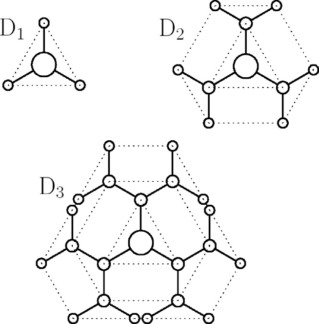
During the past decade dendritic molecular systems or dendrimers have received considerable attention Tomalia90 ; Frechet94 ; Mukamel97 ; Jiang97 ; Vogte98 ; Frechet01 . Dendrimers are synthetic highly branched tree-like macromolecules consisting of a core and several branches which are not connected geometrically to each other and are built self-similarly. Theoretically the process of building a dendrimer can be repeated ad infinitum to obtain a dendrimer with any number of generations, but in practice this number is currently limited to fifteen Frechet01 . The first three dendrimers with coordination number $z=3$ are schematically depicted in Fig. 1.

Dendrimers hold great promise for creating artificial light harvesting systems. Indeed, because of their branched nature, the number of units at their periphery grows exponentially with the number of generations . Therefore, if light absorbing states are located at the periphery, the cross-section of absorption grows exponentially with the number of generations. Combining this with a possibly efficient energy transport to the core may result in efficient light harvesting systems Frechet94 ; Mukamel97 ; Jiang97 .

A growing flux of publications exists, both experimental Devadoss96 ; Kopelman97 ; Jiang98 ; Hofkens99 ; Yeow00 ; Varnavski00 ; Andronov00 ; Drobizhev00 ; Texier01 ; Kleiman01 ; Varnavski02 and theoretical Barhaim97 ; Barhaim98 ; Rana03 ; Tretiak98 ; Raychaudhuri00 ; Argyrakis00 ; Poliakov99 ; Bentz03 ; Nakano00 ; Kirkwood01 ; Reineker01 ; Nakano01 , reporting on optical and transport properties of dendritic systems. For instance, in Ref. Kopelman97, compact and extended polyphenylacetylene dendrimers in solution were studied experimentally. Interpreting their spectroscopic measurements, the authors argued that the optical excitations in these systems are localized on dendrimer subunits. They also made the important point that extended dendrimers were characterized by a so-called energy funnel: the excitation energies of dendrimer units decreases from the periphery towards the core, thus providing an energetic bias for transport of the excitation towards the core. Such a bias is favorable for efficient transport of the absorbed energy across the dendrimer. Using quantum chemical calculations, the existence of an energy funnel towards the core was further confirmed in Ref. Tretiak98, . Experimental investigations of the energy transport in these systems Devadoss96 revealed the fact that it occurred through a multi-step (incoherent) hopping process with an efficiency of 96%. On the other hand, low-temperature measurements of the energy transport in distyrylbenzene-stilbene dendrimers with a nitrogen core gave clear indications of coherent interactions between the dendrimer subunits Varnavski02 . In this class of organic dendrimers, ultra-fast higher-order nonlinearities were also reported Varnavski00 , which makes them potentially promising systems for applications in nonlinear optical switching elements.

The first theoretical efforts on dendrimers were mostly focused on analyzing the mean first passage time, i.e., the average time it takes for an excitation, created somewhere at the periphery of the dendrimer, to reach its center, where a trap is located. This problem was addressed in much detail in Refs. Barhaim97 ; Barhaim98 ; Rana03 , where the mean first passage time was calculated both in the presence and the absence of a fixed energy bias. The presence of a random bias was considered in Ref. Raychaudhuri00 , where it was found that the randomness tends to reduce the transport efficiency. Large-scale numerical calculations of the statistics of the number of sites visited by the excitation and its mean square displacement in very large dendritic structures were performed in Ref. Argyrakis00 , while the authors of Ref. Bentz03 discussed the kinetics of symmetric random walks in compact and extended dendrimers of a small number of generations ($\leq 4$).

In all papers cited above, the basis of the analysis was the assumption of incoherent hopping transport between dendrimer units. However, the actual nature of the excitation transport and optical dynamics is still under debate. Thus, the alternative approach of coherent excitons extending over several dendrimer units has also been considered, in particular to describe energy transport from the periphery to the core Poliakov99 ; Nakano00 ; Kirkwood01 ; Reineker01 and the enhancement of the third-order optical susceptibility Nakano01 . An other interesting branch of experimental and theoretical studies of dendritic systems concerns the dynamics of dendrimer-based networks, i.e., extended systems using dendrimers as building blocks Jahromi01 ; Gitsov02 ; Dvornic02 ; Gurtovenko03 . Recently, such networks have attracted much attention due to their two levels of structural organization.

Among the factors that govern the efficiency of energy transport in dendritic systems, such as the energy bias and the presence of disorder, the radiative and non-radiative decay of optical excitations during their random walk to the core represents an additional channel, especially for dendrimers with a large number of generations. To the best of our knowledge, this factor has thus far not been addressed in the literature. Moreover, the statistics of the trapping time has not been studied in detail either. In this paper, we intend to fill these gaps and show that intimate relations exist between the analysis of both issues. We will show that in the presence of decay, the key parameter that governs the trapping efficiency is the product of the on-site excitation decay rate and the mean first passage time in the absence of decay.

The outline of this paper is as follows. In Section II we present our model, which is based on incoherent motion of excitations across the dendrimer, described by a rate equation that accounts for both trapping at the core and excitation decay during the random walk towards the core. We also discuss several quantities relevant to the problem under study, such as the distribution of survival times, the mean survival time, and the efficiency of trapping. Section III deals with deriving exact expressions for these quantities in the Laplace domain. In Sec. IV, we present a detailed analysis of the trapping time distribution in the limit of vanishing excitation decay. Effects of the excitation decay on the trapping efficiency under various conditions (sign of the energy bias, number of generations, ratio of decay and hopping rates) are discussed in Sec. V. Finally, we conclude in Sec.  VI.

II Model and pertinent quantities

As was already mentioned in the Introduction, we treat both the motion of the excitation over the dendrimer units and the trapping at the core as incoherent nearest-neighbor hopping processes. We label the dendrimer units (sites) by the index $i$ ($1\leq i\leq\cal{N}$), where $\cal{N}$ is the number of units, while $i=0$ denotes the trap located at the core (cf. Fig. 1). The trap is considered irreversible, i.e., once the excitation hops onto it, it never returns to the body of dendrimer. Then, the system of rate equations for the excitation probabilities (populations) $p_{i}$ of the dendrimer units reads

$${\dot{p}}_{0}=\sum_{\{j\}}k_{0j}p_{j}\ ,$$ (1a)

$${\dot{p}}_{i}=-\gamma p_{i}-\sum_{\{j\}}k_{ji}p_{i}+{\sum_{\{j\}}}^{\prime}k_{ij}p_{j}\ \quad(i\neq 0).$$ (1b)

Here, the dot denotes the time derivative, the summation $\sum_{\{j\}}$ is performed over sites $j$ that are nearest-neighbors of the site $i$, the prime in the second summation of Eq. (1b) indicates that $j\neq 0$, $\gamma$ is the exciton decay rate (assumed independent of $i$), and $k_{ij}$ is the rate of hopping from site $j$ to site $i$, including $i=0$. The hopping rates meet the principle of detailed balance: $k_{ij}=k_{ji}\exp[(E_{j}-E_{i})/k_{B}T]$, where $E_{i}$ is the excitation energy of the site $i$, $k_{B}$ is the Boltzmann constant, and $T$ is the temperature. In this sense the energy of the trap, $E_{0}$, is considered infinitely low. Initially, the excitation is outside the trap, i.e., $p_{0}(0)=0$, while one of dendrimer units is excited, $p_{i}(0)=\delta_{ii_{0}}$.

The quantity $r(t)\equiv{\dot{p}}_{0}$ represents the instantaneous trapping rate and will be used to study the time-domain behavior of the energy transport in dendritic systems. It can be expressed through the total population outside the trap, $\psi={\sum}^{\prime}_{i}p_{i}$, which is hereafter referred to as the survival probability with respect to both decay and trapping. Indeed, from Eqs. (1) it follows that $\sum_{i}{\dot{p}}_{i}\equiv{\dot{p}}_{0}+{\dot{\psi}}=-\gamma\psi$, so that for $r(t)$ one finds

$$r(t)=-\gamma\psi-{\dot{\psi}}\ .$$ (2)

Furthermore, the time dependence of $r(t)$ deriving from the decay constant $\gamma$, can be extracted explicitly by the transformation $p_{i}=e^{-\gamma t}\tilde{p}_{i}$. After this transformation Eq. (2) is reduced to

$$r(t)=-e^{-\gamma t}{\dot{\Psi}}\equiv e^{-\gamma t}R(t)\ ,$$ (3)

where $\Psi(t)={\sum}^{\prime}_{i}\tilde{p}_{i}$, and the $\tilde{p}_{i}$ now obey Eq. (1b) with $\gamma=0$. Thus, $\Psi$ is the analog of $\psi(t)$ and represents the total population outside the trap in the absence of excitation decay. It is the survival probability with respect to trapping alone. We see from Eq. (3) that in the time domain, the trapping and the decay of the excitations are independent of each other. Therefore, the time behavior of the trapping process can be studied separately, which simplifies the analysis.

The quantity $R(t)\equiv-{\dot{\Psi}}$ is normalized to unity for finite systems (in sense that $\int_{0}^{\infty}R(t)dt=1$) and represents the probability distribution of the (pure) trapping time. From this, the mean trapping time, often referred to as the mean first passage time Barhaim97 , is calculated in a standard way

$$\langle t\rangle=\int_{0}^{\infty}tR(t)\,{\rm d}t=\int_{0}^{\infty}\Psi(t)\,{\rm d}t\ .$$ (4)

The inverse quantity $\langle t\rangle^{-1}$ represents the effective trapping rate in the absence of excitation decay. Note that Eq. (4) can be rewritten via the Laplace transform $\tilde{R}(s)=\int_{0}^{\infty}e^{-st}R(t)\,{\rm d}t$ of $R(t)$:

$$\langle t\rangle=-\frac{{\rm d}\tilde{R}}{{\rm d}s}\Big{|}_{s=0}\ ,$$ (5)

which is useful for further considerations (see below).

We now define the efficiency of trapping (denoted as $\varepsilon$) as the total population that is transferred to the trap, i.e., the fraction of the initially created excitation that reaches the trap during its lifetime:

$$\varepsilon\equiv\lim_{t\rightarrow\infty}p_{0}(t)=\int_{0}^{\infty}r(t)\,{\rm d}t=\int_{0}^{\infty}e^{-\gamma t}R(t)\,{\rm d}t=\tilde{R}(s)|_{s=\gamma}\ .$$ (6)

An other important quantity that contains information about the trapping efficiency is

$$\tau=\int_{0}^{\infty}\psi(t)\,{\rm d}t=\frac{1-\varepsilon}{\gamma}\ ,$$ (7)

which is the mean survival time (with respect to both trapping and decay). Using this definition, we can, by convention, define the effective trapping rate $W$ in the presence of excitation decay as

$$W=\frac{1}{\tau}-\gamma=\frac{\varepsilon}{1-\varepsilon}\gamma\ ,$$ (8)

It should be stressed that $\varepsilon$, $\tau$, and $W$, being defined through time-integrations, are influenced by the excitation decay. In particular, if the latter occurs on a time scale much slower than the mean first passage time $\langle t\rangle$, the trapping efficiency $\varepsilon$ is close to unity, the survival time $\tau$ is reduced to the mean first passage time $\langle t\rangle$, given by Eq. (4), and $W\approx\langle t\rangle^{-1}$. If however the excitation decay occurs on a time scale that is comparable to or faster than the mean first passage time, the quantities $\varepsilon$, $\tau$, and $W$ will be determined by the interplay of the random walk to the trap and the excitation decay. This interplay between trapping and decay will be one of the main issues in the remainder of this paper.

To conclude this section we notice that all quantities relevant to the excitation energy transport, such as $\langle t\rangle$, $\varepsilon$, $\tau$, and $W$, are directly related to the Laplace transform $\tilde{R}(s)$ of the trapping time distribution $R(t)$ in the absence of decay. In the next section, we will provide the exact solution for $\tilde{R}(s)$.

III Laplace domain analysis: exact results

From now on, we will consider a specific model for the hopping process, in which only two different hopping rates occur. Specifically, we will assume that the hopping rates towards and away from the dendrimer’s core are, respectively, $k_{1}$ and $k_{2}$, no matter at which branching point of the dendrimer the excitation resides. This assumption corresponds to the situation with a linear energy bias, where the excitation energy difference between units of generation $M$ and $M-1$ is a constant, $\Delta E$, which is identical for every $M$. As was pointed out in Ref. Hughes82 , in this case the random walk across the dendrimer may be mapped onto a random walk on an asymmetric linear chain, where the rate of hopping is $k_{1}$ in the direction of one end of the chain (where the trap resides) and $(z-1)k_{2}$ in the other direction. In other words, instead of a dendrimer of generation $N$ a linear chain of length $N+1$ is considered with a trap at site $0$. This mapping is illustrated in Fig. 2.

After this mapping, the set of rate equations is different for dendrimers of one, two, and $N>2$ generations. For a one-generation dendrimer, only one equation occurs:

$$\dot{P}_{1}=-k_{1}P_{1}\ .$$ (9)

For a dendrimer with two or more generations, we have the following equations:

$$\dot{P}_{1}=-\left[k_{1}+(z-1)k_{2}\right]P_{1}+k_{1}P_{2}\ ,$$ (10a)

$$\dot{P}_{M}=(z-1)k_{2}P_{M-1}-\left[k_{1}+(z-1)k_{2}\right]P_{M}+k_{1}P_{M+1}\ ,\quad 1<M<N\ ,$$ (10b)

$$\dot{P}_{N}=(z-1)k_{2}P_{N-1}-k_{1}P_{N}\ ,$$ (10c)

where in case $N=2$, Eq. (10b) is absent. In all these equations, $P_{M}$ denotes the total population in the $M$th dendrimer generation, while the factor $z-1$ accounts for the number of nearest-neighbor units towards the periphery for each branching point. From this form it is clearly seen that the branching ($z\geq 2$) leads to a “geometrical” bias towards the dendrimer’s periphery, even in the absence of an energetic bias ($\Delta E=0$). Whether a net bias exists and in what direction, depends on the quantity $\kappa=(z-1)k_{2}/k_{1}=(z-1)\exp({-\Delta E}/k_{B}T)$. At $\kappa=1$ ($k_{1}=(z-1)k_{2}$), the geometrical and energetic biases exactly compensate each other, while for $\kappa<1$ ($\kappa>1$) a net bias towards (away) from the trap occurs.

As initial condition we will consider the situation where one excitation has been created at the periphery of the dendrimer, i.e., $P_{M}(0)=\delta_{MN}$. According to Eq. (1a), the trapping rate in the absence of excitation decay is now given by $R(t)=k_{1}P_{1}(t)$. This will be the quantity of our prime interest, for which we will seek a solution in the remainder of this section. Solving the one- and two-generation dendrimer problems is straightforward and will be done later on. Our main goal is to find the solution of the general problem of an $N$-generation dendrimer. This may be done in the Laplace domain. If for brevity we introduce the dimensionless time $t^{\prime}=k_{1}t$, Eqs. (10) written in the Laplace domain take the form:

$$0=-\left(1+\kappa+s\right)\tilde{P}_{1}+\tilde{P}_{2}\ ,$$ (11a)

$$0=\kappa\tilde{P}_{M-1}-\left(1+\kappa+s\right)\tilde{P}_{M}+\tilde{P}_{M+1},\ \quad 1<M<N\ ,$$ (11b)

$$-1=\kappa\tilde{P}_{N-1}-\left(1+s\right)\tilde{P}_{N}\ ,$$ (11c)

where the Laplace parameter $s$ is now in units of $k_{1}$ and $\tilde{R}=\tilde{P_{1}}$ (we use a tilde to denote the Laplace transformed functions). Below, we find a recursive relation for $\tilde{R}$, connecting this quantity for dendrimers of different numbers of generations (i.e., lengths of the effective linear chain). Therefore, we will from now on denote $\tilde{R}$ for a dendrimer of $N$ generations as $\tilde{R}_{N}$.

After $N-2$ steps of eliminating $\tilde{P}_{N},\tilde{P}_{N-1},...,\tilde{P}_{3}$ from Eqs. (11b) and (11c), we arrive at two coupled equations

$$0=-\left(1+\kappa+s\right)\tilde{P}_{1}+\tilde{P}_{2}\ ,$$ (12a)

$$-B_{N}=A_{N}\tilde{P}_{1}-\tilde{P}_{2}\ ,$$ (12b)

a solution of which with respect to $\tilde{P}_{1}=\tilde{R}_{N}$ is

$$\tilde{R}_{N}=\frac{B_{N}}{1+\kappa+s-A_{N}}\ .$$ (13)

Here, $A_{N}$ and $B_{N}$ are functions of the Laplace parameter $s$, which will be specified later on. For a dendrimer of $N+1$ generations, similarly, $N-2$ steps of excluding $\tilde{P}_{N+1},\tilde{P}_{N},...,\tilde{P}_{4}$ from Eqs. (11b) and (11c) yield a system of three coupled equations

$$0=-\left(1+\kappa+s\right)\tilde{P}_{1}+\tilde{P}_{2}\ ,$$ (14a)

$$0=\kappa\tilde{P}_{1}-\left(1+\kappa+s\right)\tilde{P}_{2}+\tilde{P}_{3}\ ,$$ (14b)

$$-B_{N}=A_{N}\tilde{P}_{2}-\tilde{P}_{3}\ ,$$ (14c)

where $A_{N}$ and $B_{N}$ are the same as in Eqs. (12a), (12b), and (13), while now $\tilde{P}_{1}=\tilde{R}_{N+1}$. Solving Eqs. (14a)-(14c) with respect to $\tilde{P}_{1}$ leads to an expression that is algebraically identical to Eq. (13), except that $A_{N}$ and $B_{N}$ are replaced by $A_{N+1}$ and $B_{N+1}$, respectively. The latter are given by

$$A_{N+1}=\frac{\kappa}{1+\kappa+s-A_{N}}\ ,$$ (15a)

$$B_{N+1}=\frac{B_{N}}{1+\kappa+s-A_{N}}\ ,$$ (15b)

and represent the recursive relations for these two functions. From comparison of Eq. (15) with Eq. (13), one finds that $B_{N+1}=\tilde{R}_{N}$ and $A_{N+1}=\kappa\tilde{R}_{N}/\tilde{R}_{N-1}$. Substituting these relations back into Eq. (13), we arrive at a recursive relation for $\tilde{R}_{N}$:

$$\frac{1}{\tilde{R}_{N}}=(1+\kappa+s)\frac{1}{\tilde{R}_{N-1}}-\kappa\frac{1}{\tilde{R}_{N-2}}\ .$$ (16)

Note that Eq. (16) can be used for $N>2$ only. In order to close the recursive iteration, $\tilde{R}_{1}$ and $\tilde{R}_{2}$ must be calculated separately. In the Laplace domain the solution of Eq. (9) for $N=1$ and Eqs. (10a) and (10c) for $N=2$ is straightforward and gives us the necessary quantities:

$$\tilde{R}_{1}=\frac{1}{1+s}\ ,$$ (17a)

$$\tilde{R}_{2}=\frac{1}{1+(2+\kappa)s+s^{2}}\ .$$ (17b)

Using Eqs. (17a) and (17b) in the recursive relation Eq. (16) and solving this relation, we finally obtain $\tilde{R}_{N}(s)$ in closed form:

$$\frac{2^{N+1}}{\tilde{R}_{N}} = \left(1+\frac{1-\kappa+s}{\sqrt{(1+\kappa+s)^{2}-4\kappa}}\right)\left(1+\kappa+s+\sqrt{(1+\kappa+s)^{2}-4\kappa}\right)^{N}$$ (18)

$$+ \left(1-\frac{1-\kappa+s}{\sqrt{(1+\kappa+s)^{2}-4\kappa}}\right)\left(1+\kappa+s-\sqrt{(1+\kappa+s)^{2}-4\kappa}\right)^{N}.$$

This is the principal result of this section.

It should be noticed that, despite the fact that Eq. (18) contains square roots, ${\tilde{R}_{N}}^{-1}$ in reality is a polynomial of $N$th order in $s$. This may be checked by explicit expansion of Eq. (18) in powers of $s$. Alternatively, the recursive relation Eq. (16) itself already represents a proof of this statement.

IV Trapping time distribution

It turns out to be impossible to perform the transformation back to the time domain for the general result Eq. (18), implying that we do not obtain an explicit expression for the trapping time distribution. However, the moments of this distribution and its asymptotic form at large $N$ do allow for an analytical treatment. In this section, we will address these two topics. We will also show that the asymptotic form may already be reached for rather small dendrimers, making these analytical expressions of practical use.

IV.1 Moments

To study the moments of the trapping time distribution, we make use of the following relation:

$$\langle t^{n}\rangle_{N}\equiv\int_{0}^{\infty}t^{n}R_{N}(t)\,{\rm d}t=(-1)^{n}\frac{{\rm d}^{n}\tilde{R}_{N}}{{\rm d}s^{n}}\Big{|}_{s=0}\ .$$ (19)

Furthermore, we recall that $1/\tilde{R}_{N}$ is a polynomial of $N$th order in $s$ (see the previous section), and thus can be written as

$$\frac{1}{\tilde{R}_{N}}=\sum_{m=0}^{N}a_{N}^{(m)}s^{m}\ ,\quad\quad a_{N}^{(m)}=\frac{1}{m!}\left(\frac{{\rm d}^{m}}{{\rm d}s^{m}}\frac{1}{\tilde{R}_{N}}\right)\Big{|}_{s=0}\ .$$ (20)

Substituting Eq. (20) into Eq. (16) and comparing coefficients related to the same power of $s$, we obtain a recursive relation for $a_{N}^{(m)}$

$$a_{N}^{(m)}=a_{N-1}^{(m-1)}+\left(1+\kappa\right)a_{N-1}^{(m)}-\kappa a_{N-2}^{(m)}\ ,$$ (21)

where it is implied that $a_{N}^{(m)}=0$ for $m>N$ and $m<0$. From Eqs. (17a) and (17b) it follows that for $N=1$ and $N=2$,

$$a_{1}^{(0)}=a_{1}^{(1)}=a_{2}^{(0)}=a_{2}^{(2)}=1\ ,\quad a_{2}^{(1)}=2+\kappa\ .$$ (22)

This allows us to start the recursive procedure for $a_{N}^{(m)}$.

The first important conclusion concerning the expansion coefficients, which follows from Eq. (21), is that $a_{N}^{(0)}=1$ for any $N$. This simply means that the zero’th moment of the trapping time distribution $\tilde{R}_{N}(0)=1$, i.e., the distribution is normalized. As a consequence of this fact, one can elucidate the physical meaning of the second coefficient of the expansion Eq. (20). It appears to be equal to the first moment of the distribution $R_{N}$, which is nothing but the mean trapping time $\langle t\rangle_{N}$:

$$a_{N}^{(1)}=\frac{\rm d}{{\rm d}s}\frac{1}{\tilde{R}_{N}}\Big{|}_{s=0}=-\left(\frac{1}{\tilde{R}_{N}^{2}}\frac{{\rm d}\tilde{R}_{N}}{{\rm d}s}\right)\Big{|}_{s=0}=\langle t\rangle_{N}\ .$$ (23)

Substituting this result in Eq. (21), yields a recursive formula for $\langle t\rangle_{N}$

$$\langle t\rangle_{N}=1+(1+\kappa)\langle t\rangle_{N-1}-\kappa\langle t\rangle_{N-2}\ ,$$ (24)

from which earlier results for the mean trapping time in dendrimers are reproduced Barhaim97 :

$$\langle t\rangle_{N}=\frac{1}{2}N(N+1)\ ,\quad\quad\quad\kappa=1\ ,$$ (25a)

$$\langle t\rangle_{N}=\frac{N}{1-\kappa}+\frac{\kappa}{(1-\kappa)^{2}}\left[\kappa^{N}-1\right]\ ,\quad\quad\kappa\neq 1\ .$$ (25b)

The next coefficient, $a_{N}^{(2)}$, contains information about the second moment of $R_{N}$. It is straightforward to show that

$$a_{N}^{(2)}=\langle t\rangle_{N}^{2}-\frac{1}{2}\langle t^{2}\rangle_{N}\ .$$ (26)

On the other hand, using Eq. (21) and the method of induction, one may show that

$$a_{N}^{(2)}=\frac{1}{24}(N-1)N(N+1)(N+2)\ ,\quad\quad\kappa=1\ ,$$ (27a)

$$a_{N}^{(2)} = \frac{\kappa^{N+1}[\kappa(N-1)-(N+2)]}{(1-\kappa)^{4}}$$ (27b)

$$+ \,\frac{N(N+1)}{2(1-\kappa)^{2}}+\,\frac{\kappa^{2}(N+1)+2\kappa-N}{(1-\kappa)^{4}}\ ,\quad\quad\quad\kappa\neq 1\ .$$

Making now use of Eqs. (25) and (27) in Eq. (26), we find $\langle t^{2}\rangle_{N}$:

$$\langle t^{2}\rangle_{N}=\frac{1}{12}N(N+1)[5N(N+1)+2]\ ,\quad\quad\kappa=1\ ,$$ (28a)

$$\langle t^{2}\rangle_{N} = \frac{N(N+1)}{(1-\kappa)^{2}}+\frac{(6N+2)\kappa^{N+1}}{(1-\kappa)^{3}}$$ (28b)

$$+ \frac{2\kappa}{(1-\kappa)^{4}}[\kappa^{2N+1}+\kappa^{N}-2]\ ,\quad\quad\kappa\neq 1\ .$$

It is worthwhile to consider the asymptotic behavior of the first and second moments of $R_{N}$ at large $N$, the case of our primary interest. They are given by

$$\langle t\rangle_{N}=\frac{N}{1-\kappa}\ ,\quad\langle t^{2}\rangle_{N}=\frac{N(N+1)}{(1-\kappa)^{2}}\ ,\quad\quad\kappa<1\ ,$$ (29a)

$$\langle t\rangle_{N}=\frac{1}{2}N^{2}\ ,\quad\langle t^{2}\rangle_{N}=\frac{5}{12}N^{4}\ ,\quad\quad\kappa=1\ ,$$ (29b)

$$\langle t\rangle_{N}=\frac{\kappa^{N+1}}{(\kappa-1)^{2}}\ ,\quad\langle t^{2}\rangle_{N}=\frac{2\kappa^{2(N+1)}}{(\kappa-1)^{4}}\ ,\quad\quad\kappa>1\ .$$ (29c)

These formulas already allow us to make a prediction concerning the shape of the trapping time distribution. In particular, comparing Eqs. (29b) and (29c) with Eq. (29a), we conclude that a drastic difference must exist between the two cases $\kappa<1$ (bias towards core) and $\kappa\geq 1$ (no bias or bias away from core), with respect to the shape of the trapping time distribution $R_{N}$. Indeed, calculating the standard deviation $\sigma_{N}=\sqrt{\langle t^{2}\rangle_{N}-\langle t\rangle_{N}^{2}}$, we obtain

$$\sigma_{N}=\frac{N^{1/2}}{1-\kappa}\ ,\quad\quad\kappa<1\ ,$$ (30a)

$$\sigma_{N}=\frac{N^{2}}{\sqrt{6}}\ ,\quad\quad\quad\kappa=1\ ,$$ (30b)

$$\sigma_{N}=\frac{\kappa^{N+1}}{(1-\kappa)^{2}}\ ,\quad\quad\kappa>1\ .$$ (30c)

As is seen, for large $N$, $\sigma_{N}\ll\langle t\rangle_{N}$ for $\kappa<1$, i.e., the distribution $R_{N}$ is narrow in the sense that its standard deviation is much smaller than its mean. By contrast, $\sigma_{N}\sim\langle t\rangle_{N}$ if $\kappa\geq 1$, which means that $R_{N}$ is a broad distribution in this sense.

IV.2 Asymptotic behavior, $N\gg 1$

From Eqs. (29) it follows that the characteristic time of trapping $\langle t\rangle_{N}$ in dendrimers of higher number of generation is long on the scale of the “effective” hopping times, which are $(1-\kappa)^{-1}$, $(\kappa-1)^{-1}$, and $2$ [or $(k_{1}-k_{2})^{-1}$, $(k_{2}-k_{1})^{-1}$, and $(2k_{1})^{-1}$ in dimensional units] for dendrimers with a total bias towards the trap ($\kappa<1$), towards the periphery ($\kappa>1$), and no bias ($\kappa=1$), respectively. Within the Laplace domain, this means that the dominant region of the parameter $s$, being of the order of $\langle t\rangle_{N}^{-1}$, is, respectively, small compared to $1-\kappa$, $\kappa-1$, and $2$ for these three different situations. This allows us to significantly simplify the expression Eq. (18) for $\tilde{R}_{N}$.

1. Total bias towards the trap, $\kappa<1$

We start analyzing the case of a total bias towards the trap ($\kappa<1$). Using a Taylor expansion of Eq. (18) with respect to $s/(1-\kappa)$, we obtain

$$\frac{1}{\tilde{R}_{N}}=\frac{s\kappa^{N+1}}{(1-\kappa)^{2}}\left(1-\frac{s}{1-\kappa}\right)^{N}+\left(1+\frac{s}{1-\kappa}\right)^{N}\ .$$ (31)

Since $\kappa<1$ and $N\gg 1$, the first term on the left-hand side can be neglected as compared to the second one, thus providing us with a very simple expression for $\tilde{R}_{N}$

$$\tilde{R}_{N}=\left(1+\frac{s}{1-\kappa}\right)^{-N}\ ,$$ (32)

which can be easily transformed back to the time domain. The result reads

$$R_{N}=\frac{(1-\kappa)^{N}}{(N-1)!}\>\>t^{N-1}\>\>e^{-(1-\kappa)t}\ .$$ (33)

We stress that this result is exact in the limit $\kappa\to 0$ (independent of $N$). As is seen, $R_{N}$ is strongly nonexponential and for $N\gg 1$ is characterized by a sharp profile, consistent with our findings in the previous subsection. In fact, in the limit of $s/(1-\kappa)\ll 1$ and $N\to\infty$ we can approximately write $\tilde{R}_{N}=\exp[-s\langle t\rangle_{N}]$, where $\langle t\rangle_{N}=N/(1-\kappa)$ is the mean trapping time for $\kappa<1$. The time-domain behavior, which corresponds to this Laplace transform, is $R_{N}=\delta(t-\langle t\rangle_{N})$. The nonexponentiality found is in fact a characteristic property of the trapping in dendrimers with a total bias towards the trap ($\kappa<1$), independent of the number of generations $N$.

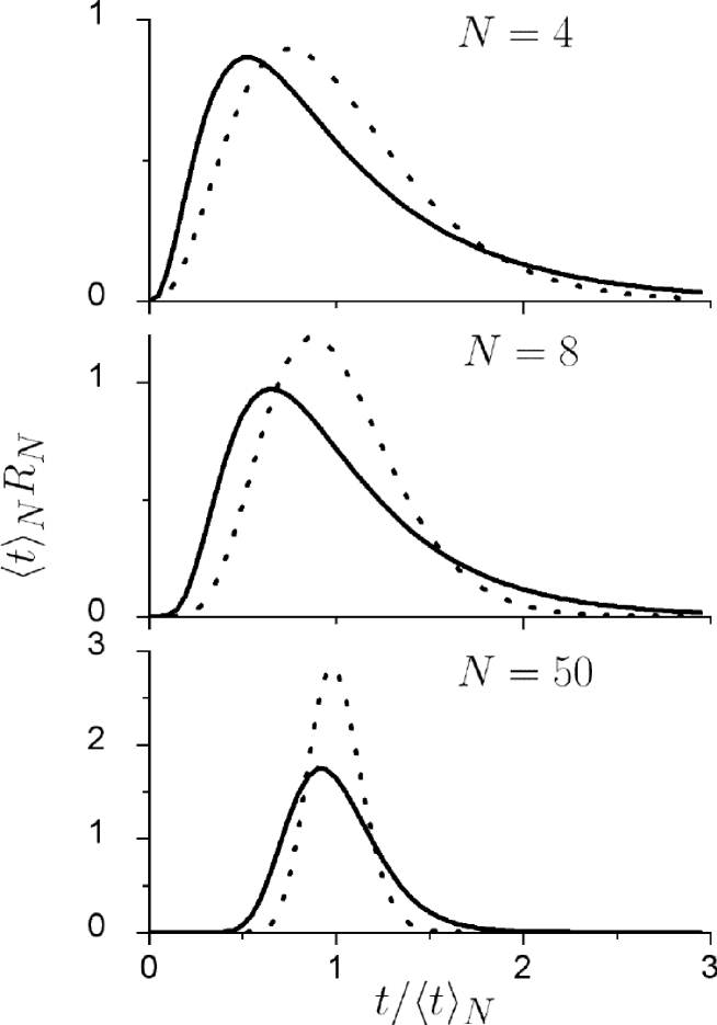
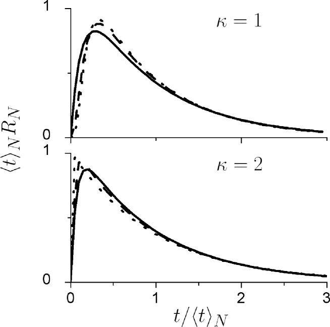
In order to illustrate how the approximate expression Eq. (33) fits the exact result obtained by numerically integrating Eqs. (10), we plotted in Figs. 3 and 4 the distribution $R_{N}$ calculated for $\kappa=1/5$ and $\kappa=1/2$ at different number of generations $N$. Here the solid lines are the exact solutions and the dashed lines correspond to the approximation Eq. (33). From these plots we conclude that for $\kappa=1/5$, Eq. (33) works well, even for dendrimers with only four generations. On the other hand, for $\kappa=1/2$ the deviation of Eq. (33) from the exact solution gets larger. These figures also clearly demonstrate the tendency of the trapping time distribution for large dendrimers to tend towards a delta-function at the mean-first passage time.

2. Zero total bias, $\kappa=1$

At zero total bias, i.e., when the energetic bias and geometrical one compensate each other ($\kappa=1$), the problem we are dealing with is equivalent with the classical one-dimensional diffusion problem on a finite segment with absorbing and reflecting boundary conditions at $x=0$ and $x=N$, respectively, and an initial condition corresponding to the creation of a diffusing object at $x=N$. The Laplace transform $\tilde{R}_{N}$, derived from Eq. (18) in the limit of $s\ll 2$, reads

$$\tilde{R}_{N}=\frac{1}{\big{(}1+\sqrt{s}\>\big{)}^{N}+\big{(}1-\sqrt{s}\>\big{)}^{N}}\approx\frac{2}{\cosh\big{(}\sqrt{2s\langle t\rangle_{N}}\>\big{)}}\ ,$$ (34)

where $\langle t\rangle_{N}=N^{2}/2$ is the mean trapping time in the diffusive regime of the random walk, and we used the fact that $(1\pm\sqrt{s})^{N}\approx e^{\pm N\sqrt{s}}$ for $s\ll 1$ and $N\gg 1$. In the time domain we then obtain

$$R_{N}=\frac{\pi}{\langle t\rangle_{N}}\sum_{n=0}^{\infty}(-1)^{n}\left(n+\frac{1}{2}\right)\>\>\exp\left[-\frac{\pi^{2}(n+1/2)^{2}t}{2\langle t\rangle_{N}}\right]\ .$$ (35)

In Fig. 5 (upper panel), we depicted $R_{N}(t)$ calculated by numertically integrating Eqs. (10) for dendrimers of different numbers of generations with $\kappa=1$. First, we note that the curves obtained for $N=4$ and $N=8$ are almost identical. Second, the dotted curve in the plot, corresponding to $N=8$, coincides in fact with the limiting curve; it is not changed by further increasing $N$. The decaying part of this curve is nicely fitted by the first term of the series Eq. (35), i.e., by $\exp(-\pi^{2}t/8\langle t\rangle_{N})$. Thus, we conclude that already for small $N$, the approximate result Eq. (35) gives a good fit to the exact result, and the tail of $R_{N}(t)$ is described by a single exponential.

3. Total bias towards the periphery, $\kappa>1$

We proceed similarly to the above in the case of a total bias towards the dendrimer periphery ($\kappa>1$). Assuming now in Eq. (18) that $s/(\kappa-1)\ll 1$, one finds

$$\frac{1}{\tilde{R}_{N}}=\frac{s\kappa^{N+1}}{(\kappa-1)^{2}}\left(1+\frac{s}{\kappa-1}\right)^{N}+\left(1-\frac{s}{\kappa-1}\right)^{N}\ .$$ (36)

We recognize here $\langle t\rangle_{N}=\kappa^{N+1}/(\kappa-1)^{2}$ as the mean trapping time for $\kappa>1$ [see Eq. (29c)]. As the relevant region of the Laplace parameter is determined by $s\langle t\rangle_{N}\sim 1$, while $\langle t\rangle_{N}\gg N/(k-1)$ at $\kappa>1$, the terms $s/(k-1)$ in the parentheses of Eq. (36) are negligible. Upon this simplification, $\tilde{R}_{N}$ takes the form

$$\tilde{R}_{N}=\frac{1}{s\langle t\rangle_{N}+1}\ ,$$ (37)

which, converted to the time domain, corresponds to the exponential behavior

$$R_{N}\approx\frac{1}{\langle t\rangle_{N}}\>\>\exp\left[-\frac{t}{\langle t\rangle_{N}}\right]\ .$$ (38)

Figure 5 (lower panel) illustrates this finding. All curves presented in this panel were obtained by numerically integrating Eqs. (10). As is seen, all curves are close to each other, including the one for $N=2$. The dotted curve is fitted very well by Eq. (38). From this we conclude that the approximation Eq. (38) works perfectly for any number of generations.

The difference in the behavior of $R_{N}$ (exponential or nonexponential) for different signs of the total bias in principle may be used to experimentally probe for the direction of the energetic bias in a dendrimer. Indeed, the kinetics of the fluorescence intensity $I(t)$ is proportional to $\psi=e^{-\gamma t}\left[1-\int_{0}^{t}R(t^{\prime})dt^{\prime}\right]$, i.e., is determined by two decay channels: the $\gamma$ processes and the trapping at the core. Having found the former from, for instance, the early-time decay of the intensity, we can then extract information about the direction of the energetic bias by measuring $I(t)$.

V Efficiency of trapping

In this section, we turn to analyzing the trapping efficiency $\varepsilon_{N}=\tilde{R}_{N}(s)|_{s=\gamma}$ (cf. Eq. 6), the exact expression for which follows directly from Eq. (18):

$$\frac{2^{N+1}}{\varepsilon_{N}} = \left(1+\frac{1-\kappa+\gamma}{\sqrt{(1+\kappa+\gamma)^{2}-4\kappa}}\right)\left(1+\kappa+\gamma+\sqrt{(1+\kappa+\gamma)^{2}-4\kappa}\right)^{N}$$ (39)

$$+ \left(1-\frac{1-\kappa+\gamma}{\sqrt{(1+\kappa+\gamma)^{2}-4\kappa}}\right)\left(1+\kappa+\gamma-\sqrt{(1+\kappa+\gamma)^{2}-4\kappa}\right)^{N}.$$

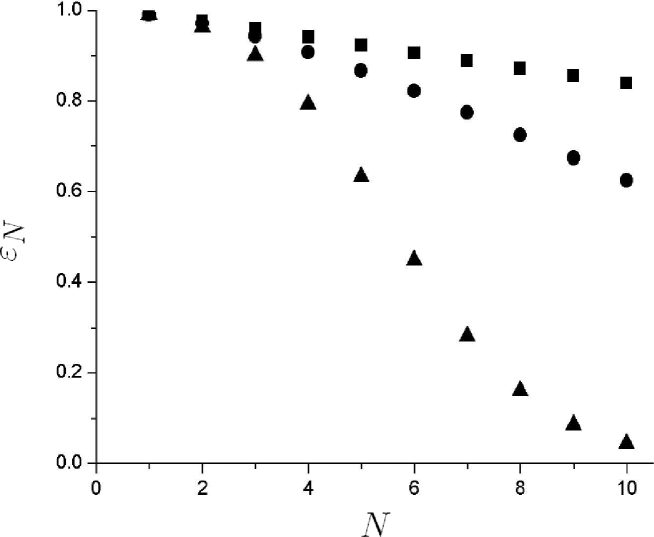
From this result, one easily generates plots for any set of variables $\kappa$, $\gamma$, and $N$. In particular, we present in Fig. 6 the results for the trapping efficiency according to Eq. (39), for dendrimers of $N=1$ to $N=10$ generations and different directions of the total bias, setting $\gamma=0.01$ (in units of $k_{1}$). The general trends displayed in this figure are easily understood. For small dendrimers, the efficiency is close to unity, unless a strong bias towards the periphery is combined with a fast decay. For larger dendrimers, the efficiency decreases due to an increased chance of decay before reaching the core. This effect grows when increasing the number of generations. However, a more detailed physical interpretation of Eq. (39) for larger $N$ values requires a deeper analysis. In the following, we will focus on this large-$N$ region. It is then natural to limit ourselves to a decay rate $\gamma$ that is small compared to the “effective hopping rates” $1-\kappa$, $\kappa-1$, and $2$, as we also assumed with respect to the Laplace parameter $s$ in our analysis of the trapping time distribution [see Sec. IV.2]. Otherwise, the trapping efficiency will be low even for a dendrimer of a small number of generations. Hereafter, we impose this condition, which allows us to directly use Eqs. (32), (34), and (37), replacing $s$ by $\gamma$.

1. Total bias towards the trap, $\kappa<1$

We first consider the case of a total bias towards the trap ($\kappa<1$). The corresponding expression for $\varepsilon_{N}$ is

$$\varepsilon_{N}=\left(1+\frac{\gamma}{1-\kappa}\right)^{-N}=\exp\left(-\frac{\gamma N}{1-\kappa}\right)=\exp\left[-\gamma\langle t\rangle_{N}\right]\ .$$ (40)

As is seen from this equation, the only parameter that determines the trapping is $\gamma\langle t\rangle_{N}=\gamma N/(1-\kappa)$. The interplay of trapping in the absence of excitation decay and the excitation decay itself determines the trapping efficiency: the latter is high (close to unity) for $\gamma\langle t\rangle_{N}\ll 1$, decreasing linearly with $\gamma\langle t\rangle_{N}$, and exponentially small in the opposite limit, $\gamma\langle t\rangle_{N}\gg 1$. We note that Eq. (40) implies that in the large-$N$ limit with $\kappa<1$, $\langle\exp[-\gamma t]\rangle=\exp[-\gamma\langle t\rangle]$, which is due to the fact that under these conditions the trapping time distribution tends to a delta function at the mean trapping time, as we have found in Sec. IV.2.

Using the definitions Eqs. (7) and (8), we can also calculate the mean survival time $\tau_{N}$ and the effective trapping rate $W_{N}$. They are given by

$$\tau_{N}=\frac{1}{\gamma}\Big{[}1-\exp\big{(}-\gamma\langle t\rangle_{N}\big{)}\Big{]}\ ,$$ (41a)

$$W_{N}=\frac{\gamma}{\exp\big{(}\gamma\langle t\rangle_{N}\big{)}-1}\ .$$ (41b)

If the decay is slow on the scale of the mean trapping time ($\gamma\langle t\rangle_{N}\ll 1$), the survival time $\tau_{N}$ coincides with the mean trapping time $\langle t\rangle_{N}$, and $W_{N}$ is just the inverse value $\langle t\rangle_{N}^{-1}$. In the opposite limit ($\gamma\langle t\rangle_{N}\gg 1$), we get $\tau_{N}=\gamma^{-1}$ (because the excitation cannot reach the trap within its lifetime) and $W_{N}=\gamma\exp[-\gamma\langle t\rangle_{N}]$. Note that the range of variation of $\tau_{N}$ is always from $\langle t\rangle_{N}$ to $\gamma^{-1}$ upon increasing the driving parameter $\gamma\langle t\rangle_{N}$ from zero to values large compared to unity. This is the general behavior of the survival time $\tau_{N}$, independent of the direction of the total bias.

2. Zero total bias, $\kappa=1$

In the diffusive regime ($\kappa=1$), according to Eq. (34),

$$\varepsilon_{N}=\frac{1}{\cosh\sqrt{2\gamma\langle t\rangle_{N}}}\ ,$$ (42)

and consequently

$$W_{N}=\frac{\gamma}{2\sinh^{2}\sqrt{\gamma\langle t\rangle_{N}/2}}\ ,$$ (43)

where now $\langle t\rangle_{N}=N^{2}/2$ is the trapping time for $\kappa=1$. In the limit of slow decay on the time scale of trapping ($\gamma\langle t\rangle_{N}\ll 1$) one obtains

$$\varepsilon_{N}=\frac{1}{1+\gamma\langle t\rangle_{N}}=\frac{1}{1+\gamma N^{2}/2}\ ,$$ (44)

i.e., the trapping efficiency is close to unity, as expected. In Eq. 44 we kept the “small” term in the denominator, because this expression works well even if $\gamma\langle t\rangle_{N}$ is slightly larger than unity. This is due to the fact that the Taylor expansion of the hyperbolic cosine only contains even powers of its argument.

If $\gamma\langle t\rangle_{N}$ gets larger than unity, another regime of trapping comes into play:

$$\varepsilon_{N}=2\exp{\Big{[}-\sqrt{2\gamma\langle t\rangle_{N}}\Big{]}}=\exp\big{(}-\sqrt{\gamma}N\big{)}\ .$$ (45)

As is seen, asymptotically $\varepsilon_{N}$ decreases exponentially, with an exponent proportional to $N$ (and not $N^{2}$). This thus resembles the behavior of trapping in the case of a large bias towards the trap (cf. Eq. (40). The pre-factor $\sqrt{\gamma}$ in Eq. (45), however, is larger than in the case of a bias towards to the trap ($\gamma$). This is not surprising, because in the diffusive regime, the excitation makes steps towards the periphery that slow down the process of reaching the trap, allowing for a larger effect of excitation decay before trapping may occur.

Finally, the effective trapping rate $W_{N}$ starts from the value $\langle t\rangle_{N}^{-1}$ in the limit of slow decay ($\gamma\langle t\rangle_{N}\ll 1$) and reveals the same behavior as $\varepsilon_{N}$ for $\gamma\langle t\rangle_{N}\gg 1$.

3. Total bias towards the periphery, $\kappa>1$

In a certain sense, this is the simplest case. For $s=\gamma$, Eq. (37) yields for the efficiency of trapping

$$\varepsilon_{N}=\frac{1}{1+\gamma\langle t\rangle_{N}}$$ (46)

for any ratio of $\langle t\rangle_{N}=\kappa^{N+1}/(\kappa-1)^{2}$ and $\gamma^{-1}$. Consequently, the relationship $W_{N}=\langle t\rangle_{N}^{-1}$ holds in general.

VI Conclusions

In this paper we theoretically studied the trapping of excitations in dendritic systems in the presence of (radiative and nonradiative) excitation decay when moving to the trap at the dendrimer’s center. We derived an exact expression for the Laplace transform of the trapping time distribution for a dendrimer of any number of generations. This expression was then used to analyze the general properties of pure trapping (in the absence of decay), focusing on dendrimers of a large number of generations. We found that the general nature of this distribution is governed by the total (geometrical and energetic) bias towards the trap. In the presence of a bias towards the trap, the trapping time distribution is narrow, in the sense that its standard deviation is small compared to its mean. The shape of the distribution is strongly nonexponential. Oppositely, in the presence of a bias towards the dendrimer’s periphery, the trapping time distribution is broad (its standard deviation is of the order of its mean), and its shape is essentially exponential with an exponent equal to the mean trapping time. The strong difference between both regimes is nicely illustrated by comparing Figs. 3 and 5. As the fluorescence kinetics is proportional to the trapping time distribution, the nature of the fluorescence decay (exponential or nonexponential) may in practice be used to distinguish the direction of the energetic bias in dendrimers. We also note that, although in the analysis of the trapping time distribution we used the limit of a large number of generations, it appears from comparison to numerically exact results that many of the analytical expressions hold even for small dendrimers, with just a few generations.

The trapping efficiency $\varepsilon$ was found to depend on the ratio of the decay time ($\gamma^{-1}$) and the trapping time in the absence of decay ($\langle t\rangle$). The product $x=\gamma\langle t\rangle$ turns out to be the only essential parameter that governs the trapping in the presence of excitation decay. For dendrimers with a total bias towards the trap ($\kappa<1$), the efficiency of trapping depends exponentially on this parameter within its entire range of values: $\varepsilon=e^{-x}$. In the diffusive regime of trapping, when the geometrical and energetic bias compensate each other ($\kappa=1$), $\varepsilon=1-x$ for $x<1$, while for $x>1$ this behavior changes to a stretched-exponential one, $\varepsilon\sim e^{-\sqrt{x}}$. For dendrimers with a total bias towards the periphery ($\kappa>1$), the trapping efficiency $\varepsilon=(1+x)^{-1}$, independent of $x$.

We finally notice that in practice the various regimes with regards to the total bias parameter $\kappa$ distinguished by us, may be probed experimentally in one and the same dendritic system by varying the temperature. In particular, $\kappa$ tends from zero at low temperature to $z-1$ at high temperature.

Figure 1: Schematic pictures of dendrimers of one (D₁), two (D₂), and three (D₃) generations with the coordination number $z=3$ (equal to the number of branches at each branching point). The large circle at the dendrimer center represents a trap, while the small circles are building units of the dendrimer branches, representing sites on which optical excitations can reside. Connected by the dotted lines are the dendrimer units belonging to the same generation.

Figure 2: Example of mapping of a dendrimer D₃ with $z=3$ and a linear energy bias onto an equivalent linear chain. The large circle represents the trap, while all units of generation $M(=1,2,3)$ are mapped onto one site $M$ of the linear chain, which is drawn by a small circle. The quantities $k_{1}$ and $k_{2}$ are the hopping rates towards and away from the trap, respectively, in the real dendrimer. The factor $z-1$ counts the number of branches towards the periphery at each branching point and multiplies $k_{2}$ to obtain the effective outward hopping rate in the equivalent linear chain.

Figure 3: Plots of the trapping time distribution $R_{N}(t)$ for dendrimers of different number of generations $N$ with a total bias towards the trap ($\kappa=1/5$). In all plots, the solid curves represent the exact solution for $R_{N}(t)$ obtained from numerically solving Eqs. (10), while the dashed curves correspond to the approximate expression Eq. (33).

Figure 4: Same as in Fig. 3, using $\kappa=1/2$.

Figure 5: Plots of the trapping time distribution $R_{N}(t)$ for dendrimers of different number of generations $N$ in the diffusive regime of hopping ($\kappa=1$) and for a total bias towards the periphery ($\kappa=2$). All curves were obtained by numerically solving Eqs. (10). In both panels, the solid curves correspond to $N=2$, the dashed curves to $N=4$, and the dotted curves to $N=8$. The decaying part of the latter curve in the upper panel coincides with $\exp[-\pi^{2}t/8\langle t\rangle_{N}]$.

Figure 6: Plots of the trapping efficiency $\varepsilon_{N}$ as a function of number of generations $N$ calculated for $\gamma=0.01$ and different values for $\kappa$. The squares correspond to $\kappa=1/2$ (total bias towards the trap), circles correspond to $\kappa=1$ (no total bias, diffusive regime of hopping), and the triangles correspond to $\kappa=2$ (total bias towards the periphery).

References

- (1) D. A. Tomalia, A. M. Naylor, and W. A. Goddard, Angew. Chem. Int. Ed. 29, 138 (1990).
- (2) J. M. J. Fréchet, Science 263, 1710 (1994).
- (3) S. Mukamel, Nature 388, 425 (1997).
- (4) D.-L. Jiang and T. Aida, Nature 388, 454 (1997).
- (5) F. Vögte , ed., Dendrimers (Springer-Verlag, Berlin, 1998).
- (6) J. M. J. Fréchet and D. A. Tomalia, eds., Dendrimers and Other Dendric Polymers (John Wiley&Sons West Sussex, 2001).
- (7) C. Devadoss, P. Bharathi, J. S. Moore, J. Am. Chem. Soc. 118, 9635 (1996); M. Shortreed, S. F. Swallen, Z.-I. Shi, W. Tan, Z. Xu, C. Devadoss, J. S. Moore, and R. Kopelman, J. Phys. Chem. B 101, 6318 (1997).
- (8) R. Kopelman, M. Shortreed, Z.-I. Shi, W. Tan, Z. Xu, J. C. Moor, A. Bar-Haim, and J. Klafter, Phys. Rev. Lett. 78, 1239 (1997).
- (9) D.-L. Jiang and T. Aida, J. Am. Chem. Soc. 120, 10895 (1998); M. Kawa and J. M. J. Fréchet, Thin Solid Films 331, 259 (1998); D. ben-Avraham, L. S. Shulman, S. H. Bossmann, C. Turro, and N. J. Turro, J. Phys. Chem. B 102, 5088 (1998); M. I. Slush, I. G. Scheblykin, O. P. Varnavsky, A. G. Vitukhnovsky, V. G. Krasovskii, O. B. Gorbatsevich, and A. M. Muzafarov, J. Lumin. 76&77, 246 (1998).
- (10) J. Hofkens, L. Latterini, G. De Belder, T. Gensch, M. Maus, T. Vosch, Y. Karni, G. Schweitzer, F. C. De schryver, A. Hermann, and K. Müllen, Chem. Phys. Lett. 304, 1 (1999); M. Lor, R. De, S. Jordens, G. De Belder, G. Schweitzer, M. Gotlet, J. Hofkens, T. Weil, A. Herrmann, K. Múllen, M. Van Der Auweraer, and F. C. De Schryver, J. Phys. Chem. A 106, 2083 (2002).
- (11) E. K. L. Yeow, K. P. Ghiggino, J. N. H. Reek, M. J. Crossley, A. W. Bosman, A. P. H. J. Schenning, and E. W. Meijer, J. Phys. Chem. B 104, 2596 (2000).
- (12) O. Varnavski, A. Leanov, L. Lui, J. Takacs, and T. Goodson, III, J. Phys. Chem. B 104, 179 (2000); Phys. Rev. B 61, 12732 (2000); O. Varnavski, G. Menkir, and T. Goodson, III, Appl. Phys. Lett. 77, 1120 (2000); O. Varnavski, R. G. Ispasoiu, L. Balogh, D. A. Tomalia, and T. Goodson, III, J. Chem. Phys. 114, 1962 (2001).
- (13) A. Andronov, S. L. Gilat, J. M. J. Fréchet, K. Ohta, F. V. R. Neuwhal, and G. R. Flemming, J. Am. Chem. Soc. 122, 1175 (2000).
- (14) M. Drobizhev, A. Rebane, C. Sigel, E. H. Elandaloussi, and C. W. Spangler, Chem. Phys. Lett. 325, 375 (2000).
- (15) I. Texier, M. N. Berberan-Santos, A. Fedorov, M. Brettriech, H. Schönberger, A. Hirsch, S. Leach, and R. Bensasson, J. Phys. Chem. A 105, 10278 (2001).
- (16) V. D. Kleiman, J. S. Melinger, and D. McMorrow, J. Phys. Chem. B 105, 5595 (2001).
- (17) O. Varnavski, I. D. W. Samuel, L.-O. Palsson, R. Beavington, P. L. Burn, and T. Goodson, III, J. Chem. Phys. 116, 8893 (2002); O. P. Varnavski, J. C. Ostrowski, L. Sukhomlinova, R. T. Twieg, G. C. Bazan, and T. Goodson, III, J. Am. Chem. Soc. 124, 1736 (2002); M. I. Ranasinghe, O. P. Varnavski, J. Pawlas, S. I. Hauck, J. Louie, J. F. Hartwig, and T. Goodson, III, J. Am. Chem. Soc. 124, 6520 (2002); M. I. Ranasinghe, Y. Wang, and T. Goodson, III, J. Am. Chem. Soc. 125, 5258 (2003).
- (18) A. Bar-Haim, J. Klafter, and R. Kopelman, J. Am. Chem. Soc. 119, 6197 (1997).
- (19) A. Bar-Haim and J. Klafter, J. Lumin. 76&77, 197 (1998); J. Phys. Chem. B 102, 1662 (1998); J. Chem. Phys. 109, 5187 (1998).
- (20) D. Rana and G. Gangopadhyay, J. Chem. Phys. 118, 434 (2003).
- (21) S. Tretiak, V. Chernyak, and S. Mukamel, J. Phys. Chem. B 102, 3310 (1998);
- (22) S. Raychaudhuri, Y. Shapir, V. Chernyak, and S. Mukamel, Phys. Rev. Lett. 85, 282 (2000); S. Raychaudhuri, Y. Shapir, and S. Mukamel, Phys. Rev. E 65, 21803 (2002).
- (23) P. Argyrakis and R. Kopelman, Chem. Phys. 261, 391 (2000); D. Katsoulis, P. Argyrakis, A. Pimenov, and A. Vitukhnovskii, Chem. Phys. 275, 261 (2002).
- (24) J. L. Bentz, F. N. Hosseini, J. J. Kozak, Chem. Phys. Lett. 370, 319 (2003).
- (25) E. Poliakov, V. Chernyak, S. Tretiak, and S. Mukamel, J. Chem. Phys. 110, 8161 (1999).
- (26) M. Nakano, M. Takahata, H. Fujita, S. Kiribayashi, and K. Yamaguchi, Chem. Phys. Lett. 323, 249 (2000); M. Takahata, M. Nakano, H. Fujita, and K. Yamaguchi, Chem. Phys. Lett. 363, 422 (2002).
- (27) J. C. Kirkwood, C. Scheurer, V. Chernyak, and S. Mukamel, J. Chem. Phys. 114, 2419 (2001).
- (28) P. Reineker, A. Engelmann, and V. I. Yudson, J. Lumin. 94-95, 203 (2001).
- (29) M. Nakano, H. Fujita, M. Takahata, S. Kiribayashi, and K. Yamaguchi, Int. J. Quant. Chem. 84, 649 (2001).
- (30) S. Jahromi, V. Litvinov, and B. Coussens, Macromolecules 34, 1013 (2001).
- (31) I. Gitsov and C. Zhu, Macromomlecules 35, 8418 (2002).
- (32) P. R. Dvornic, J. Li, A. M. de Leuze-Jallouli, S. D. Reeves, and M. J. Owen, Macromomlecules 35, 9323 (2002).
- (33) A. A. Gurtovenko, D. A. Markelov, Yu. Ya. Gotlib, and A. Blumen, J. Chem. Phys. 119, 7579 (2003).
- (34) B. D. Hughes and M. Sahimi, J. Stat. Phys. 29, 781 (1982).