Generalized minority games with adaptive trend-followers and contrarians

Abstract

We introduce a simple extension of the minority game in which the market rewards contrarian (resp. trend-following) strategies when it is far from (resp. close to) efficiency. The model displays a smooth crossover from a regime where contrarians dominate to one where trend-followers dominate. In the intermediate phase, the stationary state is characterized by non-Gaussian features as well as by the formation of sustained trends and bubbles.

Financial markets are known to generate non-trivial fluctuation phenomena MS ; BP that are qualitatively reproduced by several models where agents with prescribed trading rules interact through a complex mechanism of price formation SantaFe ; Flo ; JDF ; LM99 ; GB03 . Originally devised to get a more fundamental grasp on the critical behavior of systems of heterogeneous agents, the minority game CZ was able to capture some of the complex macroscopic phenomenology of markets starting from primitive microscopic ingredients CMZ ; Hui ; CM03 , clarifying the roles of different factors contributing to the complexity of market dynamics. Still, many important issues escape a more basic investigation.

One of these is the interaction of different types of agents. Broadly speaking, traders can be divided in two groups, namely contrarians (or fundamentalists) and trend-followers (or chartists). The former believe that the market is close to a stationary state and buy (sell) when they repute the stock to be underpriced (overpriced), thus inducing anti-correlation in market returns and holding the price close to its ‘fundamental’ value. The latter, instead, extrapolate trends from recent price increments and buy or sell assuming that the next increment will occur in the direction of the trend, thus creating positive return correlations and large price drifts (‘bubbles’). Chartist behavior, which can also be driven by imitation, is known to cause market instability LM99 ; M01 . Fundamentalists act instead as a restoring force that dumps market inefficiencies and excess volatility. It has been argued M01 ; MHet that contrarians (trend followers) are described by minority (majority) game players (but see also AS03 ; FM03 ), and the analysis of mixed majority-minority games has shown that the presence of trend followers can severely alter the market’s efficiency DGM03 . However, agents in these models are committed to either one of the types, and switching from one group to the other, a key feature in other models LM99 , is not allowed.

Here we introduce a class of market games that bypasses this limitation. We assume that trend-following behavior dominates when price movements are small, as agents try to anticipate trends, whereas traders turn to a contrarian conduct when the market becomes chaotic. This mechanism causes a ‘feedback’ in the dynamics of the excess demand: when it is small, trend-followers dominate and drive it to larger values; but once it has become sufficiently large, contrarians take over and drive it back to smaller values by inducing anti-correlations. In this way, it is the market that determines whether trend-following or contrarian strategies gain and there is no need to employ different payoff functions. We will use the cutoff between the majority- (where trend-followers win) and the minority-regime (where contrarians win) as a control parameter to discriminate fundamentalists- and chartists-dominated phases. The most remarkable phenomenology occurs, not surprisingly, in-between the two.

Hereafter, we shall use the prefixes $<$- and $>$- for ‘minority’ and ‘majority’, respectively.

Our basic setup is as follows. At each time step $t$, $N$ agents receive an information $\mu(t)$ chosen at random from $\{1,\ldots,P\}$ with uniform probability. Based on $\mu(t)$, agents have to formulate a binary bid $b_{i}(t)$ (‘buy/sell’). To this aim, each of them is endowed with $S$ strategies $\boldsymbol{a}_{ig}=\{a_{ig}^{\mu}\}$ ($g=1,\ldots,S$) that map informations $\mu\in\{1,\ldots,P\}$ into actions $a_{ig}^{\mu}\in\{-1,1\}$. Each component $a_{ig}^{\mu}$ of every strategy is selected randomly and independently from $\{-1,1\}$ with equal probability for every $i$, $g$ and $\mu$ at the beginning of the game and fixed, so that strategies play the role of a quenched disorder. Finally, each strategy of every agent is given an initial valuation $p_{ig}(0)$ that is updated at the end of every round.

At each time step, every agent picks the strategy $\widetilde{g}_{i}(t)={\rm argmax}_{g}~{}p_{i,g}(t)$ with the largest valuation and formulates the bid $b_{i}(t)=a_{i\widetilde{g}_{i}(t)}^{\mu(t)}$. The (normalized) excess demand at time $t$, namely the mismatch between the total demand and the total supply, is defined as $A(t)=N^{-1/2}\sum_{i=1}^{N}b_{i}(t)$, and strategy valuations are updated according to

$$p_{ig}(t+1)=p_{ig}(t)+a_{ig}^{\mu(t)}F[A(t)]$$ (1)

where $F$ is a function embodying the rules with which payoffs are assigned or the way agent $i$ assesses the performance of his/her $g^{\rm th}$ strategy (in which case one could also assume that $F$ depends on $i$). In the $<$-game, $F(A)=-A$, so at each time step strategies suggesting the minority action are rewarded. In the $>$-game, instead, $F(A)=A$. Here we set

$$F(A)=A-\epsilon A^{3}$$ (2)

with $\epsilon\geq 0$. For $\epsilon=0$ one has a pure $>$-Game. Upon increasing $\epsilon$, the non-linear, $<$-term gains importance, and for $\epsilon\to\infty$ one obtains a $<$-game with $F(A)\propto-A^{3}$.

We want to characterize the steady state of (1) in the limit $N\to\infty$, as a function of the relative number of information patterns $\alpha=P/N<\infty$. In our experiments, we set $p_{ig}(0)=0$ for all $i$ and $g$, and $S=2$, and focused for a start on the observables $\sigma^{2}=\left\langle{A^{2}}\right\rangle$ and $H=\overline{\left\langle{A|\mu}\right\rangle^{2}}$, where $\left\langle{\cdots}\right\rangle$ and $\left\langle{\cdots|\mu}\right\rangle$ denote time averages in the stationary state, the latter conditioned on the occurrence of the information pattern $\mu$, and the over-line stands for an average over $\mu$’s ($\overline{\cdots}=(1/P)\sum_{\mu=1}^{P}\cdots$). Averages over the distribution of the quenched disorder (the strategies) are also performed. As discussed at length in the early $<$-game literature MCZ , $\sigma^{2}$ measures the magnitude of market fluctuations (the ‘volatility’), while $H$ quantifies the ‘predictability’ of the game, i.e. the presence of exploitable information: when $H=0$, the winning action cannot be predicted on the basis of $\mu$. Notice that $\sigma^{2}=1$ when agents buy and sell at random.

Results for these quantities are reported in Fig. 1 and 2.

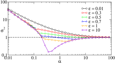
Figure 1: Volatility $\sigma^{2}$ as a function of $\alpha=P/N$ for different values of $\epsilon$. Simulations performed with $\alpha N^{2}=16000$, with averages over 100 disorder samples per point. A given sample corresponds to a particular realization of the strategies $\boldsymbol{a}_{ig}$.

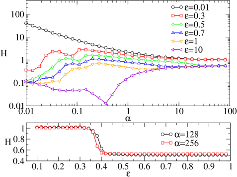
Figure 2: Predictability $H$ as a function of $\alpha=P/N$ for different values of $\epsilon$ (top) and the reverse (bottom). Simulation parameters are as in Fig. 1.

For small $\epsilon$, one recovers as expected a pure $>$-game, with $\sigma^{2}=H>1$ for all $\alpha$. As $\epsilon$ increases, the volatility displays a smooth change to a $<$-regime, with the onset of a cooperative phase where $\sigma^{2}$ is better-than-random. When $\epsilon\to\infty$, a minimum is formed close to the phase transition $\alpha_{c}\simeq 0.34$ of the standard $<$-game CMZ . The predictability $H$ shows a more articulated behavior. As $\epsilon$ increases, $H$ becomes smaller than $1$ at low $\alpha$ (as in a $<$-game), but it still tends to $1$ for large $\alpha$ (as in a $>$-game). Unfortunately, the low-$\alpha$ behavior is hard to characterize numerically as a function of $\epsilon$ since reliable experiments at $\alpha\leq 0.01$ require unrealistic CPU times. For high-$\alpha$, one can instead identify a sharp transition:

$$\lim_{\alpha\to\infty}H=\begin{cases}1&\text{for $\epsilon<\epsilon_{c}\simeq 0.37$}\\ 1/2&\text{for $\epsilon>\epsilon_{c}$}\end{cases}$$ (3)

A further increase of $\epsilon$ causes a reduction of exploitable information. However, no unpredictable regime with $H=0$ is detected at low $\alpha$ when $\epsilon\to\infty$, at odds with the standard $<$-game.

Another significant macroscopic observable is the fraction $\phi$ of “frozen” agents, that is, of players for which the difference $p_{i1}(t)-p_{i2}(t)$ between the strategy valuations diverges in the limit $t\to\infty$, so that they end up using only one of their strategies. The behavior of $\phi$ is shown in Fig. 3.

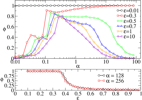
Figure 3: Fraction of frozen agents $\phi$ as a function of $\alpha=P/N$ for different values of $\epsilon$ (top) and the reverse (bottom). Simulation parameters are as in Fig. 1.

Again, for large $\alpha$ a sharp threshold separating a $>$-like regime with all agents frozen ($\epsilon<\epsilon_{c}$) from a $<$-like regime where $\phi=0$ ($\epsilon>\epsilon_{c}$) is found. For large $\epsilon$, $\phi$ has $<$-game’s characteristic shark-fin shape. Notice that as $\epsilon$ increases $\phi$ decreases, signaling that it becomes harder and harder for traders to identify an optimal strategy when the market is dominated by speculators. In the low-$\alpha$, large-$\epsilon$ phase, our agents are significantly more likely to be frozen than in a pure $<$-game. This feature, together with the absence of an unpredictable phase in the same conditions, is due to the non-standard nature of the $<$-regime in our model unpu .

The fact that $<$-like and $>$-like features can coexist at intermediate $\epsilon$ can be seen clearly by studying the correlation M01 ; FM03

$$D=\frac{\left\langle{A(t)A(t+1)}\right\rangle}{\left\langle{A(t)^{2}}\right\rangle}=\frac{\left\langle{A(t)A(t+1)}\right\rangle}{\sigma^{2}}$$ (4)

(see Fig. 4).

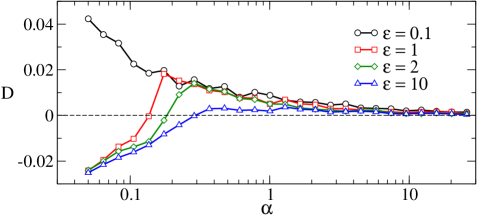
Figure 4: Normalized correlation function $D$ as a function of $\alpha=P/N$ for different values of $\epsilon$. Simulation parameters are as in Fig. 1.

For small $\epsilon$, $D$ is positive, signaling that the market dynamics is completely dominated by positive correlations (i.e. by trend-followers). As $\epsilon$ increases, anti-correlations appear at low $\alpha$. The contrarian phase becomes larger and larger as $\epsilon$ grows further and for $\epsilon\gg 1$ the market is dominated by contrarians.

We can shed some light on the crossover from the $<$- to the $>$-regime at large $\alpha$ for $S=2$ drawing inspiration from CM99 . Let us define, for each agent, the strategy valuation difference $y_{i}(t)=\frac{1}{2}[p_{i1}(t)-p_{i2}(t)]$, and note that the Ising spin $s_{i}(t)\equiv{\rm sign}[y_{i}(t)]$ determines the strategy that agent $i$ chooses at time $t$. It is simple to show that

$$v_{i}\equiv\left\langle{y_{i}(t+1)-y_{i}(t)}\right\rangle=\overline{\xi_{i}^{\mu}\left\langle{F(A)|\mu}\right\rangle}$$ (5)

where ${\xi}_{i}^{\mu}=\frac{1}{2}({a}_{i1}^{\mu}-{a}_{i2}^{\mu})$. If $v_{i}\neq 0$, then $y_{i}(t)\sim v_{i}t$ and $s_{i}(t)$ tends asymptotically to ${\rm sign}(v_{i})$: there is a well defined preference towards one of the two strategies and the agent becomes frozen. This is what happens for $\epsilon\ll 1$, i.e. in the $>$-game regime. Here, $A(t)$ is a function of $\mu(t)$ only (because all agents are frozen), therefore $\left\langle{A^{2}|\mu}\right\rangle=\left\langle{A|\mu}\right\rangle^{2}$ and $\sigma^{2}=H$. For large $\alpha$, when the agents’ strategic choices are roughly uncorrelated nota2 , we can approximate $A(t)$ with a Gaussian rv with variance $H$. By virtue of Wick’s theorem, this implies that $\left\langle{A^{3}|\mu}\right\rangle\simeq 3H\left\langle{A|\mu}\right\rangle$, so

$$v_{i}\simeq(1-3\epsilon H)\overline{\xi_{i}^{\mu}\left\langle{A|\mu}\right\rangle}$$ (6)

If $1-3\epsilon H>0$, the agents’ spins will freeze on the $>$-game solution $s_{i}={\rm sign}(\overline{\xi_{i}^{\mu}\left\langle{A|\mu}\right\rangle})$, which is unstable for $1-3\epsilon H\leq 0$. Given that $H=1$ for large $\alpha$, we see that the crossover from the $>$- to the $<$-regime takes place at $\epsilon\simeq 1/3$ for $\alpha\gg 1$. This estimate is significantly close to the numerical value of $\epsilon_{c}\simeq 0.37$. A similar argument can be run from the $<$-game side, where, at large $\alpha$, $A(t)$ can be approximated with a Gaussian random variable with variance $\sigma^{2}$ (in this case different from $H$), so that $\left\langle{A^{3}|\mu}\right\rangle\simeq 3\sigma^{2}\left\langle{A|\mu}\right\rangle$. Arguing as before, one finds that the stability condition of a $<$-game like solution is $1-3\epsilon\sigma^{2}<0$. Given that $\sigma^{2}=1$ for large $\alpha$, we find that the solution is $<$-game like for $\epsilon>1/3$ when $\alpha\gg 1$.

Unfortunately, the above argument is not valid at small $\alpha$ since $A(t)$ acquires strong non-Gaussian statistics, so the quality of the approximation gets worse and worse as $\alpha$ decreases. To see this, let us inspect the probability distribution $P(A)$ of $A(t)>0$ as a function of $\epsilon$ in the regimes of large and small $\alpha$ (see Fig. 5).

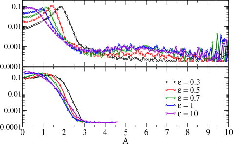
Figure 5: Probability distributions $P(A)$ of $A>0$ for different values of $\epsilon$ for $\alpha=0.05$ (top) and $\alpha=2$ (bottom). Simulation parameters are as in Fig. 1.

For $\alpha=2$ and $A$ not too large, one finds roughly that $\log P(A)\propto A^{2}-bA^{4}$ ($b=$constant) with a weak dependence on $\epsilon$. For $\alpha=0.05$, instead, $P(A)$ is considerably more sensitive to the the value of $\epsilon$ and cannot be fitted by a simple form as before. In this regime, where the contribution of frozen agents is small, we expect the system to self-organize around a value of $A$ such that $F(A)=0$: indeed one can see from Fig. 5 that the peak of the distribution moves as $1/\sqrt{\epsilon}$. Besides, as $\epsilon$ increases, large excess demands occur with a finite probability. The emergence of such ‘tails’ in $P(A)$, while not power-law, is a clear non-Gaussian signature.

In the light of these findings, it is interesting to inspect the typical market dynamics in the non-Gaussian regime. In Fig. 6 a single realization of the game at $\alpha=0.05$ and $\epsilon=1$ is displayed. In particular, we show the time series of excess returns and the time series of the price $R(t)=\sum_{t^{\prime}\leq t}A(t^{\prime})$ in the steady state. One can clearly see that while the market is mostly chaotic and dominated by contrarians, ‘ordered’ periods can arise where the excess demand is small and trends are formed, signaling that chartists have taken over the market. A detailed analysis clarifies that the spikes in $A(t)$ occur in coordination with the transmission of a particular information pattern $\nu$ to which the market responds by generating large excess demands. This phenomenon is reminiscent of the retrieval of stored patterns in neural networks, and was also found in $>$-games KM , although in the present case $A(t)$ is not of order $\sqrt{N}$. However, the ‘recalled’ pattern $\nu$ changes with time, and each pattern can be ‘active’ for many time steps in a row and then quiesce for just as long during a single run. These features make the dynamics strongly sample-dependent, in a way that is reminiscent of another recently studied variation of the $<$-game CMD .

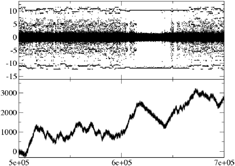
Figure 6: Single realization of market dynamics at $\alpha=0.05$ and $\epsilon=1$. Top: $A(t)$ vs $t$. Bottom: $R(t)$ vs $t$.

In summary, we have introduced a class of minority games in which the market determines whether, at each time step, contrarians or trend followers profit, showing that market-like phenomenology emerges when the competition between the two groups is stronger. This work raises many further questions, concerning the presence of phase transitions, the change induced by using real market histories instead of random information and, in particular, the extension of this model to grand-canonical settings (the latter appears to be especially promising as some empirical facts such as volatility clustering can emerge only in games where the number of traders fluctuates in time CM03 ; GBM ; BGM ). Work along these lines is currently in progress.

This work was partially supported by the EU EXYSTENCE network and by the EU Human Potential Programme under contract HPRN-CT-2002-00319, STIPCO. A.D.M. gratefully acknowledges The Abdus Salam ICTP for hospitality.

References

- (1) R.N. Mantegna and H.E. Stanley, An introduction to econophysics (Cambridge University Press, 1999)
- (2) J.-Ph. Bouchaud and M. Potters, Theory of financial risks (Cambridge University Press, 2000)
- (3) W.B. Arthur, J.H. Holland, B. LeBaron, R. Palmer and P. Tyler, in W.B. Arthur, S.N. Durlauf and D.A. Lane (Eds.), The economy as an evolving complex system II (Addison Wesley, Reading, MA, 1997)
- (4) J.D. Farmer and A.W. Lo, Proc. Nat. Acad. Sci. 96 9991 (1999)
- (5) J. D. Farmer, Comp. Sci. Eng. 1 26 (1999)
- (6) T. Lux and M. Marchesi, Nature 397 498 (1999)
- (7) I. Giardina and J.-Ph. Bouchaud, Eur. Phys. J. B 31 421 (2003)
- (8) D. Challet and Y.-C. Zhang, Physica A 246 407 (1997). See also http://www.unifr.ch/econophysics/minority.
- (9) D. Challet, M. Marsili and Y.-C. Zhang, Physica A 276 284 (2001)
- (10) P. Jefferies, M.L. Hart, P.M. Hui and N.F. Johnson, Eur. Phys. J. B 20 493 (2001)
- (11) D. Challet and M. Marsili, Phys. Rev. E 68 036132 (2003)
- (12) M. Marsili, Physica A 299 93 (2001)
- (13) M. Marsili, in A. Kirman and J.P. Zimmermann (Eds.), Economics with heterogeneous interacting agents (Springer, Berlin, 2001)
- (14) J. V. Andersen and D. Sornette, Eur. Phys. J. B 31 141 (2003)
- (15) F. Ferreira and M. Marsili, Preprint cond-mat/0311257.
- (16) A. De Martino, I. Giardina and G. Mosetti, J. Phys. A 36 8935 (2003)
- (17) M. Marsili, D. Challet and R. Zecchina, Physica A 280 522 (2000)
- (18) If one performs a similar analysis with the piecewise linear payoff function in place of (2), one observes that, at low enough , for with and that decreases as is increased, similarly to what happens in the mixed majority-minority game DGM03 . Furthermore, analyzing the stationary behavior in the limit , one finds that a sharp transition between a -like (low ) and a -like (high ) regime takes place at .
- (19) D. Challet and M. Marsili, Phys. Rev. E 60 R6271 (1999)
- (20) When the relative number of information patterns is large the randomly selected strategies are typically very different from each other.
- (21) P. Kozlowski and M. Marsili, J. Phys. A 36 11725 (2003)
- (22) D. Challet, M. Marsili and A. De Martino, Preprint cond-mat/0401628.
- (23) I. Giardina, J.-Ph. Bouchaud and M. Mézard, Physica A 299 28 (2001)
- (24) J.-Ph. Bouchaud, I. Giardina and M. Mézard, Quant. Finance 1 212 (2001)