Elastic consequences of a single plastic event :
a step towards the microscopic modeling of the flow of yield stress fluids.

Abstract

With the eventual aim of describing flowing elasto-plastic materials, we focus on the elementary brick of such a flow, a plastic event, and compute the long-range perturbation it elastically induces in a medium submitted to a global shear strain. We characterize the effect of a nearby wall on this perturbation, and quantify the importance of finite size effects. Although for the sake of simplicity most of our explicit formulae deal with a 2D situation, our statements hold for 3D situations as well.

I Introduction

An increasing body of experiments on macroscopic flow of various complex systems evidence spatially heterogeneous behaviour. We focus here on the (large) sub-class of such systems that display a macroscopic yield stress (among which foams, suspensions, emulsions, colloidal glasses,…). Typically these systems flow homogeneously at large stress/shear rate, whereas at intermediate shear rate they may exhibit spatial coexistence between a flowing and a frozen region zuk ; pignon ; varnik ; cous ; deb or intermittent heterogeneous flow pignon . To this point, there is little insight as to whether the mechanisms leading to such macroscopic behaviours are generic or dependent on the specific microscopic structure of the fluid and the corresponding interactions.

A general class of “elasto-plastic” models has been put forward to apprehend those macroscopic behaviour, which was first applied to seismologic modelisation chen . In these models, the medium first responds elastically to a global forcing (either stress or strain). The deformation or stress can then locally induce a rearrangement or plastic event, if a local threshold is reached. Such a plastic event locally relaxes a stress that is elastically redistributed in the medium, and can trigger other local events. In this picture, the macroscopic flow is the outcome of the collectively organized sequence of local rearrangements. Although this mesoscopic description seems very reasonable, many questions remain to be answered for this scenario to be operational. First, what is (are) the basic plastic event(s), and how can it (they) be identified in a given flowing complex material ? Second, what is the constitutive (dynamic) equation that describes such a single plastic event under a local forcing ? Third, how does such an ”event”, locally relaxing stress, perturb the surrounding medium ? The answer to this last question is obviously linked to the nature of the plastic event.

As to the first two questions, i.e. the nature and the description of the plastic event, various convincing pictures have been proposed in the literature. In a pioneering work, Bulatov and Argon introduced a phenomenological description of a single plastic event, which allowed them to describe many properties of macroscopic plastic flows bulatov1 ; bulatov2 ; bulatov3 . In their simulation, the unit cell can undergo several fixed plastic deformations specific to their hexagonal geometry. Later, on the basis of molecular simulations of a Lennard Jones glass under imposed shear stress langer2 , and building on earlier works by Spaepen and Argon, Falk and Langer introduced the notion of shear transformation zone (STZ), which described a local limited zone where rearrangements occur. The occurrence of very localized plastic events is most easily evidenced in foams deb , where they take the form of T1 rearrangements. Langer langer1 then constructed an analytical ”mean field” elasto-plastic model, introducing STZ as zones with a plastic tensorial deformation. More recently, Baret et. al. baret , and Braun braun performed numerical simulations on lattices, in which a plastic event consists in a local scalar displacement occurring when the local stress reaches a yield stress. Thus, within a very general class of elasto-plastic model, the notion and the description of a plastic event is now well documented and clarified. However, a clear description of the consequences of a localized plastic event on the stress distribution in the material (third question) still needs to be constructed.

This is the purpose of the present paper : using a rather general description for a localized plastic event, we compute the long-range elastic perturbation that such an event induces in an elastic material. We characterize its symmetry and amplitude, as well as the way it is modified if the event occurs close to a solid boundary. An a priori counter-intuitive result which emerges from our calculations, is the crucial role played by finite size effects in the modeling of flowing elasto-plastic materials. We limit ourselves here to the study of the elastic effects of a single event, and leave for a later report the analysis of the collective organization of the plastic events when the material is flowing.

The paper is organized as follows. In section II we specify the general “elasto-plastic” model that we use: we assume that the medium is homogeneous and isotropic, as well as incompressible for simplicity. In section III we consider an infinite geometry, and describe a local plastic event induced by shearing and the full characterization of the perturbation it elastically induces. In this case there is no difference between a forcing at imposed stress or imposed strain. In section IV, we focus on finite size geometries, where the system is bounded by solid walls. First, we describe how a wall attenuates the perturbation induced by an event occurring in its vicinity. Secondly, we explicit how in a finite size medium, the perturbation depends on the global forcing. We calculate the average stress relaxation induced by an event at imposed strain, and give explicit formulae to compute the corresponding stress field relaxation everywhere. In section V, we conclude and briefly highlight important consequences for the modeling of flowing systems.

II Elasto-plastic model

We assume, following many of the previously quoted studies, that the displacements and deformations are given by the simple superimposition of a plastic flow (the localized plastic events) and an elastic distortion of the medium. We further assume that the medium is homogeneous, isotropic, and linearly elastic. In addition, we focus for simplicity on the incompressible case (the compressible case can be studied following the same lines), so that the elastic properties of the medium are fully described by the shear modulus $\mu$.

Denoting ${\bf u}({\bf r})$ the total displacement vector at position $\bf{r}$, the strain tensor is given by ${\bm{\epsilon}}=\frac{1}{2}(\nabla{\bf u}+(\nabla{\bf u})^{t})$. From our hypotheses, this total strain is the sum of an elastic strain and a plastic strain (non-zero only at the locus of plastic events):

$${\bm{\epsilon}}={\bm{\epsilon}}^{pl}+{\bm{\epsilon}}^{el}$$ (1)

Incompressibility corresponds to :

$$\nabla.{\bm{u}}=0$$ (2)

With the hypotheses of linear elasticity and incompressibility, the total stress tensor is ${\bf s}=-p{\bf 1}+{\bm{\sigma}}$ where $p$ is the pressure and $\sigma$ verifies :

$${\bm{\sigma}}=2\mu{\bm{\epsilon}}^{el}=2\mu{\bm{\epsilon}}-2\mu{\bm{\epsilon}}^{pl}$$ (3)

As we have in mind the slow flow of pasty materials we neglect inertial effects so that mechanical equilibrium simply requires :

$$\nabla.({\bm{\sigma}}-p{\bf 1})=0$$ (4)

We consider the classical situation where an applied shear (either imposed deformation or stress) induces elastic loading of the material, up to the point where it triggers a single localized plastic event. The consequent state of the medium in response to the applied forcing is here the sum of a purely elastic response to the forcing (denoted with superscripts $0$) and of the perturbation induced by the occurrence of the plastic event (denoted with superscripts $1$).

With these notations :

$${\bm{\epsilon}} = {\bm{\epsilon}}^{0}+{\bm{\epsilon}}^{1}$$

$${\bm{\epsilon}}^{el}={\bm{\epsilon}}^{el0}+{\bm{\epsilon}}^{el1} {\bm{\epsilon}}^{pl}={\bm{\epsilon}}^{pl1}$$ ;

$${\bm{\sigma}} = {\bm{\sigma}}^{0}+{\bm{\sigma}}^{1}$$ (5)

where ${\bm{\epsilon}}^{pl1}$ describes the localized plastic event. To go any further we need to pay attention to the boundary conditions imposed on those fields, which brings us to specify the global geometry of the system. We start below with an infinite medium, before addressing finite-size effects in section IV.

III Infinite medium

We start with the limit case of an infinite medium, where a driving at infinity imposes either an applied shear strain or an applied shear stress. The purely elastic response ${\bm{\epsilon}}^{el0}$ is homogeneous. Let us then focus on the perturbation $1$ generated by a plastic event described by ${\bm{\epsilon}}^{pl}$. If the system is stress driven, the boundary condition for the induced perturbation is:

$${\bf\sigma}^{1}(\infty)\rightarrow 0$$ (6)

whereas for a strain controlled system, the boundary condition reads :

$${\bf u}^{1}(\infty)\rightarrow 0$$ (7)

Equations (2), (3) and (4) can then be reformulated in a well defined problem for the perturbation field:

$$\nabla.{\bf u}^{1}=0$$

$$\nabla.(2\mu{\bf\epsilon}^{1}-p^{1}{\bf I})=2\mu\nabla.{\bm{\epsilon}}^{pl}$$ (8)

which must be solved either with either (6) or (7).

Obviously the problem at hand is directly related to the response of a purely elastic (incompressible, isotropic, homogeneous) system to a punctual force. Let a force ${\bf f}$ act on the medium at the position $\bf{r^{\prime}}$. The displacement field ${\bf u}$ at position ${\bf r}$ created by this force is given by:

$$\nabla.{\bf u}=0$$

$$\nabla.(2\mu{\bf\epsilon}-p{\bf I})+{\bf f}\delta({\bf r})=0$$ (9)

The solution of this system, that actually satisfies simultaneously both types of boundary condition (${\bf\sigma}(\infty)\rightarrow 0$ and ${\bf u}(\infty)\rightarrow 0$), is the Oseen tensor which is most easily dealt with in reciprocal space (we use hats to denote Fourier transforms):

$$\hat{{\bf u}}({\bf q}) = \hat{{\bf O}}({\bf q}).{\bf f}$$

with:

$$\hat{\bf O}({\bf q}) = \frac{1}{\mu q^{2}}({\bf 1}-\frac{{\bf q}{\bf q}}{q^{2}})$$

With this tool we can construct the solution to the system (III). This solution is clearly also independent of the specific boundary condition (6) or (7), and can be simply written:

$${\hat{\bf u}}^{1}({\bf q})=2\mu\hat{{\bf O}}({\bf q}).(i{\bf q}.\hat{{\bm{\epsilon}}^{pl}})$$ (11)

At this point, no assumption has been made on the nature of the plastic event (fully described here by the localized ${\bm{\epsilon}}^{pl}({\bf r})$, or equivalently by $\hat{{\bm{\epsilon}}^{pl}}({\bf q})$). Therefore this expression gives in a very general form the displacement field induced by a plastic strain in an infinite medium (for both type of boundary conditions). By derivation and using (3) one easily obtains a similar formula in reciprocal space for the stress perturbation $\sigma^{1}$. Both relations lead in real space to expressions for the propagators for displacement and stress respectively. Rather than producing these formulae in a formal general context we specify to a given geometry first.

III.1 Plastic events with a simple shear symmetry in 2D

Figure 1: The medium is sheared in the $y$ direction at constant strain $\gamma$. the infinite system of section III corresponds to $H\rightarrow\infty,U\rightarrow\infty$ and $\frac{U}{H}=\gamma/2$

To pursue analytically without dealing with opaque tensorial formulae, we now make the simplifying assumption that the local plastic event has the symmetry of the global forcing which we chose to be that of simple shear. We further focus on the two dimensional case : the $H\rightarrow\infty$ limit of Fig. 1. We stress however that most our conclusions are also valid for the 3D situation (see comments further).

With the hypothesis above, the plastic deformation tensor corresponds to simple shear $\epsilon_{xy}^{pl}=\epsilon_{yx}^{pl}$ , and $\epsilon_{xx}^{pl},\epsilon_{yy}^{pl}$ are neglected. Expression (11) becomes:

$${\hat{u}}_{x}^{1}({\bf q}) = 2\mu(\hat{O}_{xx}.iq_{y}+\hat{O}_{xy}.iq_{x})\hat{\epsilon}^{pl}_{xy}$$

$${\hat{u}}_{y}^{1}({\bf q}) = 2\mu(\hat{O}_{xy}.iq_{y}+\hat{O}_{yy}.iq_{x})\hat{\epsilon}^{pl}_{xy}$$

For a localized plastic event $\epsilon_{xy}^{pl}=\epsilon_{0}a^{2}\delta({\bf r})$ (i.e. of typical amplitude $\epsilon_{0}$ and microscopic spatial extent $a^{2}$), the perturbation displacement described by (III.1) is analogous to the displacement induced by a set of two dipoles of forces $({\bf F},2a)$ as represented on figure 2, with $F=a\mu\epsilon_{0}$ (or more precisely its limit for $a\rightarrow 0$ with $aF=\mu\epsilon_{0}a^{2}$ kept constant).

Figure 2: The perturbation due to a localized plastic shear is equivalent to the perturbation due to a set of two dipoles of forces with $F=a\mu\epsilon_{0}$.

The shear stress perturbation corresponding to (III.1) can be obtained using (3), and reads :

$$\hat{\sigma}_{xy}^{1} = 2\mu^{2}(q_{y}^{2}\hat{O}_{xx}+q_{x}^{2}\hat{O}_{yy}+2q_{x}q_{y}\hat{O}_{xy})\hat{\epsilon}_{xy}^{pl}$$ (13)

$$- 2\mu\hat{\epsilon}_{xy}^{pl}$$

Somewhat similar formulae can be obtained for $\sigma_{xx}$ and $\sigma_{yy}$ but we will in the following mostly focus on the shear stress.

We define formally the propagators ${\bf P}^{\infty}$, $G^{\infty}$ that describe the consequences in terms of displacement and elastic shear stress of a single plastic event in an infinite medium by:

$${\bf u}^{1}({\bf r}) = \int\!\!d{\bf r^{\prime}}{\bf P}^{\infty}({\bf r-r^{\prime}})\epsilon_{xy}^{pl}({\bf r^{\prime}})\$$ (14)

$$\sigma_{xy}^{1}({\bf r}) = 2\mu\int\!\!d{\bf r^{\prime}}G^{\infty}({\bf r-r^{\prime}})\epsilon_{xy}^{pl}({\bf r^{\prime}})$$ (15)

Practically, the propagator for the displacement field can be derived from equation Eq. (III.1) either with the Fourier Transform or by derivation in real space of the Oseen tensor. The propagator for the shear stress is then deduced from linear elasticity.

In the present two-dimensional geometry, explicit formulae in reciprocal and real space are:

$$\hat{G}^{\infty} = -4\frac{q_{x}^{2}q_{y}^{2}}{q^{4}}$$ (16)

$$G^{\infty}(r,\theta) = \frac{1}{\pi}\frac{2}{r^{2}}cos(4\theta)$$ (17)

Hence, in a system forced with a symmetry of simple shear, the perturbation of the shear stress due to a localized plastic event is of quadrupolar symmetry (see Fig. 3) and decreases with a power law $\frac{1}{r^{2}}$ in two dimensions (in three dimensional systems, the quadrupolar symmetry is conserved and the power law is $\frac{1}{r^{3}}$).

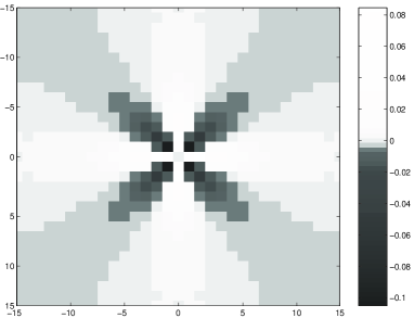
Figure 3: Perturbation of the shear stress field for a plastic event occurring at the origin in a medium submitted to a shear strain or stress.

III.2 Global effect of a plastic event :

We now consider more global effects of the same localized plastic event $\hat{\epsilon}_{xy}^{pl}({\bm{r}^{\prime}})=a^{2}\epsilon_{0}\delta({\bf r^{\prime}})$, namely quantities integrated over a whole layer (of constant $y$). The following integral rules are easily derived from the previous calculations:

$$\int^{+\infty}_{-\infty}\sigma_{xy}^{1}(x,y)dx = 0$$

$$\int^{+\infty}_{-\infty}u^{1}_{x}(x,y)dx = \mbox{Sign}(y)a^{2}\epsilon_{0}$$

$$\int^{+\infty}_{-\infty}u^{1}_{y}(x,y)dx = 0$$ (18)

The first equation states that the shear stress resulting from the plastic event is redistributed in such a way that the integrated stress on every layer is unchanged, i.e. there is no net release of stress over a layer, and consequently no change in the net force applied from above on the system! The second relation indicates that the average horizontal displacement in a (horizontal) layer depends only on whether it is above or below the event (but not on its distance to the event), while the third equation expresses that the average vertical displacement over a layer is zero. For simple shear in three dimensions, similar equations hold for quantities integrated over planes perpendicular to the loading displacement gradient.

III.3 Relation to other studies

Let us now compare the results we have obtained at the end of section A, for the displacement and stress fields induced by a single localized plastic event of simple shear symmetry, to related studies in the literature.

First, our results can be compared with the full analytical description of an elasto-plastic inclusion in an elastic matrix by Eshelby eshelby . In that study, plastic shear strain occurs only within the finite-sized inclusion which yields a perturbation of the shear stress around the inclusion. Whatever the explicit shape of the inclusion, the long-range behaviour of that perturbation is strictly identical to the equivalent for the 3D case of expression (14)(as we have checked).

To study collective effects, Baret et al. baret simulated elements with local yield stresses on a 2D-lattice (semi-periodic boundary conditions). In contrast with the present study, they modeled the plastic event by a simple scalar displacement. As a check, we computed the plastic strain tensor corresponding to such a local event in expression (11), and calculated the corresponding perturbed shear stress. This yields a perturbation of dipolar symmetry, consistent with the propagator that they numerically evaluated on their lattice. This provides a validation of our procedure, but mostly underlines that the nature and symmetry of the elementary plastic event seriously affect the propagator describing its consequences, and therefore potentially the collective interplay of such events and the resulting macroscopic flow behaviour. We believe that the form of plastic event used in the present study is more suited for the actual description of the flow of elastoplastic materials.

Kabla and Debrégeas kabla performed an explicit numerical simulation of a two dimensional foam under shear strain. In their quasi-static procedure, at each step the length of the film is minimized at constant bubble volume. They mimic ’T1’ event by reorganizing sets of four bubbles when film length decreases below a critical value. They studied the stress rearrangements following such T1 events in their simulation. Averaging over many such events, they found that statistically these stress perturbations have a quadrupolar symmetry ( with a slight tilt of the axes with respect to those of the macroscopic shear (x,y), probably due to a structuration of the foam by the flow into a slightly non-isotropic medium). They observed that this stress field coincides with that generated in an elastic medium by a set of dipoles with the orientation of the global forcing. What is remarkable is that the outcome of their cellular simulation is very consistent with the outcome of the (elastic) continuum approach followed here.

To describe the deformation of plastic amorphous materials, Langer has introduced the concept of introduces shear transformation zones (STZ). In langer1 , he studies the response of a 2D material to an applied deviatoric stress. The plastic strain tensor is described without any assumption on its orientation. The results in that paper suggest that for a plastic strain tensor with the symmetry of the forcing, the deviatoric stress induced by the STZ is of quadrupolar symmetry, with a power law decrease $\frac{1}{r^{4}}$. Within our model, we find for such an event also a quadrupolar symmetry but a power law decrease of $\frac{1}{r^{2}}$, and do not understand this discrepancy.

We now turn to the most important part of our paper, namely the effect of the finite-size geometry on the stress distortion due to a localized event.

IV Finite medium

As in the analysis above, we consider here localized plastic events with the symmetry of the forcing (simple shear), equivalent to a set of two dipoles of forces. Therefore the propagator for such a plastic event can in principle be viewed as the sum of the propagators for the four forces, which brings us back to considerations pertaining to the Green’s function for the effect of a single force on the elastic finite medium.

We focus on the case of an imposed shear strain represented on figure 4, where two solid walls adhering perfectly to the medium are shifted horizontally.

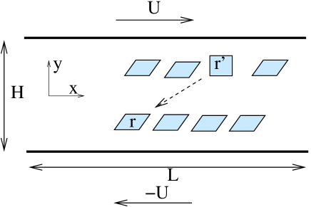
Figure 4: A shear strain $\frac{2U}{H}$ is applied to a two dimensional elasto-plastic medium. A plastic event occurs at position ${\bf r^{\prime}}$ and is here represented by a square, and we seek for the elastic deformation of the rest of the medium that will add up on the elastic loading symbolized by the parallelograms.

Therefore the boundary condition for the total displacement field is:

$${\bf u}(x,\pm H/2)=\pm{\bf U}$$ (19)

We proceed with the same decomposition as in the infinite medium case. The displacement field is the sum of the homogeneous elastic loading and of the perturbation due to the plastic event (again we denote by ${\bf u}^{1},{\bf\sigma}^{1}$ the displacement and deviatoric stress tensor induced by the plastic event). The boundary condition for the perturbation in the imposed strain regime is:

$${\bf u}^{1}(x,\pm H/2)={\bf 0}$$ (20)

The total response of the elasto-plastic medium is then :

$$u_{x}(x,y) = \frac{2Uy}{H}+u^{1}_{x}$$

$$u_{y}(x,y) = u^{1}_{y}$$

$$\sigma_{xy}(x,y) = \frac{2\mu U}{H}+\sigma^{1}_{xy}(x,y)$$

IV.1 Wall effects

We show here that the perturbation due to a plastic event occurring in the vicinity of a wall is more rapidly damped than the perturbation due to an elastic event occurring in the bulk.

To be precise, a plastic event is considered to occur in the vicinity of the bottom wall (located at $y_{w}=-H/2$) if it occurs at a position ${\bf r^{\prime}}$ much closer to the wall than the point ${\bf r}$ where the perturbation is calculated. This condition requires $|H/2+y^{\prime}|\ll|{\bf r-r^{\prime}}|$, with the notations defined on Figure 5. We also focus here on situations where the second (top) wall is too far to play a role, that is $|{\bf r-r^{\prime}}|\ll|{y^{\prime}-H/2}|$, so that our approach in this subsection practically deals with a semi-infinite geometry.

Figure 5: The plastic event occurs at the vicinity of the wall : $|{\bf r-r^{\prime}}|\gg d$. The quadrupolar symmetry of the plastic event is assumed not to be affected by the presence of the wall.

Again, the effect of a plastic event is equivalent to the sum of that of the four forces represented on Fig. 5. Hence, we first study the displacement field induced by a single force ${\bf F}$ at position ${\bf r^{\prime}}$ in the vicinity of the wall.

Figure 6: The displacement field due to a punctual force ${\bf F}$ in a semi infinite plane at a position ${\bf r^{\prime}}$ is the sum of the displacement field the same force would induce at ${\bf r^{\prime}}$ in an infinite medium, and that induced by its image with respect to the wall also in an infinite medium. The image consists of a punctual force ${\bf-F}$, two dipoles of forces of strength $2dF_{x}$ and $-2dF_{y}$ respectively, and two dipoles of potential. The resulting asymptotic long range behaviour is that of a quadrupole of strength $2dF_{x}$.

The displacement field due to a punctual force ${\bf F}$ at ${\bf r^{\prime}}$ in a semi infinite medium is the sum of the displacement field due to the punctual force and an image with respect to the wall in an infinite medium. This complex image is such that the displacement field it induces exactly cancel out on the wall the displacement generated by the punctual force. Its structure is depicted in Fig. 6 and recalled below pozri . The location of the image is the symmetric of the pole ${\bf r^{\prime}}$ with respect to the wall. This image is the sum of a punctual force $-{\bf F}$, two dipoles of forces $(2d{\bf e_{x}},F_{x}{\bf e_{y}})$ and ($2d{\bf e_{y}},F_{y}{\bf e_{y}}$), and two dipoles of potential ($2d{\bf e_{x}},F_{x}d/\mu$) and ($2d{\bf e_{y}},-F_{y}d/\mu$) where $d=|y^{\prime}+H/2|$ is the distance between the event and the wall. The analytical expression for the corresponding Green function is given in pozri . Its long-range behaviour, $|{\bf r-r^{\prime}}|\gg d$, is dictated by the dipoles of forces in Figure 6, yielding a displacement field that scales a $\frac{1}{|{\bf r-r^{\prime}}|}$.

Figure 7: The displacement field due to two force dipoles in a semi infinite plane is the sum of (i) the displacement field it would induce in an infinite medium and (ii) the displacement field due to its image with respect to the wall. This image can be constructed by summing those of the four forces. The contributions represented here (not at scale) are the direct images (solid arrows, all of amplitude $F$) and the induced force dipoles (dashed arrows, of amplitude $2(d-a)F$ and $2(d+a)F$ for the top and bottom one, of amplitude $2dF$ for the two others). Inspection shows that the net dominant long-range behaviour is that of a quadrupole twice as strong as the original one

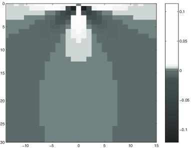
Figure 8: Perturbation of the shear stress field for a plastic event (plastic deformation of amplitude $\epsilon_{0}=1$) occurring next to the top wall.

Returning to the effect of a plastic event, where the source is now a set of dipoles as in Figure 2, one could expect a similar cancellation of the first order terms, and thus a far-field displacement scaling as $\frac{1}{|{\bf r-r^{\prime}}|^{2}}$. However inspection of the structure of the image show that such is not the case (see Figure 7): the dipole of horizontal forces is duplicated in its direct image, and the set of dipoles of vertical forces it generates yield a dipole of strength $4aF$. The contributions of the (original) dipole of vertical forces are weaker due to cancelations. Altogether one is left with a dominant term that has the same geometry than in an infinite medium (and a similar $1/r$ decay for the displacement) with an amplitude twice as strong. We have analytically checked that the stress decay is consistent with the above picture, as for a localized event close to the wall we obtain a propagator that is directly related to its equivalent in the absence of the wall Eq. (17) :

$$G_{\rm wall}(r,\theta)=2G^{\infty}(r,\theta)(1+O(d/r))$$ (22)

where clearly $x-x^{\prime}=r\cos(\theta)$ , $y-y^{\prime}=r\sin(\theta)$. This picture is also consistent with numerical calculations of the propagator for an event next to the wall in a finite geometry, which yields the picture in Fig. 8 (calculation to be described in subsection IVB below).

IV.2 Propagator in a finite thickness medium

In this subsection, we turn to a medium of finite thickness $H$. We focus again on an imposed strain situation, and therefore on the problem corresponding to the system of equation (III) together with the no displacement boundary conditions (20). We indicate ways of calculating the propagator in this geometry but mostly emphasize consequences of a single event on integral quantities.

IV.2.1 Finite $H$, Infinite $L$

A first method to treat the case of a medium of finite thickness and infinite length, consists in the systematic construction of a series of images so as to cancel the displacements on both walls.

In the previous subsection we reported the explicit structure of the image of a punctual force needed to cancel the displacement due to this force on one of the walls. The image with respect to the wall at $H/2$, unfortunately creates a displacement at the wall $-H/2$, so that its own image with respect to the wall $-H/2$ has to be considered, and this process has to be repeated for every image. Thus formally two infinite sums of images are required to express the displacement for a punctual force within two walls. Following this strategy, Pozrikidis pozri performed a full analytical calculation of the deformation field induced by a point force.

Formally, the perturbation due to a plastic event can then be deduced by adding up the consequences of each of the four forces it consists of. This leads to expressions that although exact are heavy to deal with and somewhat opaque. We therefore turn to other methods in the following, focusing on a geometry periodic in the $x$ direction.

IV.2.2 Finite $H$, $L$ Periodic : first method

Figure 9: A periodic array of plastic events at position $x^{\prime}+kL,y^{\prime}$.

We now focus on a system of thickness $H$ and of finite extent $L$ in the $x$ direction, and consider periodic boundary conditions in that direction. This is equivalent to analyzing in an unbounded geometry the effect of a periodic array of plastic events of a given amplitude at positions $(x^{\prime}+kL,y^{\prime})$ with $k\in\mathbb{Z}$ (Figure 9), or formally $\hat{\epsilon}_{xy}^{pl}({\bm{r}})=a^{2}\epsilon_{0}\sum_{k\in\mathbb{Z}}\delta({\bf r}-({\bm{r}^{\prime}}+kL{\bm{x}}))$. The resulting displacement field ${\bf u}^{1}$ can then be viewed as the sum of the displacement field induced by a similar periodic array of plastic events in an infinitely thick medium ${\bf u}^{\infty}$ and of a correction term ${\bf v}^{H}$ due to the finite size $H$. ${\bf u}^{1}={\bf u}^{\infty}+{\bf v}^{H}$ is a function of $x-x^{\prime},y\mbox{\, and \,}y^{\prime}$.

The displacement field ${\bf u}^{\infty}$ induced by the periodic array of plastic events in an infinite medium can be expressed using the propagator for a single event (14) :

$${\bf u}^{\infty}(x,y)=a^{2}\epsilon_{0}\sum_{k\in\mathbb{Z}}{\bf P}^{\infty}(x-x^{\prime}-kL,y^{\prime})$$ (23)

Given its periodicity in the $x$ direction, this expression can be formally decomposed in Fourier series:

$${\bf u}^{\infty}(x,y)={\bf U}_{0}^{\infty}(y)+\sum_{n=1}^{\infty} (\,{\bf U}_{cn}^{\infty}(y)\cos(2n\pi x/L)$$

$$+ {\bf U}_{sn}^{\infty}(y)\sin(2n\pi x/L)\,)$$

From equation (18), the components of the zeroth-mode vector function are:

$$U^{\infty}_{0x}(y) = \mbox{\,Sign\,}(y-y^{\prime})a^{2}\epsilon_{0}/L$$

$$U^{\infty}_{0y}(y) = 0$$ (25)

The correction displacement field ${\bf v}^{H}$ is the solution of incompressible linear elasticity with no source (i.e. the set of equations (3,4) with no plasticity) but with the boundary conditions required to grant that ${\bf u}^{1}$ is zero on the walls:

$${\bf v}^{H}(x,\pm H/2)+{\bf u}^{\infty}(x,\pm H/2)=0$$ (26)

${\bf v}^{H}$ is thus also periodic and can be written :

$${\bf v}^{H}(x,y)={\bf V}_{0}^{H}(y)+\sum_{n=1}^{\infty} (\,{\bf V}_{cn}^{H}(y) \cos(2n\pi x/L)$$

$$+ {\bf V}_{sn}^{H}(y) \sin(2n\pi x/L)\,)$$

where the functions ${\bf V}_{cn}^{H}$, ${\bf V}_{sn}^{H}$ can be calculated independently (i.e mode by mode) with the boundary conditions: ${\bf V}_{cn}^{H}(\pm H/2)=-{\bf U}_{cn}^{\infty}(\pm H/2)$, ${\bf V}_{sn}^{H}(\pm H/2)=-{\bf U}_{sn}^{\infty}(\pm H/2)$. We skip the full calculation in this subsection (which can be performed e.g. as in the low Reynolds number hydrodynamic study in Ajd ), as we display in the next subsection an exact expression of the displacement calculated in a framework that is more amenable to numerical simulation.

Instead we focus here on the zeroth mode ${\bf V}_{0}^{H}(y)$. From equations (IV.2.2) and (26), its components are simply:

$$V^{H}_{0x}(y) = -2a^{2}\epsilon_{0}\frac{y}{HL}$$

$${V}^{H}_{0y}(y) = 0.$$ (27)

This suffices to deduce consequences of the plastic event in terms of integrals over constant $y$ lines:

$$\int^{L/2}_{-L/2}{\bf u}^{1}dx=L({\bf V}_{0}^{H}(y)+{\bf U}_{0}^{\infty}(y))$$

so that

$$\int^{L/2}_{-L/2}u^{1}_{x}(x,y)dx = -2(a^{2}\epsilon_{0}\frac{y}{H})+\mbox{Sign}(y-y^{\prime})a^{2}\epsilon_{0}$$

$$\int^{L/2}_{-L/2}u^{1}_{y}(x,y)dx = 0$$

Then, linear elasticity implies that the overall variation of the force on the top plate due to the plastic event is:

$$\delta F=\int^{L/2}_{-L/2}{\sigma_{xy}}^{1}dx=-2\frac{\mu\epsilon_{0}a^{2}}{H}$$ (28)

The corresponding drop of the average shear stress in the medium is obviously $\delta\langle\sigma\rangle=\delta F/L$.

This exact expression shows that a single plastic event (of a given fixed amplitude $\epsilon_{0}a^{2}$) results in the release of the net force exerted by the medium on the walls by a quantity scaling as $\frac{1}{H}$. Remarkably, this quantity is independent on the position of the event in the medium. A corollary is that a finite density of plastic events $\phi$, will relax this total force by an amount $\sim(\phi HL)\delta F$, corresponding to a relaxation of the average stress $\delta\langle\sigma\rangle=\delta F/L$ independent of the size of the system.

Note that the integrals over a period $L$ calculated above for the consequences of a periodic array of plastic events, are equal to the integrals over $x$ from $-\infty$ to $+\infty$ in a finite $H$ infinite $L$ geometry for the consequences of a single plastic event. For example, in the latter geometry $\delta F=\int^{\infty}_{-\infty}{\sigma_{xy}}^{1}dx=-2\frac{\mu\epsilon_{0}a^{2}}{H}$, which clarifies in what sense equation (18) obtained in the previous section for an infinite medium corresponds to the limit $H\rightarrow\infty$. The global relaxation due to a single plastic event is consequently directly related to the finite size of the system.

An alternative derivation of this finite-size dependence of the force (or average stress) relaxation is proposed in appendix A, which yields a somewhat complementary physical insight.

IV.2.3 Finite $H$, $L$ Periodic : second method

Although we aim to focus in this paper on the qualitative aspects presented previously, we propose here an explicit formula for the stress perturbation induced by a localized plastic event in a finite size geometry. The actual expression is presented in reciprocal space, which may appear at first somewhat cumbersome, but turns out to be convenient in numerical calculations. For sake of readability, we provide here only the principles of this two step derivation and the resulting formulae, the details of the calculations being presented in appendix B.

First step: we formally extend the actual system ($0<y<H$, and $L$ periodic along $x$) by the following two operations: first an antisymmetric image system is constructed that extends to $-H<y<0$, then the $2H$ thick resulting system is repeated periodically in the $y$ direction. If the plastic strain in the original system is $\epsilon^{pl}(x,y)$, our construction yields a system without walls that is $2H$ periodic in the $y$ direction, with in the upper half period $H>y>0$ a plastic strain $\epsilon^{pl*}(x,y)=\epsilon^{pl}(x,y)$, and in the lower half $-H<y<0$ an antisymmetric image plastic strain $\epsilon^{pl*}(x,y)=-\epsilon^{pl}(x,-y)$. This construction ensures that the overall displacement generated by these strains has an $x$ component that is symmetric by reflection by the planes $y=0$ and $y=H$, and an $y$ component that is antisymmetric in the same operations. We have therefore generated a solution that satisfies the condition of a zero $y$ component of the displacement on the $y=0$ and $y=H$ planes (loci of the walls in the original system).

Second step: We now want to cancel the remaining displacements along $x$ without modifying the above result, and without adding sources in the system $0<y<H$. This can be achieved by adding on the planes $y=0$ and $y=H$ appropriate force fields $f_{x}$ directed along $x$ (again asymmetric and $2H$ periodic along $y$). Given the symmetry and periodicity of the system it is clear that the $y$ displacement on the walls is not modified by this addition.

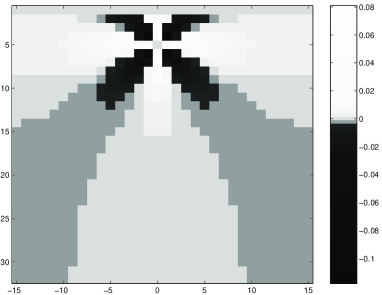
Figure 10: Perturbation of the shear stress field for a plastic event (plastic deformation of amplitude $\epsilon_{0}a^{2}=1$) occurring in the vicinity the wall. The discretization corresponds to $H/a=L/a=32$

When this is achieved, we have in the upper half $0<y<H$, a solution to (III) that satisfies the no displacement boundary condition on the walls (20). The corresponding stress field can be expressed in Fourier series :

$$\sigma^{1}(x,y)=\sum_{m,n\in\cal{Z}}e^{ip_{m}x}e^{iq_{n}y}\hat{\sigma}^{*}(m,n)\\$$

with $p_{m}=\frac{2\pi m}{L}$ and $q_{n}=\frac{2\pi n}{2H}$. It is the sum of the term directly generated by the plastic strains ${\hat{\epsilon}}^{*}$ and that due to the added force fields:

$$\hat{\sigma}^{*}(m,n) = 2\mu\{\hat{G}^{\infty}(m,n)\hat{\epsilon}^{pl*}(m,n)$$

$$+ \frac{1}{2}({\it i}p_{m}\hat{O}_{xy}(m,n)+{\it i}q_{n}\hat{O}_{xx}(m,n))\hat{f}_{x}(m,n)\}$$

$$\hat{\sigma}^{*}(0,0) = 0$$ (29)

The propagator $G^{\infty}$ and the Oseen tensor $\bf{O}$ are the direct counterparts for periodic systems of those defined in section III. Of course the force field $f_{x}$ in the above expression is itself proportional to the plastic strain; the corresponding formulae are given in appendix B.

Inverting back to real space allows to compute numerically the response to a localized event. We have checked that for a large system the stress created by a plastic event far from the walls according to this formula is close to that obtained analytically in section III for an infinite medium. Similarly, for an event directly neighbour to the wall, we recover the results of subsection IVA for a semi-infinite medium. Fig. 10 represents an intermediate situation : the event occurs in the vicinity of the wall.

V Conclusions and perspectives

Starting from a general elasto-plastic model, we have computed in different 2D geometries the modification of the shear stress resulting from a localized plastic event with a symmetry of simple shear. We have first calculated the corresponding perturbation in an infinite system forced with a symmetry of shear. The stress field is of quadrupolar symmetry and decreases with a power law $\frac{1}{r^{2}}$ in two dimensions. Then, we showed that the stress field perturbation due to a plastic event occurring close to a wall has a modified near field structure but decays far away with the same law and pattern, although with an amplitude twice as large. Eventually, we have proposed two ways of calculating the perturbation of the stress field due to a plastic event occurring in a finite medium. The first one allowed us to demonstrate in a simple way that a plastic event of a given strain amplitude relaxes the average stress by an amount which is independent of its position (i.e. distance to the walls) and inversely proportional to the size of the system. The second one allowed us to derive explicit expressions that permits calculation of the whole stress field in a finite-size geometry.

The extension of our results to a three dimensional situation is rather straightforward, and the qualitative statements are obviously similar. Also we have focused on a scalar description of plastic strain and induced stress, but the same steps can be taken if one seeks to describe the whole tensorial stress field generated by plastic events of arbitrary symmetry. Eventually, we have focused in section IV on a situation where the walls were kept fixed during the plastic event. The extension of our results to situations where the force on the plates is kept fixed is immediate: one simply needs to add to our solution a simple shear displacement (corresponding to a stress $-\delta F/L$ with the notations of section IV).

This study is meant to be a first step towards the modeling of the flow of an elasto-plastic material. The next one consists in plugging in a plastic law that describes the onset and evolution of the localized plastic events. Coupling such a local plastic behavior to the long-range elasticity described here should yield interesting collective behaviours and hopefully insights in the flow mechanisms. For such an endeavour our quantification of finite-size effects is important for the steady-state average balance between the stress released by the plastic events and that imposed by the elastic loading. Also the geometry and decay law of the elastic perturbation is to be considered when addressing the emergence of a collective/cooperative organization at low shear rates. Important questions regarding possible spatial and temporal heterogeneities in such flows (pignon ; varnik ; cous ; deb ; kabla could be addressed at the light of the present results:
- We have shown that a localized plastic event relaxes the average stress but also modifies the stress pattern on all the lines of the system decreasing the stress of some elements but increasing that of others. Does this allow shear banding with a limited zone flowing in coexistence with a non flowing region ?
- The average stress released during an event of given strain amplitude is independent of the position of the event in the medium, and is the same on all lines. Yet the geometry of the propagator is clearly modified by the proximity of a wall. Do these elements favor a localization of the flow at the wall ?
These questions will be addressed in a forthcoming publication.

Appendix A Finite size effects.

We propose an alternative simple approach which gives a different physical insight into the effects of finite size evidenced subsection IV.2. The following argument holds equally for an infinite $L\rightarrow\infty$ geometry or for an $L$ periodic medium, and is here presented for the latter. We consider a plastic event occurring at $(x^{\prime},y^{\prime})$ described by $\epsilon^{pl}_{xy}(x,y)=\epsilon_{o}a^{2}\delta(x-x^{\prime},y-y^{\prime})$ (and its repeated images along $x$ due to the $L$ periodicity). The stress perturbation is:

$$\sigma_{xy}^{1}(x,y)=\int^{L/2}_{-L/2}\!\!\!\!\!\!\!\!dx_{1}\int^{H/2}_{-H/2}\!\!\!\!\!\!\!\!dy_{1}\,G^{HL}(x-x_{1},y,y_{1})\epsilon_{xy}^{pl}(x_{1},y_{1})$$ (30)

which actually defines the propagator $G^{HL}$ for the present periodic medium. The corresponding force release on the bottom of a layer at height $y$ is

$$\delta F=\int^{L/2}_{-L/2}\!\!\!\!\!\!dx\,\,\sigma_{xy}^{1}(x,y)=a^{2}\epsilon_{0}\int^{L/2}_{-L/2}\!\!\!\!\!\!dx\,\,G^{HL}(x-x^{\prime},y,y^{\prime})$$ (31)

We remark that this can be rewritten

$$\delta F=\int^{L/2}_{-L/2}\!\!\!\!\!\!\!\!dx_{1}\int^{H/2}_{-H/2}\!\!\!\!\!\!\!\!dy_{1}\,G^{HL}(x-x_{1},y,y_{1})(\epsilon_{0}a^{2}\delta(y_{1}-y^{\prime}))$$ (32)

which means (see (A1)) that the variation of the integrated stress over a layer at height $y$ ($\delta F$) induced by an event occurring at position $x^{\prime},y^{\prime}$, is equal to the stress variation at a site $(x^{\prime},y)$ induced by a continuous sum of events on a layer $y^{\prime}$.

Representing these events by pairs of dipoles, the sum reduces to that of the $x$ components as the $y$ components cancel out upon summation on the line, so that we are looking for the stress generated at $(x^{\prime},y)$ by the two lines of forces at $y^{\prime}-a$ and $y^{\prime}+a$ depicted on Figure 11.

Figure 11: Left: a continuous line of events at height $y^{\prime}$ is equivalent, using the representation of Figure 2 for a single event, to two lines of horizontal forces at $y^{\prime}+a$ and $y^{\prime}-a$. Right: displacement profiles resulting from the sum of negative forces at $y^{\prime}-a$ (left), and from the sum of positive forces at height $y^{\prime}+a$ (right).

The displacement field resulting from each of these sums separately are easily calculated and depicted on the right of Figure 11. For example the second one is the solution of the following problem: on each side of the plane $y=y^{\prime}-a$, the medium is purely elastic, with no displacement at the walls, and at $y=y^{\prime}-a$ a continuous displacement and a jump in the stress of amplitude $\mu\epsilon_{0}a$.

The total effect of the continuous line of events is the displacement field presented on the left of Figure 12. The slopes of the profile for $y>y^{\prime}+a$, and $y<y^{\prime}-a$ are the same, and correspond to $\delta F=-2\frac{\mu\epsilon_{0}a^{2}}{H}$, as derived differently in the main text, see equation (28). Remarkably, this value, which corresponds to the force release on the top wall, is independent of the position of the plastic event.

Figure 12: Left : displacement profile due to the line of events at $y^{\prime}$ (obtained by summing the two profiles of Fig. 11 right), and schematic description of the elastic loading. Right: total response to the global forcing and a line of plastic event (a homogeneous fracture), obtained by summing the two profiles on the left.

We remark that the deformation profile obtained here is very similar to the one obtained by Kabla and Debrégeas in their explicit simulation of a shear foam kabla (which in their case was the line average consequences of a single local event, equivalent to the present local consequence of a line of events according to the argument below (A3)).

As a follow-up along the same picture, the cumulative displacement after loading plus a continuous line of plastic events is represented on the right of Figure 12 : the total shear in the system is then the homogeneous shear due to the forcing minus the shear release due to the plastic events.

Appendix B Stress field induced by a plastic deformation in a finite medium

In this appendix we provide the explicit derivation of the stress field change due to a plastic activity in a finite system, follow the strategy outlined in subsection IVB.3. The aim is to obtain the response of the system depicted on figure 9 to a strain solicitation $\epsilon^{pl}(x,y)$ with ”stick” boundary conditions on the wall similar to 20. For this calculation we choose to take the origin of the $y$ axis on the bottom wall so that the walls (and thus the boundary conditions) are at $y=0$ and $y=H$.

Figure 13: Auxiliary system corresponding to the real system of figure 9: it is periodic in both direction and symmetric in the $y$ direction. The driving plastic strain field $\epsilon^{pl*}$ is antisymmetric.

Geometry of the auxiliary system-

To solve this problem, an auxiliary system with no walls is constructed. Its geometry is that of the original system, symmetrized with respect to $y=0$, and periodized along $y$. The new system has thus a period $L$ in the $x$ direction, and a period $2H$ in the $y$ direction, see Fig. 13. Fields in this new system are described by stars. The symmetry with respect to the plane $y=0$ is made in such a way that the plastic strain is antisymmetric $\epsilon^{pl*}(x,-y)=-\epsilon^{pl*}(x,y)$, which is equivalent in the force dipole representations to having the force fields in the lower half to be the symmetric of that in the upper part $\bm{F}^{*}(x,y)=\bm{F}^{*}(x,-y)$. The symmetry and periodicity of the problem ensures that the displacement field $\bf{u}^{*}$ generated by this plastic strain satisfies verify by symmetry and periodicity :

$$u_{y}^{*}(x,0)=0;u_{y}^{*}(x,H)=0$$ (33)

Response to a plastic event-

This new elastic system is submitted to a plastic strain $\epsilon^{pl*}(x,y)=\epsilon^{pl}(x,y)\mbox{\, if \,}y>0$, and $\epsilon^{pl*}(x,y)=-\epsilon^{pl}(x,-y)\mbox{ \, if \,}y<0$. For reasons explained in the text (section IVB.3), a force field $f_{x}^{*}$ is added at the location of the walls in the real system, to cancel the displacements $u_{x}(x,0)$ and $u_{x}(x,H)$ created by the plastic strains.

$$f_{x}^{*}(x,y)=f_{0}^{*}(x)\delta(y)+f_{H}^{*}(x)\delta(y-H)$$ (34)

This ”no displacement on planes $y=0$ and $y=H$” condition is implemented in reciprocal space. We introduce notations for the Fourier series:

$$\bm{u}^{*}(x,y) = \sum_{m,n\in\cal{Z}}e^{i\frac{2\pi mx}{L}}e^{i\frac{2\pi ny}{2H}}\hat{\bm{u}}^{*}(m,n)$$

$$\hat{\bm{u}}^{*}(m,n) = \frac{1}{2HL}\int\!dxdy\,\bm{u}^{*}(x,y)\,e^{-i\frac{2\pi mx}{L}}e^{-i\frac{2\pi ny}{2H}}$$

$$p_{m}=\frac{2\pi m}{L} q_{n}=\frac{2\pi n}{2H};\,q^{2}=p_{m}^{2}+q_{n}^{2}$$ ;

From our calculations for an infinite medium in section III, it is logical to write the total displacement using propagators for plastic events and the Oseen propagator for simple forces:

$$\hat{\bm{u}}^{*}(m,n) = \hat{\bm{P}}^{\infty}(m,n)\hat{\epsilon}^{pl*}(m,n)$$ (36)

$$+ \hat{\bm{O}}(m,n)\hat{f}_{x}(m,n)$$

The equations for $\bm{P}^{\infty}$ and the Oseen tensor $\bm{O}$ in the present representation (Fourier series) are formally exactly similar to those obtained in (III) and (14) in terms of Fourier transforms (with $q_{x}\rightarrow p_{m}$ and $q_{y}\rightarrow q_{n}$).

The condition $u^{*}(x,0)=0;u^{*}(x,H)=0$ allows to compute $\hat{f}^{*}_{x}(m,n)$.

$$\hat{f}^{*}_{x}(m,n) = \frac{\sum_{1}\frac{2i}{q^{4}}p_{n}^{\prime}(q_{m}^{2}-p_{n}^{\prime 2})\hat{\epsilon}^{pl*}(m,n^{\prime})}{\sum_{1}\frac{p_{n}^{\prime 2}}{\mu q^{4}}},$$

for odd n

$$\hat{f}^{*}_{x}(m,n) = \frac{\sum_{2}\frac{2i}{q^{4}}p_{n}^{\prime}(q_{m}^{2}-p_{n}^{\prime 2})\hat{\epsilon}^{pl*}(m,n^{\prime})}{\sum_{2}\frac{p_{n}^{\prime 2}}{\mu q^{4}}},$$

$$\mbox{for even n and \,}m\neq 0$$

$$\hat{f}^{*}_{x}(0,n) = 0\mbox{ \, for even n}$$

$\sum_{1}$ describes the sum over odd values of $n^{\prime}$, and $\sum_{2}$ the sum over even values of $n^{\prime}$.
The shear stress in this geometry can then be derived from the displacement field:

$$\hat{\sigma}^{*}(m,n)=2\mu(\frac{1}{2}({\it i}p_{m}\hat{u}^{*}_{y}(m,n)+{\it i}q_{n}\hat{u}^{*}_{x}(m,n)-\hat{\epsilon}^{pl*}(m,n))$$ (37)

For symmetry reasons, $\hat{\sigma*}(0,0)=0$.

Back to the real system -

The displacement field $\bf{u}^{*}(x,y)$ that we have constructed and computed satisfies the elasticity equations for $H>y>0$ with the plastic strain $\epsilon^{pl}(x,y)$ as only source in that area, and verifies the boundary conditions $u^{*}(x,0)=0$ and $u^{*}(x,H)=0$. It is therefore the solution to our initial problem for the real system: for $H>y>0$, $\bf{u}^{1}(x,y)=\bf{u}^{*}(x,y)$, and $\sigma^{1}(x,y)=\sigma^{*}(x,y)$. Hence, the expression of the stress as given in Equation (29).

References

- (1) Author for correspondance: armand.ajdari@espci.fr
- (2) L.J. Chen, B.J. Ackerson, and C.F. Zulowski, J. Rheol. 38,193 (1993).
- (3) F. Pignon, A. Magnin, and J.-M. Piau, J. Rheol. 40,573 (1996).
- (4) F. Varnik, L. Bocquet, J.-L. Barrat, L. Berthier, Phys. Rev. Lett. 90, 095702 (2003).
- (5) P. Coussot et al., Phys. Rev. Lett., 88, 218301 (2002).
- (6) G. Debrégeas, H. Tabuteau, and J.-M. di Meglio, Phys. Rev. Lett. 87, 178305 (2001).
- (7) K. Chen, P.Bak, Obukhov, Phys. Rev. A 43,625, (1991).
- (8) V.V. Bulatov and A.S. Argon, Modell. Simul. Mater. Sci. Eng. 2, 167 (1994).
- (9) V.V. Bulatov and A.S. Argon, Modell. Simul. Mater. Sci. Eng. 2, 185 (1994).
- (10) V.V. Bulatov and A.S. Argon, Modell. Simul. Mater. Sci. Eng. 2, 203 (1994).
- (11) M.L. Falk and J.S. Langer, Phys. Rev. E 57, 7192, (1998).
- (12) J.S. Langer, Phys. Rev. E 64, 011504, (2001).
- (13) J. C. Baret, D. Vandembroucq, S. Roux, Phys. Rev. Lett. 89, 195506 (2002).
- (14) O.M. Braun, J. Roder, Phys. Rev. Lett. 88, 096102 (2002).
- (15) J.D. Eshelby, Proc. R. Soc. London, Ser. A 241,376 (1957).
- (16) A. Kabla, G. Debrégeas, Phys. Rev. Lett. 90, 258303 (2003)
- (17) C. Pozrikidis, Boundary Integral and Singularity Methods for Linearized Viscous Flow. Cambridge University Press (1992).
- (18) A. Ajdari, Phys. Rev. E, 53, 4996-5005 (1996).