The Magnetic Ordering of the 3d Wigner Crystal

Abstract

Using Path Integral Monte Carlo, we have calculated exchange frequencies as electrons undergo ring exchanges of 2, 3 and 4 electrons in a “clean” 3d Wigner crystal (bcc lattice) as a function of density. We find pair exchange dominates and estimate the critical temperature for the transition to antiferromagnetic ordering to be roughly $1\times 10^{-8}$Ry at melting. In contrast to the situation in 2d, the 3d Wigner crystal is different from the solid bcc ³He in that the pair exchange dominates because of the softer interparticle potential. We discuss implications for the magnetic phase diagram of the electron gas.

I Introduction

The uniform system of electrons is one of the basic models of condensed matter physics. Wignerwigner pointed out that at low density, the potential energy dominates and the system will form what is now called a Wigner crystal (3dWC). There have been attempts to make laboratory examples of the low density homogeneous 3d electron gas with specially designed band-engineered AlGaAs heterostructuressuper . In this paper, we report on calculations of the spin Hamiltonian in the low density 3d Wigner crystal.

At $T=0$, the properties of the electron gas are determined by a single dimensionless parameter $r_{s}=a/a_{0}=(m^{*}/m\epsilon)a/a_{b}$ where $a=(3/4\pi\rho)^{1/3}$, $a_{b}$ is the Bohr radius, $m^{*}$ is the effective mass, and $\epsilon$ the dielectric constant. In this paper we will use effective Rydbergs for energies Ry${}^{*}=(m^{*}/m_{e}\epsilon^{2})$Ry and $a$ for units of length. In these units the Hamiltonian is:

$$H=-\sum_{i}\frac{1}{r_{s}^{2}}\nabla_{i}^{2}+\frac{2}{r_{s}}\sum_{i,j}\frac{1}{r_{i,j}}.$$ (1)

Though a variety of methods have been applied to calculate the properties of the low density electron system, the most successful have been direct simulation methods: namely Quantum Monte Carlo. Ceperley and AlderCA80 using Diffusion Monte Carlo (DMC) determined that melting at zero temperature occurs at $r_{s}\simeq 100\pm 20$ for spin 1/2 fermions, and at $r_{s}\simeq 160$ for bosons. (This is also the zero temperature melting density for distinguishable particles). Later estimatesortiz found melting at higher densities ($r_{s}=65\pm 10$), but the variational trial functions in the liquid phase were not sufficiently accurate. Very recently, Drummond et al.needs04 confirmed the estimate of $r_{s}=106\pm 1$ using DMC with a variety of better functions and the more accurate results of Zong et al.zong02 in the fluid phase. The bcc crystal structure has the lowest energy throughout the stability region of the crystal. See, for example, the QMC calculations of Harris et al.ortiz who found bcc the lowest energy structure in the range $r_{s}>60$.

Once the melting density is established, it is of interest to determine the low temperature spin order. Harris et al.ortiz reported finding the ferromagnetic bcc phase as stable, however, other aspects of those calculations have not been reproduced. Drummond et al.needs04 attempted to determine directly the energy difference between ferromagnetic and antiferromagnetic orderings using DMC but found the difference zero within their error bars (on the order of $2\times 10^{-7}$Ry at $r_{s}=100$). This is consistent with the results reported below. One needs to use a method sensitive to the small magnetic energies, which are typically many orders of magnitude smaller than the plasmon energies that determine the accuracy of the DMC energies.

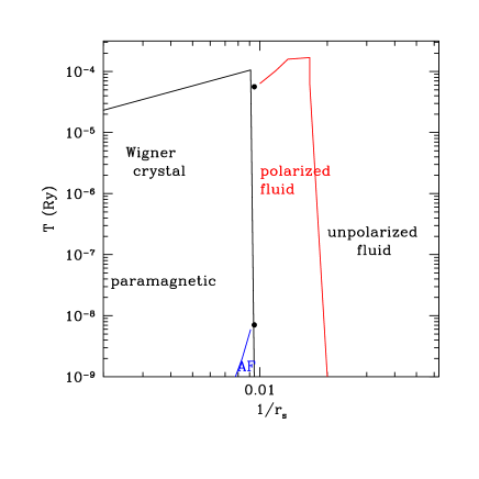
Figure 1: Phase diagram of the 3d electron gas showing the region of stability of the crystaljones , the polarization transition from QMC calculationszong02 and the antiferromagnetic transition (this work). (color online)

Jones and Ceperleyjones studied the quantum melting curve for distinguishable particles. At densities for $r_{s}\geq 100$ the melting is classical, and occurs for temperaturescocp $k_{B}T_{melt}=2/(\Gamma_{c}r_{s})$Ry where $\Gamma_{c}\approx 173$. We only use this melting to determine the region where the crystal is stable, and thus the region where magnetic ordering is relevant. Fig. 1 summarizes the 3deg phase diagram.

For spin 1/2 particles, the magnetic ordering is not fixed by the spatial ordering. The earliest quantitative calculation was using a Slater determinant of localized Wannier functions (i. e. Gaussians) by Carr.carr He found an antiferromagnetic phase in the Wigner crystal at intermediate density and ferromagnetic at lower density. We will compare with this calculation later in the paper. Edwards and Hilleledwards using a Hartree-Fock method with a flexible, delocalized basis and a variety of spin orderings found antiferromagnetic ordering at intermediate density $10<r_{s}<40$ and ferromagnetic at lower densities. But, as mentioned above, the crystal phase is only stable for $r_{s}>106$.

Herringherring reviewed the situation as understood in 1965 in some detail, including the contribution of ring exchanges of electrons. Thoulessthouless introduced the current theory of magnetism in quantum crystals. According to this theory, in the absence of point defects, at low temperatures the electrons will almost always be near a lattice site. If the system is constrained to stay in the neighborhood of the two perfect lattice positions $Z$ and $PZ$ where $P$ is a permutation of particle labels, the exchange frequency equals the splitting between the antisymmetric spatial state and the symmetric spatial state: $2J_{P}=E_{A}-E_{S}>0$. The spin Hamiltonian comes about from making the total wavefunction antisymmetric:

$${\mathcal{H}}_{spin}=-\sum_{P}(-1)^{P}J_{P}{\hat{\mathcal{P}}}_{spin}$$ (2)

where the sum is over all cyclic (ring) exchanges described by a cyclic permutation $P$, and ${\hat{\mathcal{P}}}_{spin}$ is the corresponding spin exchange operator. (Although more complex products of several ring exchanges are possible, in cases considered, they are negligible.) The sign, $(-1)^{P}$, implies that an exchange of even number of electrons is antiferromagnetic and an odd number of electrons is ferromagnetic. Ring exchange models have been used to describe correlated electron systems, such as high temperature superconductorshightc , quantum Hall systemskivelson as well as electrons2dWC and helium atomsrogerhe confined in planes.

One might expect that pair electron exchanges would dominate over higher-body exchanges. Since the bcc lattice is bipartite, a simple Néel antiferromagnetic state would seem to be favored. Rather surprisingly, it has been foundRHD that in 3d solid ³He, which also forms a bcc lattice, exchanges of 2, 3 and 4 particles have roughly the same order of magnitude and must all be taken into account to understand the magnetic ordering. This is known as the multiple spin exchange model(MSE). The resulting spin order is more complex since the order is frustrated by the competing exchanges. We wish to determine whether such a model is relevant for the 3dWC.

Figure 2 shows the pair correlation functions for solid ³He and the electron gas near the crystallization density. Because the $g(r)$’s are so similar, one might expect their exchanges frequencies would be similar and hence have the same magnetic ordering. We also note that the Lindemann’s ratio, the mean squared displacement in units of the nearest neighbor spacing, for bulk helium and the Wigner crystal are also similar near melting ($0.32$ and $0.30$ respectively). However, note the $g(r)$’s are very different at small $r$ because the potentials are so different; the helium-helium interaction is much more repulsive at short distances.

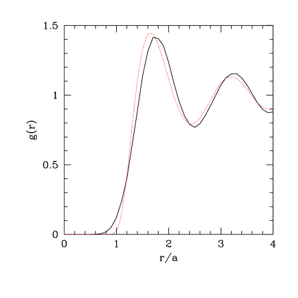
Figure 2: The pair correlation function for the 3dWC (solid line) ($r_{s}=100$) and for bcc ³He (dashed red line)also at melting ($24.23cm^{3}/mole$. The functions are nearly identical, though the electrons can get significantly closer together than helium atoms can. (color online)

In this paper, we determine the magnetic interaction in the Wigner crystal, based on Thouless’thouless theory of exchange. Path Integral Monte Carlo (PIMC) as suggested by Thoulessthouless and Rogerroger84 has proved to be a reliable way to calculate these parameters directly from the Coulomb interaction. The theory and computational method have been tested thoroughly on the magnetic properties of bulk helium obtaining agreement with measured propertiesRMPI . We2dWC have also used this method to calculate exchange frequencies in the 2dWC. Here we report results for the 3dWC.

II Computational Details

The Path Integral method for calculating exchange frequencies is based on the ratio:

$$f_{P}(\beta)=\frac{\langle Z|e^{-\beta H}|PZ\rangle}{\langle Z|e^{-\beta H}|Z\rangle}$$ (3)

where $Z$ represents the many-body configuration of electrons sitting on the bcc lattice sites and $PZ$ is a permutation of those sites. Then under general assumptions, the exchange frequencies are given by:

$$f_{P}(\beta)=\tanh(J_{P}(\beta-\beta_{0}))$$ (4)

where $\beta_{0}$ is the amount of imaginary time to initiate the exchange. The ratio $f_{P}$ is determined by a specialized Path Integral Monte Carlo method and Eq. 4 is inverted to determine $J_{P}$.

We do simulations with two types of paths: a) paths beginning and ending at the perfect lattice positions and b) paths beginning at $Z$ and ending at $PZ$. The imaginary time density matrices $e^{-\beta H}$ are expanded out into a path integral connecting the end-points of the paths. Using the polymer “isomorphism”RMPI , $f_{P}(z)$ is related to the free energy need to induce a specific cross-linking $P$ into a crystal of ring polymers. Using the Bennett methodbennett ; CJ , we directly determine the ratio $f_{P}$ by examining histograms of the change in action in mapping paths of one type into paths of the other type. With this method we can determine very small frequencies to an accuracy of a few percent, irrespective of the magnitude of $J_{P}$.

Ewald sums are used to represent the Coulomb interaction in periodic boundary conditions, taken as a cube. The potential is split into long-range and short-range terms with the usual Gaussian breakupceperley78 . Then the exact two particle action for the short ranged potential (the complementary error function) is determined using matrix squaring.RMPI The long range action is taken in the primitive approximation; this is appropriate since it is smooth. Most calculations were done with 54 electrons in the simulation cube with a few tests of 128 electrons giving agreement. Note that at low density, long wave-length plasmons are strongly suppressed by the potential energy, making the exchange more localized spatially than is the case with solid helium.

One numerical approximation is the imaginary-time step, or equivalently, the number of points on the path. We did several calculations for each value of $r_{s}$ and each type of exchange to establish that the results are in the zero time step limit within error bars. A second approximation concerns the value of $\beta$ in Eq. 3. Because the exchanges are instantons (i. e. confined in imaginary time), the results converge quickly in $\beta$ as long as $\beta_{0}<\beta$. We typically choose $\beta<3\beta_{0}$ and observe very weak dependance on $\beta$. Typically, for converged results, this implies one to two hundred steps in the exchange. Further details of the method have been discussed in earlier papers.cornell

In order to keep the system from melting for densities higher than the bosonic meltingCA80 $100\leq r_{s}\leq 160$, the electron paths are restricted to stay in the positive region of a trial wavefunction: the fixed-node boundary conditions. We separate the electrons into those exchanging (say “$p$” of them) and the spectators ( i. e. $N-p$ electrons). A Slater determinant of only the spectator electrons is constructed:

$$\psi(R(t))=\det[\exp(-c({\bf r}_{i}(t)-{\bf z}_{j})^{2})]$$ (5)

where ${\bf z}_{j}$ is the set of spectator lattice sites and ${\bf r}_{i}(t)$ the imaginary time path of the spectator electrons. The value of the parameter $c$ was optimized by variational Monte Carloceperley78 : $c=0.2r_{s}^{1/2}$. The more recent values obtained by minimizing the fixed-node energyneeds04 $c=0.11r_{s}^{1/2}$ were not available when we did the calculations. A Slater determinant of Gaussian orbitals is an accurate representation for the nodes of the many-electron ground state wavefunction. More complicated forms, such as linear combinations of Gaussians, do not result in a significantly better trial functionsneeds04 for the 3dWC.

Only paths which keep a positive determinant throughout the path are kept $\psi(t)>0$ for $0\leq t\leq\beta$: this is the fixed-node method. We find that these boundary conditions are sufficient to keep the system from melting. We do see a suppression of the exchange frequency caused by the determinantal boundary conditions at $r_{s}=150$ of about $10\%$. In principle, the spin ordering should be determined self consistently. For example, it would be better to apply antiferromagnetic boundary conditions, however, we have not tested that approach. For this reason, we may have corrections to the exchange frequencies on the order of 10%, particularly near melting.

III Exchange Frequencies

We have calculated 2, 3 and 4 particle exchanges for six different densities in the range $100\leq r_{s}\leq 150$. We determined two different pair exchanges: first neighbor, $J_{nn}$, and second neighbor, $J_{nnn}$. We do find a significant 2 body next-nearest-neighbor exchange. The most compact three-body exchange, $J_{t}$, has two first-neighbor and one second-neighbor electrons. There are two types of four electron exchanges involving only first neighborsRHD : the planar exchange, $J_{p}$, and the folded exchange, $J_{f}$. Table I shows the exchange frequencies of our calculations versus density.

Figure 3 shows the exchange frequencies versus density. We find that the exchange energies are very much smaller than the plasmon energies. The kinetic energy of the Wigner crystal can be expanded in a power seriesceperley78 :

$$T=-\frac{d(r_{s}E)}{dr_{s}}=0.669r_{s}^{-3/2}-0.553r_{s}^{-2}.$$ (6)

In the density range of consideration, the kinetic energy varies from 0.6 mRy to 0.3 mRy: five orders of magnitude greater than the exchange frequencies. Roughly speaking, the electrons vibrate around their lattice sites $10^{5}$ times before exchanging with a nearby electron. This is comparable with the situation in bcc ³He and justifies that we can reduce the original Hamiltonian involving charges, Eq. 1, to the spin Hamiltonian, Eq. 2.

We see in Fig. 3 that the exchange frequencies drop off exponentially: roughly as $\exp(-Sr_{s}^{1/2})$. This follows from assuming a single most probable path for the ring exchangeroger84 is independent of density. (Note that we do not make this assumption in the PIMC simulation). It is likely that WKB calculation of $S$ will give reasonable estimates of the exchange frequencies as they do for the 2dWCroger84 ; hirashima .

We find that the rate for pair exchanges is much larger than the other exchanges, making a very stable antiferromagnetic ground state. The planar 4-body exchange, also antiferromagnetic, is slightly larger than the ferromagnetic, 3-body exchange. Only ratios of the exchange rates can enter into determining the stability of a given magnetic state. Figure 4 shows the density dependance of the ratios $J_{f}/J_{n}$ and $J_{t}/J_{n}$. We see a decrease in these ratios as density decreases, thereby further stabilizing the antiferromagnetic phase. Next in importance is the 2-body next nearest neighbor exchange, followed by the folded 4-body exchange.

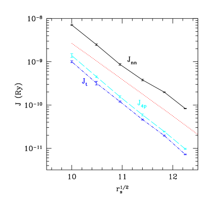
Figure 3: (color online) Exchange frequencies (in Ry log scale) versus $r_{s}^{1/2}$. The solid (black) line shows the 2-body nearest neighbor exchange. The dashed (red) line is from the calculations of Carrcarr . The other lines are the triple (blue short dashes) and planar 4-electron (cyan, long dashes) exchange frequencies. A WKB calculation would be a straight line.

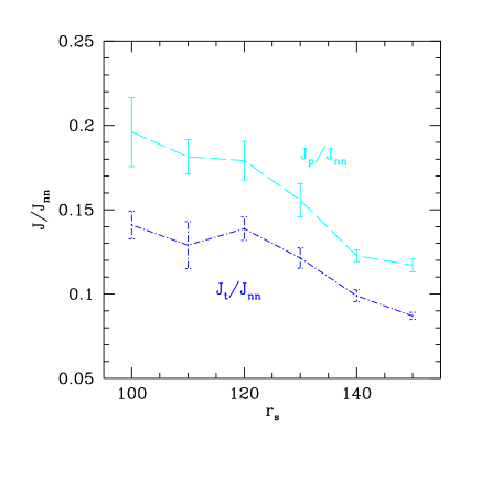
Figure 4: (color online) Ratio of exchange frequencies versus $r_{s}$. Shown are $J_{t}/J_{nn}$ (blue, short dashes) and $J_{p}/J_{nn}$ (cyan, long dashes).

Table 1: Results of the PIMC calculations at various values of $r_{s}$. Units are $10^{-9}$ Ry/electron. Quantities in () are the estimated relative statistical error. The second column is the estimated transition temperature (also in nRy) based on Eq. 13. The spin couplings $j_{n}$ are defined in Eq. 8.

$r_{s}$	$k_{B}T_{c}$	$J_{nn}$	$J_{nnn}$	$J_{t}$	$J_{p}$	$J_{f}$	$j_{1}$	$j_{2}$	$j_{3}$
		2 (11)	2 (22)	3 (112)	$4(1^{4};23)$	$4(1^{4};22)$
100	16.	7.09 (0.03)		1.0 (0.05)	1.39 (0.10)		5.6	-1.9	0.7
110	6.0	2.48 (0.05)		0.32 (0.10)	0.45 (0.04)		2.0	-0.6	0.2
120	2.0	0.865 (0.04)	0.058 (0.03)	0.12 (0.03)	0.155 (0.04)	0.0112( 0.05)	0.64	-0.25	0.08
130	0.90	0.379 (0.04)		0.0460 (0.03)	0.059 (0.05)	0.0037 (0.06)	0.29	-0.09	0.03
140	0.49	0.200 (0.04)		0.0196 (0.03)	0.0243 (0.02)		0.16	-0.04	0.01
150	0.21	0.0827 (.014)		0.00720 (0.02)	0.00968 (0.03)	0.000565 (0.025)	0.071	-0.014	0.005

IV Magnetic properties

Having determined the exchange frequencies, we can now discuss the magnetic properties, based on the spin Hamiltonian in Eq. 2. In principle, one has a formidable many-body problem. However, we can make use of the extensive results available from studies of solid ³He, also a bcc lattice. In particular, see the review of Roger et al. RHD (RHD) and references therein. For spin 1/2 particles, one can write the spin Hamiltonian in terms of Pauli spin matrices. Two and 3 particle exchanges map into a Heisenberg model:

$$H_{h}=\frac{j_{1}}{2}\sum_{i,j}^{(1)}{\mathbf{\sigma}}_{i}\cdot{\mathbf{\sigma}}_{j}+\frac{j_{2}}{2}\sum_{i,j}^{(2)}{\mathbf{\sigma}}_{i}\cdot{\mathbf{\sigma}}_{j}+\ldots$$ (7)

where the sums are over first, second and third neighbor pairs respectively. (Note on notation: $J_{x}>0$ refers to a ring exchange frequency for the cycle $x$, while $j_{n}$ refers to the coupling constant in Eq. 7 between two spins a distance $x$ apart; all frequencies have an opposite sign from the notation of RHD.) These spin couplings are given in terms of the ring exchanges by:

$$j_{1} = J_{nn}+3(-2J_{t}+J_{p}+J_{f})$$ (8)

$$j_{2} = 2(-2J_{t}+J_{f})+J_{p}+J_{nnn}$$

$$j_{3} = J_{p}/2.$$

The pair couplings, shown in Table I, can either be positive (antiferromagnetic) or negative (ferromagnetic) depending on the relative importance of even and odd ring exchanges.

The four spin exchanges lead to additional four spin terms in the effective Hamiltonian in Eq. 7.

$$G_{ijkl}=({\mathbf{\sigma}}_{i}\cdot{\mathbf{\sigma}}_{j})({\mathbf{\sigma}}_{k}\cdot{\mathbf{\sigma}}_{l})+({\mathbf{\sigma}}_{i}\cdot{\mathbf{\sigma}}_{l})({\mathbf{\sigma}}_{j}\cdot{\mathbf{\sigma}}_{k})-({\mathbf{\sigma}}_{i}\cdot{\mathbf{\sigma}}_{k})({\mathbf{\sigma}}_{j}\cdot{\mathbf{\sigma}}_{l})$$ (9)

$$\Delta H_{x}=\frac{J_{x}}{4}\sum_{i,j,k,l}G_{ijkl}.$$ (10)

The summation ($x=p$ or $x=f$) is over distinct labels describing the planar or folded four-particle exchanges. According to RHD, one can neglect these additional terms in estimating properties at high temperatures. Since they are fourth order in the order parameter field, they can only contribute at lower temperature.

Given the above spin Hamiltonian, several things can be easily computed. At high temperature, the Curie-Weiss constant measures the leading term in a $1/T$ expansion to the susceptibility ($\chi^{-1}=C(T-\Theta+B/T+\ldots)$. We find that:

$$\Theta=4J_{nn}+3J_{nnn}-36J_{t}+18K_{f}+18K_{p}.$$ (11)

In regions above the ordering temperature, this determines the deviation with respect to uncoupled spins. It is positive (antiferromagnetic), for all densities.

From the dominance of $J_{nnn}$ over the other ring exchanges, we expect ordering into an antiferromagnetic phase via a second order transition at a sufficiently low temperature. The complications resulting from a frustrated spin Hamiltonian are absent, so that we can be considerably more confident in our predictions than is the case with a frustrated spin-model such as helium or the 2dWC. First, let us determine the transition temperature within mean field theory. RHDRHD (Fig. 16) show the mean field phase diagram as a function of $(j_{1},j_{2},j_{3})$ As mentioned above, the four spin terms will not change this diagram. Based on the values in Table I, we find that the 3dWC is very much in the antiferromagnetic region. The density dependance shown in Fig. 4, has a tendency to enhance even more the antiferromagnetism at larger values of $r_{s}$.

Within mean field theory, the antiferromagnetic phase has a critical transition temperature:

$$k_{B}T_{c}=4j_{1}-3j_{2}-6j_{3}.$$ (12)

We can include fluctuations into this estimate by using results of series expansions. Oitmaa and Zhengoitmaa have calculated properties of the $j_{1},j_{2}$ model on a bcc lattice using Padé approximates to high temperature expansions (up to tenth order in the inverse temperature.) They find the antiferromagnetic phase is stable at low temperatures for $j_{2}\leq 0.705j_{1}$. They also find that the transition temperature is $k_{B}T_{c}\approx 2.76j_{1}-2.61j_{2}$. The effect of fluctuations is to lower $T_{c}$ by about 30%. Since the effect of $j_{2}$ and $j_{3}$ is to couple the same sublattices, a reasonable way to extend these results to $j_{3}\neq 0$ is to assume that the effect of $j_{3}$ is determined by the number of spins coupled. Since there are twice as many third neighbors as second neighbors, we assume:

$$k_{B}T_{c}\simeq 2.76j_{1}-2.61(j_{2}+2j_{3}).$$ (13)

The lower line on Fig. 1 and the second column of Table I show this estimated transition temperature.

For $r_{s}=120$, where we have done the most calculations, we find an estimated transition temperature of $T_{c}=2.0$ nRy. We can parameterize the density dependance of the transition temperature by assuming the WKB form for the dependance of the exchanges on the density. We obtain $k_{B}T_{c}\approx 3.7\exp(-1.92r_{s}^{1/2})$ Ry. (Note: because we calculated $J_{nnn}$ and $J_{f}$ only at $r_{s}=120$, we estimated their values at other densities by scaling. The importance of these exchanges is negligible.)

We now compare the present calculation with DMC calculations aimed at determining the spin ordering. This is done by performing a ground state total energy calculation (within the fixed node method) for a fully polarized Wigner crystal and for an antiferromagnetic crystal. Such an attempt was made both for the 2dWCzhu and for the 3dWCneeds04 but without finding a significant energy difference. Given the exchange frequencies we can estimate this energy difference. Assuming classical spins, the antiferromagnetic and ferromagnetic energies are easily found to be:

$$E_{AF}/N = -2j_{1}+1.5j_{2}+3j_{3}$$ (14)

$$E_{F}/N = 2j_{1}+1.5j_{2}+3j_{3}.$$ (15)

Oitmaa and Zhengoitmaa determine corrections to the classical antiferromagnetic ground state energy of the $(j_{1},j_{2})$ model using an expansion technique and find:

$$E_{AF}/N=-2.3j_{1}+1.32j_{2}.$$ (16)

This is only roughly 10% lower than the classical value for the 3dWC parameters. Note that the classical ferromagnetic energy needs no correction. Using these estimates and Eq. 8, within a few percent, the energy difference to spin polarize the crystal is:

$$\Delta E\approx(E_{F}-E_{AF})/N=4.3j_{1}+0.18(j_{2}+2j_{3}).$$ (17)

Near the melting density of $r_{s}=100$, $\Delta E\approx 2.4\times 10^{-8}$ Ry which is a factor of 10 smaller than the reportedneeds04 statistical errors within DMC. Even if one could reduce the statistical error, the usual spin wavefunction in the antiferromagnetic phase is relatively crude, and the nodal surfaces are not necessarily optimized for the regions where exchanges occurs. Calculation of the ring exchange frequencies are a much more direct and efficient way of determining the magnetic ordering, and yield more physical insight into the microscopic mechanisms giving rise to the magnetism.

Concerning previous calculations on the magnetic properties of the bcc Wigner crystal at low temperature, Carrcarr did a calculation of the 3d Wigner crystal and determined the harmonic energy and the two electron exchange integral. He did this assuming the ground state wave function is a product of single Gaussian orbitals and estimated the exchange frequency by calculating the exchange matrix element obtaining:

$$J_{nn}\approx(1.6r_{s}^{-.75}-6.5r_{s}^{-1})\exp(-1.55r_{s}^{1/2}).$$ (18)

As shown in Fig. 3, the slope of the exchange coefficient is roughly correct, while the prefactor is too small by a factor of about three. By including all effects of electron correlation, the tunnelling frequency is enhanced over what one gets with an uncorrelated wavefunction. More seriously, because of the two terms of opposite sign, he found an antiferromagnetic to ferromagnetic transition at $r_{s}=270$. Carr’s work is previous to the tunnelling theory of Thoulessthouless and Herringherring , which asserts that purely pair exchanges must be antiferromagnetic, so a sign change like this can only come about from cancellation of exchanges of even and odd number of electrons. In Carr’s calculation, there is no consideration of the possibility of more than two electron exchanging. The sign change comes from neglecting correlation between the electrons that are exchanging.herring Given the strong correlations present at $r_{s}\geq 100$, it is remarkable that the order of magnitude is reasonable. A reasonable estimate would not be obtained this way for the solid ³He because the hard core interaction makes the interaction matrix elements infinite, or nearly so. Carr also calculated the exchange for second neighbors; at $r_{s}=120$ he obtained $J_{nnn}/J_{nn}=0.037$, while we obtained a ratio of $0.067$.

Now turning to comparison with other quantum systems, similar behavior2dWC in the spin Hamiltonian was found near melting between the second layer of ³He absorbed on graphite and the 2dWC, but the similar behavior does not seem to occur in 3d. It is suggested that the similarity is due to a common vacancy interstitial fluctuation mechanism, something that is also related to the melting of the quantum crystalC174 , which is possibly second order or nearly so.

This similarity is not found in 3d. The magnetic properties of the 3dWC are quite different than bcc solid ³He. This comes about because pair exchanges are relatively more important in the Wigner crystal: we find in the 3dWC that $J_{t}/J_{nn}=0.14$ while in ³He the ratio is $0.41$. This crucial enhancement of the pair exchange comes about because of the difference in the interaction strength at short distances: the helium-helium interaction has a much harder core. During a pair exchange, the particles have to pass by each other. As can be seen in Fig. 2 electrons can approach closer than helium atoms, and this allows them to pass by each other much more frequently. Exchange is a tunnelling process and the rate is very sensitive to the phase space in the transverse direction that the electrons have when they undergo exchange.

The frustration between 2, 3 and 4-body exchanges leads, in solid helium, to a more complicated Néel ordered ground state, the uudd phaseRHD . However, in the 3d Wigner crystal, pair exchange dominates leading to a very stable antiferromagnetic phase. We find that the relative frequency of 3- and 4-body exchanges is about the same in the two systems: $J_{t}/J_{p}=1.42$ in ³He and 1.27 in the 3dWC. In 3- and 4-body exchanges, the particles do not approach each other so closely, and the similarity in $g(r)$ leads to similar ratios of exchange frequencies.

Recently, it was found in DMC calculationszong02 that the 3d electron fluid has a partially spin polarized ground state at low density. In fact, it undergoes a second order transition to a partially polarized state at $r_{s}=50\pm 2$. The polarization increases until it is fully polarized at freezing $r_{s}=106$. (Note, however, that because of the fermion sign problem, other types of ordering, such as superfluidity, cannot be ruled out. In this respect, the liquid is much more difficult to treat than the crystal, since in the crystal, fermion effects are very small.) The region of stability of the spin polarized fermi liquid is shown in Fig. 1. It is curious that both the fluid and crystal have magnetic ordering near the melting line. However, in the crystal, the magnetic ordering occurs at a temperature more than one thousand times lower than in the fluid. As in the 2dWC, in the 3dWC the magnetic ordering temperature drops off very fast as density decreases.

We hope to have provided a definitive result concerning the magnetic ordering of the 3dWC, a system which has provoked much speculation over the years. Because of the small energy scales, it will be an experimental challenge to observe the magnetic ordering in the 3d Wigner crystal.

- (1) E. Wigner, Phys. Rev. 46, 1002 (1934).
- (2) M. Sundaram, A. C. Gossard, J. H. English and R. M. Westervelt, Superl. Microstr. 4, 463 (1988).
- (3) D. M. Ceperley and B. J. Alder, Phys. Rev. Lett. 45, 566 (1980).
- (4) G. Ortiz, M. Harris and P. Ballone, Phys. Rev. Lett. 82, 5317 (1999).
- (5) F. H. Zong, C. Lin and D. M. Ceperley, Phys. Rev. E 66, 036703:1-7, 2002.
- (6) N. D. Drummond, Z. Radnai, J. R. Trail, M. D. Towler and R. J. Needs, Phys. Rev. B 69, 085116 (2004).
- (7) M. D. Jones and D. M. Ceperley, Phys. Rev. Letts. 76, 4572 (1996).
- (8) R. T. Farouki and S. Hamaguchi, Phys. Rev. E 47, 4330 (1993).
- (9) W. J. Carr, Phys. Rev. 122 1437 (1961).
- (10) S. F. Edwards and A. J. Hillel, J. Phys. C 1, 61 (1968).
- (11) C. Herring, in Magnetism, vol IV, (eds. G. T. Rado and H. Suhl) (Academic Press, San Diego, 1966).
- (12) D. J. Thouless, Proc. Phys. London 86, 893 (1965).
- (13) M. Roger and J. M. Delrieu, Phys. Rev. B 39, 2299 (1989). A. W. Sandvik, S. Daul, R. R. P. Singh and D. J. Scalapino, Phys. Rev. Lett. 89, 247201 (2002).
- (14) S. Kivelson, C. Kallin, D. P. Arovas and J. R. Schrieffer, Phys. Rev. B 36, 1620 (1987).
- (15) B. Bernu, L. Candido and D. M. Ceperley, Phys. Rev. Letts. 86, 870 (2001).
- (16) M. Roger, C. Bauerle, Y. M. Bunkov, A.-S. Chen and H. Godfrin, Phys. Rev. Lett. 80, 1308 (1998).
- (17) M. Roger, J. H. Hetherington and J. M. Delrieu, Rev. Mod. Phys. 55, 1 (1983).
- (18) M. Roger, Phys. Rev. B 30, 6432 (1984).
- (19) D. M. Ceperley, Rev. Mod. Phys. 67, 279 (1995).
- (20) C. Bennett, J. Comp. Phys. 22, 245, 1976.
- (21) D. M. Ceperley and G. Jacucci, Phys. Rev. Letts. 58, 1648 (1987).
- (22) B. Bernu and D. Ceperley in Quantum Monte Carlo Methods in Physics and Chemistry, eds. M.P. Nightingale and C.J. Umrigar, Kluwer (1999).
- (23) D. Ceperley, Phys. Rev. B18, 3126 (1978).
- (24) D. Hirashima, K. Kubo and M. Katano, Physica E 10, 117 (2001).
- (25) J. Oitmaa and W. Zheng, Phys. Rev. B 69, 064416 (2004).
- (26) X. Zhu and S. G. Louie, Phys. Rev. B 52, 5863-5884 (1995).
- (27) B. Bernu and D. M. Ceperley, proceedings of Grenoble conference on Magnetism, August 2003, cond-mat/0310401.