Generalized Kinetic Equations for a System of Interacting Atoms and Photons:
Theory and Simulations

Abstract

In the present paper we introduce generalized kinetic equations describing the dynamics of a system of interacting gas and photons obeying to a very general statistics. In the space homogeneous case we study the equilibrium state of the system and investigate its stability by means of Lyapounov’s theory. Two physically relevant situations are discussed in details: photons in a background gas and atoms in a background radiation. After having dropped the statistics generalization for atoms but keeping the statistics generalization for photons, in the zero order Chapmann-Enskog approximation, we present two numerical simulations where the system, initially at equilibrium, is perturbed by an external isotropic Dirac’s delta and by a constant source of photons.

,

1 Introduction

In several fields of nuclear and condensed matter physics, as well as in astrophysics and plasma physics, there exists experimental evidences which suggest strongly the necessity of introducing new statistics, different from the standard Boltzmann-Gibbs, Bose-Einstein and Fermi-Dirac ones.
Typically, generalized statistical distributions arise in systems exhibiting long-time microscopic memory, long-range interaction or fractal space-time constraints [1, 2, 3]. Solar neutrinos [4], high energy nuclear collisions [5], cosmic microwave background radiation [6, 7] are some typical phenomena where generalized statistical theories has been applied. Several models of $q$-deformed statistics have been used in the study of Bose gas condensation [8, 9], phonon spectrum in ⁴He [10] as well as in the study of asymmetric $XXZ$ Heisenberg chain [11]. Moreover, quantum $q$-statistics has been introduced in the blackbody theory [12, 13] where, based on an equilibrium statistical approach, a deformed Planck’s law has been derived.
Recently, in [14], a generalized kinetic theory has been proposed by Rossani and Kaniadakis, with the purpose to deal, at a kinetic level, particles obeying to a generalized statistics. Following this idea, generalized kinetic theories of electrons and photons [15] as well as electrons and phonons [16] have been proposed.
In this paper we present, as a natural continuation of the previous works, a kinetic theory of interacting atoms and photons obeying to a very general statistics.
We recall that in the last years a classical kinetic approach in the study of this dynamical problem has been proposed for the case of two energy levels [17, 18] and further generalized for multi-levels atoms and multi-frequencies photons [19, 20]. The most remarkable feature is that this approach allows a self-consistent derivation, at equilibrium, of Planck’s law.
The physical system we deal with is constituted by atoms $A_{{}_{\ell}}$ ($\ell=1,\,2,\,\cdots,\,N$) with mass $m$, endowed with a finite number $n$ of internal energy levels $0=E_{{}_{1}}<E_{{}_{2}}<\cdots<E_{{}_{n}}$, with transitions from one state to another made possible by either scattering between particles, or by their interaction with a self-consistent radiation field made up by photons $p_{{}_{ij}}$ with intensity $I_{{}_{ij}}$, $i<j=1,\,2,\,\cdots,\,n$, at the $n\,(n-1)/2$ frequencies $\omega_{{}_{ij}}=E_{{}_{j}}-E_{{}_{i}}$ (we adopt natural units $\hbar=c=1$).
According to the relevant literature [21], we assume that the following interactions take place:
a) elastic and inelastic interactions between particles,
b) emission and absorption of photons.
We restrict ourselves to the most common and physical interaction mechanism between particles:

$$A_{{}_{k}}+A_{{}_{i}}\rightleftharpoons A_{{}_{k}}+A_{{}_{j}}\ ,$$ (1.1)

where $i\leq j$. The most general reaction [19] does not introduce significant improvement with respect to the present simplification.
Gas-radiation interaction processes include:

1. absorption:

   $$A_{{}_{i}}+p_{{}_{ij}}\rightarrow A_{{}_{j}}\ ;$$ (1.2)

2. spontaneous emission:

   $$A_{{}_{j}}\rightarrow A_{{}_{i}}+p_{{}_{ij}}\ ;$$ (1.3)

3. stimulated emission:

   $$A_{{}_{j}}+p_{{}_{ij}}\rightarrow A_{{}_{i}}+2\,p_{{}_{ij}}\ .$$ (1.4)

Following Ref.s [17, 19], for these emission and absorption processes we assume that: the outcoming atom has the same velocity as the incoming atom (that is we neglect photon momentum with respect to atom momentum); photons are spontaneously emitted isotropically; photons which derive from stimulated emission have the same directions as the incoming photons.
Finally, gas-radiation interactions are modeled by means of the Einstein coefficients [22]: $\beta_{{}_{ij}}$ for both absorption and stimulated emission, $\alpha_{{}_{ij}}$ for spontaneous emission.

The paper is so organized. In the next Section 2, we introduce the kinetic equation for the physical system of interacting atoms and photons. In Sections 3 and 4 theoretical results on equilibrium of the deformed model and its stability, by means of Lyapounov’s theory, are given. The mathematical results are discussed on a physical ground, and connections with thermodynamics are pointed out. Two particular situations are studied in Section 5 and 6: photons in a background of atoms and atoms in a background radiation. In Section 7, we drop the statistics generalization for atoms but keep the generalization for photons. The results of two numerical simulations are presented. In the first simulation, the system initially in equilibrium, is disturbed, starting from time $t=0$, by a flash of monochromatic photons injected by an isotropic external source. In the second simulation, an isotropic source of monochromatic photons, constant in the time, is inserted starting from time $t=0$. Section 8 deals with the conclusions. Finally, in the Appendix A we present an overall sum up on the kinetic equations for a system of atoms and photons obeying to the standard statistics while, in the Appendix B we recall briefly two generalized statistical distributions used in the numerical simulations.

2 Generalized Boltzmann equations

In this section we introduce the kinetic equation describing a system of atoms and photons obeying to a very general statistics. For sake of clarity we begin by introducing the Ühling-Uhlenbeck equation (UUe) in order to fix the notations used in the following.
The UUe is a quantum extension of the Boltzmann equation [23]. Let us consider a system of particles with mass $m$ which obeies the Bose-Einstein or Fermi-Dirac statistics. These particles interact elastically by means of binary encounters. In this situation the UUe reads as

$$\hskip 42.67912pt\frac{\partial\,f}{\partial\,t}+{\mbox{\boldmath${v}$}}\cdot{\mbox{\boldmath${\nabla}$}}f = \int_{I\!\!R^{3}\times S^{2}}g\,\sigma(g,\,\zeta)\Bigg{\{}f({\mbox{\boldmath${v}$}}^{\prime})\,f({\mbox{\boldmath${w}$}}^{\prime})\,\Big{[}1+\lambda\,f({\mbox{\boldmath${v}$}})\Big{]}\,\Big{[}1+\lambda\,f({\mbox{\boldmath${w}$}})\Big{]}$$ (2.1)

$$- f({\mbox{\boldmath${v}$}})\,f({\mbox{\boldmath${w}$}})\,\Big{[}1+\lambda\,f({\mbox{\boldmath${v}$}}^{\prime})\Big{]}\,\Big{[}1+\lambda\,f({\mbox{\boldmath${w}$}^{\prime}})\Big{]}\Bigg{\}}\,d{\mbox{\boldmath${w}$}}\,d{\mbox{\boldmath${\Omega}$}}^{\prime}\ ,$$

where $\lambda=1$ for bosons and $\lambda=-1$ for fermions. In Eq. (2.1) $f({\mbox{\boldmath${v}$}})\equiv f({\mbox{\boldmath${x}$}},\,{\mbox{\boldmath${v}$}},\,t)$ is the dimensionless distribution function, $\sigma(g,\,\zeta)$ is the cross section, with $g=|{\mbox{\boldmath${v}$}}-{\mbox{\boldmath${w}$}}|$ the relative speed. The post-collision velocities are given by

$${\mbox{\boldmath${v}$}}^{\prime}={1\over 2}\,({\mbox{\boldmath${v}$}}+{\mbox{\boldmath${w}$}}+g\,{\mbox{\boldmath${\Omega}$}}^{\prime})\ ,\hskip 28.45274pt{\mbox{\boldmath${w}$}}^{\prime}={1\over 2}\,({\mbox{\boldmath${v}$}}+{\mbox{\boldmath${w}$}}-g\,{\mbox{\boldmath${\Omega}$}}^{\prime})\ ,$$ (2.2)

where ${v}$ and ${w}$ are the velocities of the incoming particles and $\cos\zeta={\mbox{\boldmath${\Omega}$}}\cdot{\mbox{\boldmath${\Omega}$}}^{\prime}$, with ${\mbox{\boldmath${\Omega}$}}=({\mbox{\boldmath${v}$}}-{\mbox{\boldmath${w}$}})/g$ the unit vector in the direction of the relative speed. Finally the two-dimensional unit sphere $S^{2}$ is the domain of integration for the unit vector ${\mbox{\boldmath${\Omega}$}}^{\prime}$.
In view of applications to particles which obey a more general statistics, we introduce the following substitution in the collision integral

$$f({\mbox{\boldmath${v}$}})\rightarrow\varphi[f({\mbox{\boldmath${v}$}})]\ ,\hskip 56.9055pt1+\lambda\,f({\mbox{\boldmath${v}$}})\rightarrow\psi[f({\mbox{\boldmath${v}$}})]\ ,$$ (2.3)

where $\varphi(x)$ and $\psi(x)$ are non-negative functions supposed to be continuous as their derivatives. The limit values for $x\rightarrow 0$ are subject to precise physical requirement. For instance, $\varphi(0)=0$ means that no transition occurs when one of the initial states is empty, $\psi(0)=1$ means that no inhibition occurs when one of the final states is empty. According to [16], we assume

$$\frac{d}{d\,x}\left({\varphi(x)\over\psi(x)}\right)>0\ .$$ (2.4)

This is trivially true for bosons and fermions. In general this assumption is justified a posteriori since it assures uniqueness and stability of equilibrium.
The generalized UUe now reads as follows

$$\hskip 42.67912pt\frac{\partial\,f}{\partial\,t}+{\mbox{\boldmath${v}$}}\cdot{\mbox{\boldmath${\nabla}$}}f = \int_{I\!\!R^{3}\times S^{2}}g\,\sigma(g,\,\zeta)\Bigg{\{}\varphi[f({\mbox{\boldmath${v}$}}^{\prime})]\,\varphi[f({\mbox{\boldmath${w}$}}^{\prime})]\,\psi[f({\mbox{\boldmath${v}$}})]\,\psi[f({\mbox{\boldmath${w}$}})]$$ (2.5)

$$- \varphi[f({\mbox{\boldmath${v}$}})]\,\varphi[f({\mbox{\boldmath${w}$}})]\,\psi[f({\mbox{\boldmath${v}$}}^{\prime})]\,\psi[f({\mbox{\boldmath${w}$}^{\prime}})]\Bigg{\}}\,d{\mbox{\boldmath${w}$}}\,d{\mbox{\boldmath${\Omega}$}}^{\prime}\ .$$

In the following we specify Eq. (2.5) for a system of interacting atoms and photons. Let us introduce the characteristic departure and arrival functions [14]: $\varphi(f_{{}_{\ell}})$ and $\psi(f_{{}_{\ell}})$ for atoms, as well as $\Phi(I_{{}_{ij}})$ and $\Psi(I_{{}_{ij}})$ for photons, where atoms $A_{{}_{\ell}}$, endowed with energy level $E_{{}_{\ell}}$, are described by means of the distribution function $f_{{}_{\ell}}({\mbox{\boldmath${x}$}},\,{\mbox{\boldmath${v}$}},\,t)$, and photons $p_{{}_{ij}}$, at frequency $\omega_{{}_{ij}}$, are described by means of the radiation intensity $I_{{}_{ij}}({\mbox{\boldmath${x}$}},\,{\mbox{\boldmath${\Omega}$}},\,t)$.
The distribution function of atoms $A_{\ell}$ obeys to the following system of generalized Boltzmann equations (see Appendix A) [19]

$$\frac{\partial\,f_{{}_{\ell}}}{\partial\,t}+{\mbox{\boldmath${v}$}}\cdot{\mbox{\boldmath${\nabla}$}}f_{{}_{\ell}}=J_{{}_{\ell}}({\mbox{\boldmath${v}$}})+{\widetilde{J}}_{{}_{\ell}}({\mbox{\boldmath${v}$}})\ ,$$ (2.6)

where in the right hand side of Eq. (2.6) $J_{{}_{\ell}}({\mbox{\boldmath${v}$}})$ describes the contribution due to the atom-atom interaction and ${\widetilde{J}}_{{}_{\ell}}({\mbox{\boldmath${v}$}})$ the contribution due to the atom-photon interaction.
Explicitly, the collision integral, which takes into account the inelastic and elastic atom-atom collision, is given by

$$\hskip 22.76219ptJ_{{}_{\ell}}({\mbox{\boldmath${v}$}})=\sum_{j}\sum_{i\leq j}J^{{}^{(1)}}_{{}_{ij\ell}}({\mbox{\boldmath${v}$}})+\sum_{j}\sum_{i\leq j}J^{{}^{(2)}}_{{}_{ij\ell}}({\mbox{\boldmath${v}$}})+\sum_{k}\sum_{j\geq\ell}J^{{}^{(3)}}_{{}_{jk\ell}}({\mbox{\boldmath${v}$}})+\sum_{k}\sum_{i\leq\ell}J^{{}^{(4)}}_{{}_{ik\ell}}({\mbox{\boldmath${v}$}})\ ,$$ (2.7)

with

$$J^{{}^{(1)}}_{{}_{ij\ell}}({\mbox{\boldmath${v}$}}) = \int_{I\!\!R^{3}\times S^{2}}g\,\sigma_{{}_{\ell j}}^{{}^{\ell i}}(g,\,\zeta)\,\Bigg{\{}\varphi[f_{{}_{\ell}}({\mbox{\boldmath${v}$}}^{+}_{{}_{ij}})]\,\varphi[f_{{}_{i}}({\mbox{\boldmath${w}$}}^{+}_{{}_{ij}})]\,\psi[f_{{}_{\ell}}({\mbox{\boldmath${v}$}})]\,\psi[f_{{}_{j}}({\mbox{\boldmath${w}$}})]$$ (2.8)

$$- \varphi[f_{{}_{\ell}}({\mbox{\boldmath${v}$}})]\,\varphi[f_{{}_{j}}({\mbox{\boldmath${w}$}})]\,\psi[f_{{}_{\ell}}({\mbox{\boldmath${v}$}_{{}_{ij}}^{+}})]\,\psi[f_{{}_{i}}({\mbox{\boldmath${w}$}_{{}_{ij}}^{+}})]\Bigg{\}}\,d{\mbox{\boldmath${w}$}}\,d{\mbox{\boldmath${\Omega}$}}^{\prime}\ ,$$

$$J^{{}^{(2)}}_{{}_{ij\ell}}({\mbox{\boldmath${v}$}}) = \int_{I\!\!R^{3}\times S^{2}}g\,\sigma_{{}_{\ell i}}^{{}^{\ell j}}(g,\,\zeta)\Bigg{\{}\varphi[f_{{}_{\ell}}({\mbox{\boldmath${v}$}}^{-}_{{}_{ij}})]\,\varphi[f_{{}_{j}}({\mbox{\boldmath${w}$}}^{-}_{{}_{ij}})]\,\psi[f_{{}_{\ell}}({\mbox{\boldmath${v}$}})]\,\psi[f_{{}_{i}}({\mbox{\boldmath${w}$}})]$$ (2.9)

$$- \varphi[f_{{}_{\ell}}({\mbox{\boldmath${v}$}})]\,\varphi[f_{{}_{i}}({\mbox{\boldmath${w}$}})]\,\psi[f_{{}_{\ell}}({\mbox{\boldmath${v}$}_{{}_{ij}}^{-}})]\,\psi[f_{{}_{j}}({\mbox{\boldmath${w}$}_{{}_{ij}}^{-}})]\Bigg{\}}\,d{\mbox{\boldmath${w}$}}\,d{\mbox{\boldmath${\Omega}$}}^{\prime}\ ,$$

$$J^{{}^{(3)}}_{{}_{jk\ell}}({\mbox{\boldmath${v}$}}) = \int_{I\!\!R^{3}\times S^{2}}g\,\sigma_{{}_{k\ell}}^{{}^{kj}}(g,\,\zeta)\Bigg{\{}\varphi[f_{{}_{j}}({\mbox{\boldmath${v}$}}^{-}_{{}_{\ell j}})]\,\varphi[f_{{}_{k}}({\mbox{\boldmath${w}$}}^{-}_{{}_{\ell j}})]\,\psi[f_{{}_{\ell}}({\mbox{\boldmath${v}$}})]\,\psi[f_{{}_{k}}({\mbox{\boldmath${w}$}})]$$ (2.10)

$$- \varphi[f_{{}_{\ell}}({\mbox{\boldmath${v}$}})]\,\varphi[f_{{}_{k}}({\mbox{\boldmath${w}$}})]\,\psi[f_{{}_{j}}({\mbox{\boldmath${v}$}_{{}_{\ell j}}^{-}})]\,\psi[f_{{}_{k}}({\mbox{\boldmath${w}$}_{{}_{\ell j}}^{-}})]\Bigg{\}}\,d{\mbox{\boldmath${w}$}}\,d{\mbox{\boldmath${\Omega}$}}^{\prime}\ ,$$

$$J^{{}^{(4)}}_{{}_{ik\ell}}({\mbox{\boldmath${v}$}}) = \int_{I\!\!R^{3}\times S^{2}}g\,\sigma_{{}_{k\ell}}^{{}^{ki}}(g,\,\zeta)\Bigg{\{}\varphi[f_{{}_{i}}({\mbox{\boldmath${v}$}}^{+}_{{}_{i\ell}})]\,\varphi[f_{{}_{k}}({\mbox{\boldmath${w}$}}^{+}_{{}_{i\ell}})]\,\psi[f_{{}_{\ell}}({\mbox{\boldmath${v}$}})]\,\psi[f_{{}_{k}}({\mbox{\boldmath${w}$}})]$$ (2.11)

$$- \varphi[f_{{}_{\ell}}({\mbox{\boldmath${v}$}})]\,\varphi[f_{{}_{k}}({\mbox{\boldmath${w}$}})]\,\psi[f_{{}_{i}}({\mbox{\boldmath${v}$}_{{}_{i\ell}}^{+}})]\,\psi[f_{{}_{k}}({\mbox{\boldmath${w}$}_{{}_{i\ell}}^{+}})]\Bigg{\}}\,d{\mbox{\boldmath${w}$}}\,d{\mbox{\boldmath${\Omega}$}}^{\prime}\ ,\$$

where $\sigma_{{}_{\ell i}}^{{}^{\ell j}}$ and $\sigma_{{}_{\ell j}}^{{}^{\ell i}}$ are the cross sections for forward and backward reactions describing elastic and inelastic interactions. They satisfy the following microreversibility relationships [19]

$$\hskip 28.45274ptg^{2}\sigma_{{}_{\ell i}}^{{}^{\ell j}}(g,\,{\mbox{\boldmath${\Omega}$}}^{\prime})=(g_{{}_{ij}}^{-})^{2}\,\sigma_{{}_{\ell j}}^{{}^{\ell i}}(g_{{}_{ij}}^{-},\,{\mbox{\boldmath${\Omega}$}}^{\prime})\ ,\hskip 28.45274ptg^{2}\,\sigma_{{}_{\ell j}}^{{}^{\ell i}}(g,\,{\mbox{\boldmath${\Omega}$}}^{\prime})=(g_{{}_{ij}}^{+})^{2}\,\sigma_{{}_{\ell i}}^{{}^{\ell j}}(g_{{}_{ij}}^{+},\,{\mbox{\boldmath${\Omega}$}}^{\prime})\ .$$ (2.12)

The post-collision velocities are defined by

$${\mbox{\boldmath${v}$}}^{\pm}_{{}_{ij}}={1\over 2}\,({\mbox{\boldmath${v}$}}+{\mbox{\boldmath${w}$}}+g_{{}_{ij}}^{\pm}\,{\mbox{\boldmath${\Omega}$}}^{\prime})\ ,\hskip 28.45274pt{\mbox{\boldmath${w}$}}^{\pm}_{{}_{ij}}={1\over 2}\,({\mbox{\boldmath${v}$}}+{\mbox{\boldmath${w}$}}-g_{{}_{ij}}^{\pm}\,{\mbox{\boldmath${\Omega}$}}^{\prime})\ ,$$ (2.13)

with

$$g_{{}_{ij}}^{\pm}=\sqrt{g^{2}\pm{4\over m}\,(E_{{}_{j}}-E_{{}_{i}})}\ .$$ (2.14)

The four contributions to $J_{{}_{\ell}}({\mbox{\boldmath${v}$}})$ correspond to the cases in which $A_{{}_{\ell}}$ plays the role, in the reaction scheme (1.1), of $A_{{}_{k}}$ in the r.h.s., $A_{{}_{k}}$ in the l.h.s., $A_{{}_{i}}$ and $A_{{}_{j}}$, respectively.

Differently, the collision integral ${\widetilde{J}}_{{}_{\ell}}({\mbox{\boldmath${v}$}})$, which accounts for the gas-radiation interactions, is given by

$${\widetilde{J}}_{{}_{\ell}}({\mbox{\boldmath${v}$}})=\sum_{i>\ell}\int_{S^{2}}{\widehat{J}}_{{}_{\ell i}}({\mbox{\boldmath${v}$}},\,{\mbox{\boldmath${\Omega}$}})\,d{\mbox{\boldmath${\Omega}$}}-\sum_{i<\ell}\int_{S^{2}}{\widehat{J}}_{{}_{i\ell}}({\mbox{\boldmath${v}$}},\,{\mbox{\boldmath${\Omega}$}})\,d{\mbox{\boldmath${\Omega}$}}\ ,$$ (2.15)

where

$$\hskip 28.45274pt{\widehat{J}}_{{}_{i\ell}}({\mbox{\boldmath${v}$}},\,{\mbox{\boldmath${\Omega}$}})=\alpha_{{}_{i\ell}}\,\Bigg{\{}\varphi[f_{{}_{\ell}}({\mbox{\boldmath${v}$}})]\,\Psi[I_{{}_{i\ell}}({\mbox{\boldmath${\Omega}$}})]\,\psi[f_{{}_{i}}({\mbox{\boldmath${v}$}})]-\varphi[f_{{}_{i}}({\mbox{\boldmath${v}$}})]\,\Phi[I_{{}_{i\ell}}({\mbox{\boldmath${\Omega}$}})]\,\psi[f_{{}_{\ell}}({\mbox{\boldmath${v}$}})]\Bigg{\}}\ .$$ (2.16)

By taking into account all the energy levels higher than $\ell$, the loss term is due to absorption, while the gain term is due to spontaneous and stimulated emission. The situation is reversed when we consider all the energy levels lower than $\ell$.

Finally, the kinetic equation for photons $p_{ij}$ reads:

$$\frac{\partial\,I_{{}_{ij}}}{\partial\,t}+{\mbox{\boldmath${\Omega}$}}\cdot{\mbox{\boldmath${\nabla}$}}I_{{}_{ij}}=\omega_{{}_{ij}}\,{\widetilde{J}}_{{}_{ij}}({\mbox{\boldmath${\Omega}$}})\ ,$$ (2.17)

where

$${\widetilde{J}}_{{}_{ij}}({\mbox{\boldmath${\Omega}$}})=\int_{I\!\!R^{3}}{\widehat{J}}_{{}_{ij}}({\mbox{\boldmath${v}$}},\,{\mbox{\boldmath${\Omega}$}})\,d{\mbox{\boldmath${v}$}}\ .$$ (2.18)

Again, the gain term is due to spontaneous and stimulated emission, while the loss term is due to absorption.
It is easy to see that, by posing

$$\varphi[f_{{}_{\ell}}[({\mbox{\boldmath${v}$}})]\rightarrow f_{{}_{\ell}}({\mbox{\boldmath${v}$}}),\hskip 56.9055pt\psi[f_{{}_{\ell}}({\mbox{\boldmath${v}$}})]\rightarrow 1\ ,$$ (2.19)

$$\Phi[I_{{}_{ij}}({\mbox{\boldmath${\Omega}$}})]\rightarrow\frac{\beta_{{}_{ij}}}{\alpha_{{}_{ij}}}\,I_{{}_{ij}}({\mbox{\boldmath${\Omega}$}}),\hskip 31.29802pt\Psi[I_{{}_{ij}}({\mbox{\boldmath${\Omega}$}})]\rightarrow 1+\frac{\beta_{{}_{ij}}}{\alpha_{{}_{ij}}}\,I_{{}_{ij}}({\mbox{\boldmath${\Omega}$}})\ ,$$ (2.20)

Eq.s (2.6) and (2.17) reduce to the standard kinetic equations for atoms and photons [19, 20].
From now on, for sake of simplicity, we adopt the notations $\varphi_{{}_{\ell}}({\mbox{\boldmath${v}$}})\equiv\varphi[f_{{}_{\ell}}({\mbox{\boldmath${v}$}})]$, $\psi_{{}_{\ell}}({\mbox{\boldmath${v}$}})\equiv\psi[f_{{}_{\ell}}({\mbox{\boldmath${v}$}})]$, $\Phi_{{}_{ij}}({\mbox{\boldmath${\Omega}$}})\equiv\Phi[I_{{}_{ij}}({\mbox{\boldmath${\Omega}$}})]$ and $\Psi_{{}_{ij}}({\mbox{\boldmath${\Omega}$}})\equiv\Psi[I_{{}_{ij}}({\mbox{\boldmath${\Omega}$}})]$.

3 Equilibrium

Notwithstanding the generalized equations are more complicate with respect to the classical kinetic equations, many of the methods used in the standard kinetic theory are still applicable. This is in particular true for the study of equilibria and their stability.

Lemma 1. For any given arbitrary smooth functions $\gamma_{{}_{\ell}}({\mbox{\boldmath${v}$}})$ and $\Gamma_{{}_{ij}}({\mbox{\boldmath${\Omega}$}})$ the following two relations hold

$$\sum_{\ell}\int_{I\!\!R^{3}}\gamma_{{}_{\ell}}({\mbox{\boldmath${v}$}})\,J_{{}_{\ell}}({\mbox{\boldmath${v}$}})\,d{\mbox{\boldmath${v}$}}=\sum_{\ell}\sum_{j}\sum_{i\leq j}\int_{I\!\!R^{3}\times I\!\!R^{3}\times S^{2}}g\,\sigma^{{}^{\ell i}}_{{}_{\ell j}}(g,\,\zeta)$$

$$\times\left[\varphi_{{}_{\ell}}({\mbox{\boldmath${v}$}}_{{}_{ij}}^{+})\,\varphi_{{}_{i}}({\mbox{\boldmath${w}$}}_{{}_{ij}}^{+})\,\psi_{{}_{\ell}}({\mbox{\boldmath${v}$}})\,\psi_{{}_{j}}({\mbox{\boldmath${w}$}})-\varphi_{{}_{\ell}}({\mbox{\boldmath${v}$}})\,\varphi_{{}_{j}}({\mbox{\boldmath${w}$}})\,\psi_{{}_{\ell}}({\mbox{\boldmath${v}$}}_{{}_{ij}}^{+})\,\psi_{{}_{i}}({\mbox{\boldmath${w}$}}_{{}_{ij}}^{+})\right]$$

$$\times\left[\gamma_{{}_{\ell}}({\mbox{\boldmath${v}$}})+\gamma_{{}_{j}}({\mbox{\boldmath${w}$}})-\gamma_{{}_{\ell}}({\mbox{\boldmath${v}$}}_{{}_{ij}}^{+})-\gamma_{{}_{i}}({\mbox{\boldmath${w}$}}_{{}_{ij}}^{+})\right]\,d{\mbox{\boldmath${v}$}}\,d{\mbox{\boldmath${w}$}}\,d{\mbox{\boldmath${\Omega}$}}^{\prime}\ ,$$ (3.1)

$$\sum_{\ell}\int_{I\!\!R^{3}}\gamma_{{}_{\ell}}({\mbox{\boldmath${v}$}})\,{\widetilde{J}}_{{}_{\ell}}({\mbox{\boldmath${v}$}})\,d{\mbox{\boldmath${v}$}}+\sum_{j}\sum_{i<j}\int_{S^{2}}\Gamma_{{}_{ij}}({\mbox{\boldmath${\Omega}$}})\,{\widetilde{J}}_{{}_{ij}}({\mbox{\boldmath${\Omega}$}})\,d{\mbox{\boldmath${\Omega}$}}$$

$$=\sum_{j}\sum_{i<j}\alpha_{{}_{ij}}\int_{I\!\!R^{3}\times S^{2}}\left[\varphi_{{}_{j}}({\mbox{\boldmath${v}$}})\,\Psi_{{}_{ij}}({\mbox{\boldmath${\Omega}$}})\,\psi_{{}_{i}}({\mbox{\boldmath${v}$}})-\varphi_{{}_{i}}({\mbox{\boldmath${v}$}})\,\Phi_{{}_{ij}}({\mbox{\boldmath${\Omega}$}})\,\psi_{{}_{j}}({\mbox{\boldmath${v}$}})\right]$$

$$\times\left[\gamma_{{}_{i}}({\mbox{\boldmath${v}$}})+\Gamma_{{}_{ij}}({\mbox{\boldmath${\Omega}$}})-\gamma_{{}_{j}}({\mbox{\boldmath${v}$}})\right]\,d{\mbox{\boldmath${v}$}}\,d{\mbox{\boldmath${\Omega}$}}\ .$$ (3.2)

Proof. The proof for the generalized case follows the same steps which can be found in Ref. [19] for the standard theory. In the following we present the main points recalling to the relevant references for the details [19, 24, 25].
Eq. (3.1) follows from the definition of the collision integral $J_{{}_{\ell}}({\mbox{\boldmath${v}$}})$ given in Eq. (2.7). The relevant addends may be grouped together, with suitable interchang of the indices $i$, $j$, $k$ and $\ell$, to form the collision term appearing on the r.h.s of Eq. (3.1). In particular, for all the $J^{{}^{(2)}}_{{}_{ij\ell}}({\mbox{\boldmath${v}$}})$ and $J^{{}^{(3)}}_{{}_{jk\ell}}({\mbox{\boldmath${v}$}})$ the microreversibility relationships (2.12) are used as well as the relation

$$\frac{g_{{}_{ij}}^{\pm}}{g}\,d{\mbox{\boldmath${v}$}}\,d{\mbox{\boldmath${w}$}}\,d{\mbox{\boldmath${\Omega}$}}^{\prime}=d{\mbox{\boldmath${v}$}_{{}_{ij}}^{\pm}}\,d{\mbox{\boldmath${w}$}_{{}_{ij}}^{\pm}}\,d{\mbox{\boldmath${\Omega}$}}\ ,$$ (3.3)

where the Jacobian of the transformation in Eq. (3.3) arises from the definitions (2.13).
In the same way, Eq. (3.2) is obtained from the collision integrals ${\widetilde{J}}_{{}_{\ell}}({\mbox{\boldmath${v}$}})$ and ${\widetilde{J}}_{{}_{ij}}({\mbox{\boldmath${\Omega}$}})$ given in Eq.s (2.15) and (2.18), after suitable interchange of the indices $i$, $j$ and $\ell$. $\ \bullet$

In the space homogeneous case, where all the dynamical quantities $f_{{}_{\ell}}$ and $I_{{}_{ij}}$ are functions only of the time, equilibrium is defined by

$${\partial\,f_{{}_{\ell}}\over\partial\,t}={\partial\,I_{{}_{ij}}\over\partial\,t}=0\ .$$ (3.4)

Let us introduce the following functional:

$$\hskip 42.67912pt{\cal D}=\sum_{\ell}\int_{I\!\!R^{3}}\ln\left({\varphi_{{}_{\ell}}\over\psi_{{}_{\ell}}}\right)\frac{\partial\,f_{{}_{\ell}}}{\partial\,t}\,\,d{\mbox{\boldmath${v}$}}+\sum_{j}\sum_{i<j}{1\over\omega_{{}_{ij}}}\int_{S^{2}}\ln\left({\Phi_{{}_{ij}}\over\Psi_{{}_{ij}}}\right)\,{\partial\,I_{{}_{ij}}\over\partial\,t}\,d{\mbox{\boldmath${\Omega}$}}\ .$$ (3.5)

After using the kinetic equations (2.6) and (2.17), Eq. (3.5) becomes

$$\hskip 42.67912pt{\cal D}=\sum_{\ell}\int_{I\!\!R^{3}}\ln\left({\varphi_{{}_{\ell}}\over\psi_{{}_{\ell}}}\right)\,J_{{}_{\ell}}({\mbox{\boldmath${v}$}})\,d{\mbox{\boldmath${v}$}}$$

$$+\sum_{\ell}\int_{I\!\!R^{3}}\ln\left({\varphi_{{}_{\ell}}\over\psi_{{}_{\ell}}}\right)\,{\widetilde{J}}_{{}_{\ell}}({\mbox{\boldmath${v}$}})\,d{\mbox{\boldmath${v}$}}+\sum_{j}\sum_{i<j}\int_{S^{2}}\ln\left({\Phi_{{}_{ij}}\over\Psi_{{}_{ij}}}\right)\,{\widetilde{J}}_{{}_{ij}}({\mbox{\boldmath${\Omega}$}})\,d{\mbox{\boldmath${\Omega}$}}\ ,$$ (3.6)

and by applying Lemma 1, with $\gamma_{{}_{\ell}}=\ln(\varphi_{{}_{\ell}}/\psi_{{}_{\ell}})$ and $\Gamma_{{}_{ij}}=\ln(\Phi_{{}_{ij}}/\Psi_{{}_{ij}})$, we obtain

$$\hskip 42.67912pt{\cal D}=\sum_{\ell}\sum_{j}\sum_{i\leq j}\int_{I\!\!R^{3}\times I\!\!R^{3}\times S^{2}}g\,\sigma_{{}_{\ell j}}^{{}^{\ell i}}(g,\,\zeta)$$

$$\hskip 42.67912pt\times\left[\varphi_{{}_{\ell}}({\mbox{\boldmath${v}$}}_{{}_{ij}}^{+})\,\varphi_{{}_{i}}({\mbox{\boldmath${w}$}}_{{}_{ij}}^{+})\,\psi_{{}_{\ell}}({\mbox{\boldmath${v}$}})\,\psi_{{}_{j}}({\mbox{\boldmath${w}$}})-\varphi_{{}_{\ell}}({\mbox{\boldmath${v}$}})\,\varphi_{{}_{j}}({\mbox{\boldmath${w}$}})\,\psi_{{}_{\ell}}({\mbox{\boldmath${v}$}}_{{}_{ij}}^{+})\,\psi_{{}_{i}}({\mbox{\boldmath${w}$}}_{{}_{ij}}^{+})\right]$$

$$\hskip 42.67912pt\times\ln{\varphi_{{}_{\ell}}({\mbox{\boldmath${v}$}})\,\varphi_{{}_{j}}({\mbox{\boldmath${w}$}})\,\psi_{{}_{\ell}}({\mbox{\boldmath${v}$}}_{{}_{ij}}^{+})\,\psi_{{}_{i}}({\mbox{\boldmath${w}$}}_{ij}^{+})\over\varphi_{{}_{\ell}}({\mbox{\boldmath${v}$}}_{{}_{ij}}^{+})\,\varphi_{{}_{i}}({\mbox{\boldmath${w}$}}_{{}_{ij}}^{+})\,\psi_{{}_{\ell}}({\mbox{\boldmath${v}$}})\,\psi_{{}_{j}}({\mbox{\boldmath${w}$}})}\,d{\mbox{\boldmath${v}$}}\,d{\mbox{\boldmath${w}$}}\,d{\mbox{\boldmath${\Omega}$}}^{\prime}$$

$$\hskip 42.67912pt+\sum_{j}\sum_{i<j}\alpha_{{}_{ij}}\int_{I\!\!R^{3}\times S^{2}}\,\left[\varphi_{{}_{j}}({\mbox{\boldmath${v}$}})\,\Psi_{{}_{ij}}({\mbox{\boldmath${\Omega}$}})\,\psi_{{}_{i}}({\mbox{\boldmath${v}$}})-\varphi_{{}_{i}}({\mbox{\boldmath${v}$}})\,\Phi_{{}_{ij}}({\mbox{\boldmath${\Omega}$}})\,\psi_{{}_{j}}({\mbox{\boldmath${v}$}})\right]$$

$$\hskip 42.67912pt\times\ln{\varphi_{{}_{i}}({\mbox{\boldmath${v}$}})\,\Phi_{{}_{ij}}({\mbox{\boldmath${\Omega}$}})\,\psi_{{}_{j}}({\mbox{\boldmath${v}$}})\over\varphi_{{}_{j}}({\mbox{\boldmath${v}$}})\,\Psi_{{}_{ij}}({\mbox{\boldmath${\Omega}$}})\,\psi_{{}_{i}}({\mbox{\boldmath${v}$}})}\,d{\mbox{\boldmath${v}$}}\,d{\mbox{\boldmath${\Omega}$}}\ ,$$ (3.7)

which is a quantity manifestly not positive since $(A-B)\,\ln(B/A)\leq 0$.

Proposition 1. Condition (3.4) is equivalent to the following couple of equations

$$\varphi_{{}_{\ell}}({\mbox{\boldmath${v}$}}_{{}_{ij}}^{+})\,\varphi_{{}_{i}}({\mbox{\boldmath${w}$}}_{{}_{ij}}^{+})\,\psi_{{}_{\ell}}({\mbox{\boldmath${v}$}})\,\psi_{{}_{j}}({\mbox{\boldmath${w}$}})=\varphi_{{}_{\ell}}({\mbox{\boldmath${v}$}})\,\varphi_{{}_{j}}({\mbox{\boldmath${w}$}})\,\psi_{{}_{\ell}}({\mbox{\boldmath${v}$}}_{{}_{ij}}^{+})\,\psi_{{}_{i}}({\mbox{\boldmath${w}$}}_{{}_{ij}}^{+})\ ,$$ (3.8)

$$\hskip 45.5244pt\varphi_{{}_{j}}({\mbox{\boldmath${v}$}})\,\Psi_{{}_{ij}}({\mbox{\boldmath${\Omega}$}})\,\psi_{{}_{i}}({\mbox{\boldmath${v}$}})=\varphi_{{}_{i}}({\mbox{\boldmath${v}$}})\,\Phi_{{}_{ij}}({\mbox{\boldmath${\Omega}$}})\,\psi_{{}_{j}}({\mbox{\boldmath${v}$}})\ .$$ (3.9)

Proof. Taking into account the definitions of the collision integral given in Eq.s (2.7), (2.15) and (2.18), we observe first that Eq.s (3.8) and (3.9) imply $J_{{}_{\ell}}({\mbox{\boldmath${v}$}})=\widetilde{J}_{{}_{\ell}}({\mbox{\boldmath${v}$}})=\widetilde{J}_{{}_{ij}}({\mbox{\boldmath${\Omega}$}})=0$ and thus, from the kinetic equations (2.6) and (2.17), we obtain condition (3.4).
On the other hand, from Eq. (3.5) by using Eq. (3.4), it follows that ${\cal D}=0$. But, since in Eq. (3.7) both the integrands are never positive, condition ${\cal D}=0$ implies Eq.s (3.8) and (3.9). $\bullet$

In the case $i=j$, Eq. (3.8) gives

$$\ln\left(\frac{\varphi_{{}_{\ell}}({\mbox{\boldmath${v}$}})}{\psi_{{}_{\ell}}({\mbox{\boldmath${v}$}})}\right)+\ln\left(\frac{\varphi_{{}_{i}}({\mbox{\boldmath${w}$}})}{\psi_{{}_{i}}({\mbox{\boldmath${w}$}})}\right)=\ln\left(\frac{\varphi_{{}_{\ell}}({\mbox{\boldmath${v}$}}_{{}_{ii}}^{+})}{\psi_{{}_{\ell}}({\mbox{\boldmath${v}$}}_{{}_{ii}}^{+})}\right)+\ln\left(\frac{\varphi_{{}_{i}}({\mbox{\boldmath${w}$}}_{{}_{ii}}^{+})}{\psi_{{}_{i}}({\mbox{\boldmath${w}$}}_{{}_{ii}}^{+})}\right)\ ,$$ (3.10)

therefore $\ln(\varphi_{{}_{\ell}}/\psi_{{}_{\ell}})$ is a collision invariant for atoms, that is

$$\ln\left({\varphi_{{}_{i}}\over\psi_{{}_{i}}}\right)=-{1\over T}\,\left({1\over 2}\,m\,{\mbox{\boldmath${v}$}}^{2}+E_{{}_{i}}-\mu_{{}_{i}}\right)\ ,$$ (3.11)

where $T$ is the absolute temperature of the whole system of atoms and photons. (Here and in the following we pose $k_{\rm B}=1$).
For the case $i\not=j$, from Eq. (3.8) and by using Eq. (3.11), we get, as additional condition, that all the chemical potentials are equal: $\mu_{{}_{i}}=\mu_{{}_{j}}\equiv\mu$.

Differently, from Eq. (3.9), using Eq. (3.11), follows

$$\ln\left({\Phi_{{}_{ij}}\over\Psi_{{}_{ij}}}\right)=-{\omega_{{}_{ij}}\over T}\ ,$$ (3.12)

which is the generalized version of Planck’s law. In Appendix B we write explicitly Eq. (3.12) for two particular statistics.

Let us to observe that, due to the monotonicity of both $\varphi_{{}_{\ell}}/\psi_{{}_{\ell}}$ and $\Phi_{{}_{ij}}/\Psi_{{}_{ij}}$, Eq.s (3.11) and (3.12) give an unique equilibrium solutions for $f_{{}_{\ell}}({\mbox{\boldmath${v}$}})$ and $I_{{}_{ij}}({\mbox{\boldmath${\Omega}$}})$, respectively.

4 Stability

In order to study the stability of such equilibrium solution let us introduce the following functional

$$L=H_{\rm A}+H_{\rm p}\ ,$$ (4.1)

where

$$H_{\rm A}=\sum_{\ell}\int_{I\!\!R^{3}}{\cal H}_{\rm A}(f_{{}_{\ell}})\,d{\mbox{\boldmath${v}$}}\ ,$$ (4.2)

$$H_{\rm p}=\sum_{j}\sum_{i<j}{1\over\omega_{{}_{ij}}}\int_{S^{2}}{\cal H}_{\rm p}(I_{{}_{ij}})\,d{\mbox{\boldmath${\Omega}$}}\ ,$$ (4.3)

with

$${\partial\,{\cal H}_{\rm A}(f_{{}_{\ell}})\over\partial\,f_{{}_{\ell}}}=\ln\left({\varphi_{{}_{\ell}}\over\psi_{{}_{\ell}}}\right)\ ,$$ (4.4)

$${\partial\,{\cal H}_{\rm p}(I_{{}_{ij}})\over\partial\,I_{{}_{ij}}}=\ln\left({\Phi_{{}_{ij}}\over\Psi_{{}_{ij}}}\right)\ .$$ (4.5)

Remark that, since $\varphi_{{}_{\ell}}/\psi_{{}_{\ell}}$ and $\Phi_{{}_{ij}}/\Psi_{{}_{ij}}$ have been assumed to be monotonically increasing, ${\cal H}_{\rm A}(f_{{}_{\ell}})$ and ${\cal H}_{\rm p}(I_{{}_{ij}})$ are convex functions of their arguments.
From [14] we know that $S=-L$ is nothing else but entropy density for the present physical system and it is the sum of two contributions: gas entropy and photon entropy [21, 24, 26].

Lemma 2. The condition

$$\sum_{\ell}\int_{I\!\!R^{3}}\left({\partial\,{\cal H}_{\rm A}(f_{{}_{\ell}})\over\partial\,f_{{}_{\ell}}}\right)^{*}(f_{{}_{\ell}}-f_{{}_{\ell}}^{*})\,d{\mbox{\boldmath${v}$}}+\sum_{j}\sum_{i<j}{1\over\omega_{{}_{ij}}}\int_{S^{2}}\left({\partial\,{\cal H}_{\rm p}(I_{{}_{ij}})\over\partial\,I_{{}_{ij}}}\right)^{*}(I_{{}_{ij}}-I_{{}_{ij}}^{*})\,d{\mbox{\boldmath${\Omega}$}}=0\ ,$$

(4.6)

where $\ast$ means at equilibrium, is equivalent to energy conservation $E(f_{{}_{\ell}},\,I_{{}_{ij}})=E^{*}(f_{{}_{\ell}}^{\ast},\,I_{{}_{ij}}^{\ast})$.

Proof. Energy can be written as

$$E=E_{\rm A}+E_{\rm p}\ ,$$ (4.7)

where

$$E_{\rm A}=\int_{I\!\!R^{3}}{\cal E}_{\rm A}({\mbox{\boldmath${v}$}})\,d{\mbox{\boldmath${v}$}}\ ,$$ (4.8)

$$E_{\rm p}=\int_{S^{2}}{\cal E}_{\rm p}({\mbox{\boldmath${\Omega}$}})\,d{\mbox{\boldmath${\Omega}$}}\ ,$$ (4.9)

with

$${\cal E}_{\rm A}=\sum_{\ell}\left(\frac{1}{2}\,m\,{\mbox{\boldmath${v}$}}^{2}+E_{{}_{\ell}}\right)\,f_{{}_{\ell}}({\mbox{\boldmath${v}$}})\ ,$$ (4.10)

$${\cal E}_{\rm p}=\sum_{j}\sum_{i<j}I_{{}_{ij}}\,({\mbox{\boldmath${\Omega}$}})\ .$$ (4.11)

By means of Euler’s theorem we can write

$$E-E^{*}=\sum_{\ell}\int_{I\!\!R^{3}}\left({\partial\,{\cal E}_{\rm A}\over\partial\,f_{{}_{\ell}}}\right)^{*}(f_{{}_{\ell}}-f_{{}_{\ell}}^{*})\,d{\mbox{\boldmath${v}$}}+\sum_{j}\sum_{i<j}\int_{S^{2}}\left({\partial\,{\cal E}_{\rm p}\over\partial\,I_{{}_{ij}}}\right)^{*}\,\left(I_{{}_{ij}}-I_{{}_{ij}}^{*}\right)\,d{\mbox{\boldmath${\Omega}$}}\ .$$ (4.12)

Differently, by using Eq.s (3.11) and (3.12), from Eq.s (4.4) and (4.5), the following relationships are easily obtained

$$\left({\partial\,{\cal H}_{\rm A}(f_{{}_{\ell}})\over\partial\,f_{{}_{\ell}}}\right)^{*}={1\over T^{*}}\,\left[\mu^{*}-\left({\partial\,{\cal E}_{\rm A}\over\partial\,f_{{}_{\ell}}}\right)^{*}\right]\ ,$$ (4.13)

$$\left({\partial\,{\cal H}_{p}\left(I_{{}_{ij}}\right)\over\partial\,I_{{}_{ij}}}\right)^{*}=-{\omega_{{}_{ij}}\over T^{*}}\left({\partial\,{\cal E}_{\rm p}\over\partial\,I_{{}_{ij}}}\right)^{*}\ .$$ (4.14)

From Eq. (4.12), by taking into account Eq.s (4.13)-(4.14) and particle conservation $\sum_{\ell}\int f_{{}_{\ell}}\,d{\mbox{\boldmath${v}$}}=\sum_{\ell}\int f_{{}_{\ell}}^{\ast}\,d{\mbox{\boldmath${v}$}}$, one easily realizes that $E=E^{*}$ implies Eq. (4.6). $\bullet$

The main result with respect to stability can be summarized as follows:

Proposition 2. The functional $L$ is a strict Lyapounov functional for the present dynamical system: the unique equilibrium is asymptotically stable, and any initial state will relax to it asymptotically in time.

Proof. First one easily proves that

$$\frac{d\,L}{d\,t}={\cal D}\leq 0\ ,$$ (4.15)

with $d\,L/d\,t=0$ only at the unique equilibrium position. In fact, from the definition (4.1) it follows

$$\hskip 56.9055pt\frac{d\,L}{d\,t}=\sum_{\ell}\int_{I\!\!R^{3}}\frac{\partial\,{\cal H}_{\rm A}(f_{{}_{\ell}})}{\partial\,f_{{}_{\ell}}}\,\frac{\partial\,f_{{}_{\ell}}}{\partial\,t}\,d{\mbox{\boldmath${v}$}}+\sum_{j}\sum_{i<j}{1\over\omega_{{}_{ij}}}\int_{S^{2}}\frac{\partial\,{\cal H}_{\rm p}(I_{{}_{ij}})}{\partial\,I_{{}_{ij}}}\,\frac{\partial\,I_{{}_{ij}}}{\partial\,t}\,d{\mbox{\boldmath${\Omega}$}}\ ,$$ (4.16)

and taking into account Eq.s (4.4) and (4.5), from the definition (3.5) follows Eq. (4.15).
On the other hand, by taking into account Lemma 2, one has

$$\hskip 14.22636ptL-L^{*}=H_{\rm A}-H_{\rm A}^{\ast}+H_{\rm p}-H_{\rm p}^{\ast}$$

$$\hskip 54.06023pt=\sum_{\ell}\int_{I\!\!R^{3}}{\cal H}_{\rm A}(f_{{}_{\ell}})\,d{\mbox{\boldmath${v}$}}-\sum_{\ell}\int_{I\!\!R^{3}}{\cal H}_{\rm A}(f_{{}_{\ell}}^{\ast})\,d{\mbox{\boldmath${v}$}}$$

$$\hskip 68.2866pt+\sum_{j}\sum_{i<j}{1\over\omega_{{}_{ij}}}\int_{S^{2}}{\cal H}_{\rm p}(I_{{}_{ij}})\,d{\mbox{\boldmath${\Omega}$}}-\sum_{j}\sum_{i<j}{1\over\omega_{{}_{ij}}}\int_{S^{2}}{\cal H}_{\rm p}(I_{{}_{ij}}^{\ast})\,d{\mbox{\boldmath${\Omega}$}}$$

$$\hskip 54.06023pt=\sum_{\ell}\int_{I\!\!R^{3}}{\cal H}_{\rm A}(f_{{}_{\ell}})\,d{\mbox{\boldmath${v}$}}-\sum_{\ell}\int_{I\!\!R^{3}}{\cal H}_{\rm A}(f_{{}_{\ell}}^{\ast})\,d{\mbox{\boldmath${v}$}}-\sum_{\ell}\int_{I\!\!R^{3}}\left({\partial\,{\cal H}_{\rm A}(f_{{}_{\ell}})\over\partial\,f_{{}_{\ell}}}\right)^{*}(f_{{}_{\ell}}-f_{{}_{\ell}}^{*})\,d{\mbox{\boldmath${v}$}}$$

$$\hskip 68.2866pt+\sum_{j}\sum_{i<j}{1\over\omega_{{}_{ij}}}\int_{S^{2}}{\cal H}_{\rm p}(I_{{}_{ij}})\,d{\mbox{\boldmath${\Omega}$}}-\sum_{j}\sum_{i<j}{1\over\omega_{{}_{ij}}}\int_{S^{2}}{\cal H}_{\rm p}(I_{{}_{ij}}^{\ast})\,d{\mbox{\boldmath${\Omega}$}}$$

$$\hskip 68.2866pt-\sum_{j}\sum_{i<j}{1\over\omega_{{}_{ij}}}\int_{S^{2}}\left({\partial\,{\cal H}_{\rm p}(I_{{}_{ij}})\over\partial\,I_{{}_{ij}}}\right)^{*}(I_{{}_{ij}}-I_{{}_{ij}}^{*})\,d{\mbox{\boldmath${\Omega}$}}$$

$$\hskip 54.06023pt=\sum_{\ell}\int_{I\!\!R^{3}}\widehat{\cal H}_{\rm A}(f_{{}_{\ell}})\,d{\mbox{\boldmath${v}$}}+\sum_{j}\sum_{i<j}{1\over\omega_{{}_{ij}}}\int_{S^{2}}\widehat{\cal H}_{\rm p}(I_{{}_{ij}})\,d{\mbox{\boldmath${\Omega}$}}\ ,$$ (4.17)

where

$$\widehat{\cal H}_{\rm A}(f_{{}_{\ell}})={\cal H}_{\rm A}(f_{{}_{\ell}})-\left[{\cal H}_{\rm A}(f_{{}_{\ell}}^{*})+\left(\frac{\partial\,{\cal H}_{\rm A}(f_{{}_{\ell}})}{\partial\,f_{{}_{\ell}}}\right)^{*}(f_{{}_{\ell}}-f_{{}_{\ell}}^{*})\right]\ ,$$ (4.18)

$$\widehat{\cal H}_{\rm p}(I_{{}_{ij}})={\cal H}_{\rm p}(I_{{}_{ij}})-\left[{\cal H}_{\rm p}(I_{{}_{ij}}^{*})+\left(\frac{\partial\,{\cal H}_{\rm p}(I_{{}_{ij}})}{\partial\,I_{{}_{ij}}}\right)^{*}(I_{{}_{ij}}-I_{{}_{ij}}^{*})\right]\ .$$ (4.19)

Since both ${\cal H}_{\rm A}$ and ${\cal H}_{\rm p}$ are convex, we have $\widehat{\cal H}_{\rm A}\geq 0$ and $\widehat{\cal H}_{\rm p}\geq 0$, and then we can conclude that $L\geq L^{\ast}$ and attains its minimum, $L=L^{\ast}$, only for the unique equilibrium position. $\bullet$

In the next two Sections we inquire on equilibrium and stability in two particular cases: photons in a background gas and atoms in a background radiation.

5 Photons in a background gas

An usual assumption in radiation gasdynamics is that the relaxation time due to atom-atom interactions is much quicker than the one due to gas-radiation processes. Thus, in the kinetic equation for photons we can fix the distribution of atoms as an equilibrium function $f_{{}_{\ell}}^{\ast}$ at a certain temperature $T$.

In order to study equilibrium and its stability, we introduce the following functional

$${\cal C}_{\rm p}=\sum_{j}\sum_{i<j}{1\over\omega_{{}_{ij}}}\int_{S^{2}}\ln\left[{\Phi_{{}_{ij}}\over\Psi_{{}_{ij}}}\exp\left({\omega_{{}_{ij}}\over T}\right)\right]\,\left({\partial\,I_{{}_{ij}}\over\partial\,t}\right)^{\diamond}\,d{\mbox{\boldmath${\Omega}$}}\ ,$$ (5.1)

where $\diamond$ means that $f_{{}_{\ell}}$ has been substituted by $f_{{}_{\ell}}^{*}$.
After using the kinetic equation (2.17) Eq. (5.1) becomes

$${\cal C}_{\rm p}=\sum_{j}\sum_{i<j}\int_{S^{2}}\ln\left[{\Phi_{{}_{ij}}\over\Psi_{{}_{ij}}}\exp\left({\omega_{{}_{ij}}\over T}\right)\right]\,\left[{\widetilde{J}}_{{}_{ij}}({\mbox{\boldmath${\Omega}$}})\right]^{\diamond}\,d{\mbox{\boldmath${\Omega}$}}\ ,$$ (5.2)

and using Lemma 1 with all the $\gamma_{{}_{\ell}}({\mbox{\boldmath${v}$}})=0$ and $\Gamma_{{}_{ij}}({\mbox{\boldmath${\Omega}$}})=\ln[(\Phi_{{}_{ij}}/\Psi_{{}_{ij}})\,\exp(\omega_{{}_{ij}}/T)]$ we obtain

$${\cal C}_{\rm p}=\sum_{j}\sum_{i<j}\alpha_{{}_{ij}}\int_{S^{2}}\left[\varphi_{{}_{j}}^{*}({\mbox{\boldmath${v}$}})\Psi_{{}_{ij}}({\mbox{\boldmath${\Omega}$}})\psi_{{}_{i}}^{*}({\mbox{\boldmath${v}$}})-\varphi_{{}_{i}}^{*}({\mbox{\boldmath${v}$}})\Phi_{{}_{ij}}({\mbox{\boldmath${\Omega}$}})\psi_{j}^{*}({\mbox{\boldmath${v}$}})\right]\ln\left[{\Phi_{{}_{ij}}\over\Psi_{{}_{ij}}}\exp\left({\omega_{{}_{ij}}\over T}\right)\right]d{\mbox{\boldmath${v}$}}d{\mbox{\boldmath${\Omega}$}}\ .$$

Finally, observing that

$$\omega_{{}_{ij}}=\left({1\over 2}\,m\,{\mbox{\boldmath${v}$}}^{2}+E_{{}_{j}}-\mu\right)-\left({1\over 2}\,m\,{\mbox{\boldmath${v}$}}^{2}+E_{{}_{i}}-\mu\right)\ ,$$ (5.4)

and taking into account Eq. (3.11), the quantity ${\cal C}_{\rm p}$ becomes

$${\cal C}_{\rm p} = \sum_{j}\sum_{i<j}\alpha_{{}_{ij}}\int_{S^{2}}\left[\varphi_{{}_{j}}^{*}({\mbox{\boldmath${v}$}})\,\Psi_{{}_{ij}}({\mbox{\boldmath${\Omega}$}})\,\psi_{{}_{i}}^{*}({\mbox{\boldmath${v}$}})-\varphi_{{}_{i}}^{*}({\mbox{\boldmath${v}$}})\,\Phi_{{}_{ij}}({\mbox{\boldmath${\Omega}$}})\,\psi_{j}^{*}({\mbox{\boldmath${v}$}})\right]$$ (5.5)

$$\times \ln{\varphi_{{}_{i}}^{*}({\mbox{\boldmath${v}$}})\,\Phi_{{}_{ij}}({\mbox{\boldmath${\Omega}$}})\,\psi_{{}_{j}}^{*}({\mbox{\boldmath${v}$}})\over\varphi_{{}_{j}}^{*}({\mbox{\boldmath${v}$}})\,\Psi_{{}_{ij}}({\mbox{\boldmath${\Omega}$}})\,\psi_{{}_{i}}^{*}({\mbox{\boldmath${v}$}})}\,d{\mbox{\boldmath${\Omega}$}}\ ,$$

which is manifestly not positive.
From usual arguments (see proof of Proposition 1), the equilibrium condition $\partial\,I_{{}_{ij}}/\partial\,t=0$ is equivalent to

$$\varphi_{{}_{j}}^{*}({\mbox{\boldmath${v}$}})\,\Psi_{{}_{ij}}({\mbox{\boldmath${\Omega}$}})\,\psi_{{}_{i}}^{*}({\mbox{\boldmath${v}$}})=\varphi_{{}_{i}}^{*}({\mbox{\boldmath${v}$}})\,\Phi_{{}_{ij}}({\mbox{\boldmath${\Omega}$}})\,\psi_{{}_{j}}^{*}({\mbox{\boldmath${v}$}})\ .$$ (5.6)

Again, after using Eq. (3.11), from Eq. (5.6) we find the generalized Planck’s law (3.12) for photons.

In order to investigate the stability of such equilibrium, let’s introduce the following functional:

$$L_{\rm p}=H_{\rm p}+{E_{\rm p}\over T}\ ,$$ (5.7)

where $H_{\rm p}$ is defined in Eq. (4.3) and $E_{\rm p}$ is given in Eq. (4.9).

Proposition 3. $L_{\rm p}$ is a Lyapounov functional for the present problem.

Proof. First of all we find

$$\frac{d\,L_{\rm p}}{d\,t}={\cal C}_{\rm p}\leq 0\ ,$$ (5.8)

thus $L_{\rm p}$ is a decreasing function. In fact, from the definition (5.7) we have

$$\hskip 28.45274pt\frac{d\,L_{\rm p}}{d\,t}=\sum_{j}\sum_{i<j}{1\over\omega_{{}_{ij}}}\int_{S^{2}}\,\left[\frac{\partial\,{\cal H}_{\rm p}(I_{{}_{ij}})}{\partial\,I_{{}_{ij}}}+{\omega_{{}_{ij}}\over T}\right]\,\left(\frac{\partial\,I_{{}_{ij}}}{\partial\,t}\right)^{\diamond}\,d{\mbox{\boldmath${\Omega}$}}\ ,$$ (5.9)

and after using Eq. (4.5) we obtain Eq. (5.8).
Moreover, since

$$\left({\partial\,{\cal H}_{\rm p}(I_{{}_{ij}})\over\partial\,I_{{}_{ij}}}\right)^{*}=-{\omega_{{}_{ij}}\over T}\ ,$$ (5.10)

as it follows from Eq.s (3.12) and (4.5), we can write

$$\hskip 14.22636ptL_{\rm p}-L^{*}_{\rm p}=H_{\rm p}-H_{\rm p}^{\ast}+{1\over T}\left(E_{\rm p}-E_{\rm p}^{\ast}\right)$$

$$\hskip 14.22636pt=\sum_{j}\sum_{i<j}{1\over\omega_{{}_{ij}}}\int_{S^{2}}{\cal H}_{\rm p}(I_{{}_{ij}})\,d{\mbox{\boldmath${\Omega}$}}-\sum_{j}\sum_{i<j}{1\over\omega_{{}_{ij}}}\int_{S^{2}}{\cal H}_{\rm p}(I_{{}_{ij}}^{\ast})\,d{\mbox{\boldmath${\Omega}$}}+{1\over T}\sum_{j}\sum_{i<j}\int_{S^{2}}\left(I_{{}_{ij}}-I_{{}_{ij}}^{\ast}\right)\,d{\mbox{\boldmath${\Omega}$}}$$

$$\hskip 14.22636pt=\sum_{j}\sum_{i<j}{1\over\omega_{{}_{ij}}}\int_{S^{2}}\left[{\cal H}_{\rm p}(I_{{}_{ij}})-{\cal H}_{\rm p}(I_{{}_{ij}}^{\ast})-\left(\frac{\partial\,{\cal H}_{\rm p}(I_{{}_{ij}})}{\partial\,I_{{}_{ij}}}\right)^{\ast}\left(I_{{}_{ij}}-I_{{}_{ij}}^{\ast}\right)\right]\,d{\mbox{\boldmath${\Omega}$}}$$

$$\hskip 14.22636pt=\sum_{j}\sum_{i<j}{1\over\omega_{{}_{ij}}}\int_{S^{2}}\widehat{\cal H}_{\rm p}(I_{{}_{ij}})\,d{\mbox{\boldmath${\Omega}$}}\ ,$$ (5.11)

where ${\widehat{\cal H}}_{\rm p}$ is given in Eq. (4.19). Because ${\cal H}_{\rm p}$ is convex we conclude that $L_{\rm p}\geq L_{\rm p}^{\ast}$, that is $L_{\rm p}$ attains a minimum at equilibrium. $\bullet$

Taking into account of the definition of $L_{\rm p}$ it is easy to realize that Eq. (5.8) is equivalent to Clausius inequality

$$\frac{d\,S_{\rm p}}{d\,t}\geq{1\over T}\,\frac{d\,E_{\rm p}}{d\,t}\ ,$$ (5.12)

where $S_{\rm p}=-H_{\rm p}$. From $L_{\rm p}-L_{\rm p}^{\ast}\geq 0$ follows that the quantity ${\cal S}_{\rm p}=S_{\rm p}-E_{\rm p}/T$ is always increasing and attains a maximum at equilibrium.

6 Atoms in a background radiation

Suppose now that temperature is high enough so that we can consider photons as an equilibrium background. This means that, in the kinetic equations for atoms, we can fix the distribution of photons as an equilibrium function $I_{{}_{ij}}^{\ast}$ at a certain temperature $\cal T$.

In order to study equilibrium and its stability, we introduce the following functional

$${\cal C}_{\rm A}=\sum_{\ell}\int_{I\!\!R^{3}}\ln\left\{{\varphi_{{}_{\ell}}\over\psi_{{}_{\ell}}}\,\exp\left[{1\over T}\left({1\over 2}\,m\,{\mbox{\boldmath${v}$}}^{2}+E_{{}_{\ell}}-\mu\right)\right]\right\}\,\left({\partial\,f_{{}_{\ell}}\over\partial\,t}\right)^{\sharp}\,d{\mbox{\boldmath${v}$}}\ ,$$ (6.1)

where $\sharp$ means that $I_{{}_{ij}}$ has been substituted by $I_{{}_{ij}}^{\ast}$. After using the kinetic equation (2.6), Eq. (6.1) becomes

$$\hskip 28.45274pt{\cal C}_{\rm A}=\sum_{\ell}\int_{I\!\!R^{3}}\ln\left\{{\varphi_{{}_{\ell}}\over\psi_{{}_{\ell}}}\,\exp\left[{1\over T}\left({1\over 2}\,m\,{\mbox{\boldmath${v}$}}^{2}+E_{{}_{\ell}}-\mu\right)\right]\right\}\,\left[J_{{}_{\ell}}({\mbox{\boldmath${v}$}})+\widetilde{J}_{{}_{\ell}}({\mbox{\boldmath${v}$}})\right]^{\sharp}\,d{\mbox{\boldmath${v}$}}\ .$$ (6.2)

Using Lemma 1 with $\gamma_{{}_{\ell}}({\mbox{\boldmath${v}$}})=\ln\{(\varphi_{{}_{\ell}}/\psi_{{}_{\ell}})\,\exp\left[\left(m\,{\mbox{\boldmath${v}$}}^{2}/2+E_{{}_{\ell}}-\mu\right)/T\right]\}$ and all $\Gamma_{ij}({\mbox{\boldmath${\Omega}$}})=0$, Eq. (6.2) becomes

$$\hskip 28.45274pt{\cal C}_{\rm A}=\sum_{\ell}\sum_{j}\sum_{i\leq j}\int_{I\!\!R^{3}\times I\!\!R^{3}\times S^{2}}g\,\sigma_{{}_{\ell j}}^{{}^{\ell i}}(g,\,\zeta)$$

$$\hskip 45.5244pt\times[\varphi_{{}_{\ell}}({\mbox{\boldmath${v}$}}_{{}_{ij}}^{+})\,\varphi_{{}_{i}}({\mbox{\boldmath${w}$}}_{{}_{ij}}^{+})\,\psi_{{}_{\ell}}({\mbox{\boldmath${v}$}})\,\psi_{{}_{j}}({\mbox{\boldmath${w}$}})-\varphi_{{}_{\ell}}({\mbox{\boldmath${v}$}})\,\varphi_{{}_{j}}({\mbox{\boldmath${w}$}})\psi_{{}_{\ell}}({\mbox{\boldmath${v}$}}_{{}_{ij}}^{+})\,\psi_{{}_{i}}({\mbox{\boldmath${w}$}}_{{}_{ij}}^{+})]$$

$$\hskip 45.5244pt\times\ln\left\{{\varphi_{{}_{\ell}}({\mbox{\boldmath${v}$}})\,\varphi_{{}_{j}}({\mbox{\boldmath${w}$}})\,\psi_{{}_{\ell}}({\mbox{\boldmath${v}$}}_{{}_{ij}}^{+})\,\psi_{{}_{i}}({\mbox{\boldmath${w}$}}_{{}_{ij}}^{+})\over\varphi_{{}_{\ell}}({\mbox{\boldmath${v}$}}_{{}_{ij}}^{+})\,\varphi_{{}_{i}}({\mbox{\boldmath${w}$}}_{{}_{ij}}^{+})\,\psi_{{}_{\ell}}({\mbox{\boldmath${v}$}})\,\psi_{{}_{j}}({\mbox{\boldmath${w}$}})}\right.$$

$$\hskip 45.5244pt\left.\times\exp\left[{E_{{}_{j}}-E_{{}_{i}}\over T}-{m\over 2\,T}\left(({\mbox{\boldmath${v}$}}_{{}_{ij}}^{+})^{2}+({\mbox{\boldmath${w}$}}_{{}_{ij}}^{+})^{2}-{\mbox{\boldmath${v}$}}^{2}-{\mbox{\boldmath${w}$}}^{2}\right)\right]\right\}\,d{\mbox{\boldmath${v}$}}\,d{\mbox{\boldmath${w}$}}\,d{\mbox{\boldmath${\Omega}$}}^{\prime}$$

$$\hskip 45.5244pt+\sum_{j}\sum_{i<j}\alpha_{{}_{ij}}\int_{I\!\!R^{3}\times S^{2}}[\varphi_{{}_{j}}({\mbox{\boldmath${v}$}})\,\Psi_{{}_{ij}}^{*}({\mbox{\boldmath${\Omega}$}})\,\psi_{{}_{i}}({\mbox{\boldmath${v}$}})-\varphi_{{}_{i}}({\mbox{\boldmath${v}$}})\,\Phi_{{}_{ij}}^{*}({\mbox{\boldmath${\Omega}$}})\,\psi_{{}_{j}}({\mbox{\boldmath${v}$}})]$$

$$\hskip 45.5244pt\times\ln\left[{\varphi_{{}_{i}}({\mbox{\boldmath${v}$}})\,\psi_{{}_{j}}({\mbox{\boldmath${v}$}})\over\varphi_{{}_{j}}({\mbox{\boldmath${v}$}})\,\psi_{{}_{i}}({\mbox{\boldmath${v}$}})}\,\exp\left(-{E_{{}_{j}}-E_{{}_{i}}\over T}\right)\right]\,d{\mbox{\boldmath${v}$}}\,d{\mbox{\boldmath${\Omega}$}}\ ,$$ (6.3)

and taking into account the energy conservation and Eq. (3.12)

$$\omega_{{}_{ij}}=E_{{}_{j}}-E_{{}_{i}}={1\over 2}\,m\left[({\mbox{\boldmath${v}$}}_{{}_{ij}}^{+})^{2}+({\mbox{\boldmath${w}$}}_{{}_{ij}}^{+})^{2}-{\mbox{\boldmath${v}$}}^{2}-{\mbox{\boldmath${w}$}}^{2}\right]\ ,$$ (6.4)

we obtain

$$\hskip 28.45274pt{\cal C}_{\rm A}=\sum_{\ell}\sum_{j}\sum_{i\leq j}\int_{I\!\!R^{3}\times I\!\!R^{3}\times S^{2}}g\,\sigma_{{}_{\ell j}}^{{}^{\ell i}}(g,\,\zeta)$$

$$\hskip 45.5244pt\times[\varphi_{{}_{\ell}}({\mbox{\boldmath${v}$}}_{{}_{ij}}^{+})\,\varphi_{{}_{i}}({\mbox{\boldmath${w}$}}_{{}_{ij}}^{+})\,\psi_{{}_{\ell}}({\mbox{\boldmath${v}$}})\,\psi_{{}_{j}}({\mbox{\boldmath${w}$}})-\varphi_{{}_{\ell}}({\mbox{\boldmath${v}$}})\,\varphi_{{}_{j}}({\mbox{\boldmath${w}$}})\psi_{{}_{\ell}}({\mbox{\boldmath${v}$}}_{{}_{ij}}^{+})\,\psi_{{}_{i}}({\mbox{\boldmath${w}$}}_{{}_{ij}}^{+})]$$

$$\hskip 45.5244pt\times\ln{\varphi_{{}_{\ell}}({\mbox{\boldmath${v}$}})\,\varphi_{{}_{j}}({\mbox{\boldmath${w}$}})\,\psi_{{}_{\ell}}({\mbox{\boldmath${v}$}}_{{}_{ij}}^{+})\,\psi_{{}_{i}}({\mbox{\boldmath${w}$}}_{{}_{ij}}^{+})\over\varphi_{{}_{\ell}}({\mbox{\boldmath${v}$}}_{{}_{ij}}^{+})\,\varphi_{{}_{i}}({\mbox{\boldmath${w}$}}_{{}_{ij}}^{+})\,\psi_{{}_{\ell}}({\mbox{\boldmath${v}$}})\,\psi_{{}_{j}}({\mbox{\boldmath${w}$}})}\,d{\mbox{\boldmath${v}$}}\,d{\mbox{\boldmath${w}$}}\,d{\mbox{\boldmath${\Omega}$}}^{\prime}$$

$$\hskip 45.5244pt+\sum_{j}\sum_{i<j}\alpha_{{}_{ij}}\int_{I\!\!R^{3}\times S^{2}}[\varphi_{{}_{j}}({\mbox{\boldmath${v}$}})\,\Psi_{{}_{ij}}^{*}({\mbox{\boldmath${\Omega}$}})\,\psi_{{}_{i}}({\mbox{\boldmath${v}$}})-\varphi_{{}_{i}}({\mbox{\boldmath${v}$}})\,\Phi_{{}_{ij}}^{*}({\mbox{\boldmath${\Omega}$}})\,\psi_{{}_{j}}({\mbox{\boldmath${v}$}})]$$

$$\hskip 45.5244pt\times\ln{\varphi_{{}_{i}}({\mbox{\boldmath${v}$}})\,\Phi_{{}_{ij}}^{*}({\mbox{\boldmath${\Omega}$}})\,\psi_{{}_{j}}({\mbox{\boldmath${v}$}})\over\varphi_{{}_{j}}({\mbox{\boldmath${v}$}})\,\Psi_{{}_{ij}}^{*}({\mbox{\boldmath${\Omega}$}})\,\psi_{{}_{i}}({\mbox{\boldmath${v}$}})}\,d{\mbox{\boldmath${v}$}}\,d{\mbox{\boldmath${\Omega}$}}\ ,$$ (6.5)

which is manifestly non positive.
Following the same steps given in Proposition 1, we obtain that the equilibrium condition $\partial f_{{}_{\ell}}/\partial t=0$ is equivalent to

$$\varphi_{{}_{\ell}}({\mbox{\boldmath${v}$}}_{{}_{ij}}^{+})\,\varphi_{{}_{i}}({\mbox{\boldmath${w}$}}_{{}_{ij}}^{+})\,\psi_{{}_{\ell}}({\mbox{\boldmath${v}$}})\,\psi_{{}_{j}}({\mbox{\boldmath${w}$}})=\varphi_{{}_{\ell}}({\mbox{\boldmath${v}$}})\,\varphi_{{}_{j}}({\mbox{\boldmath${w}$}})\psi_{{}_{\ell}}({\mbox{\boldmath${v}$}}_{{}_{ij}}^{+})\,\psi_{{}_{i}}({\mbox{\boldmath${w}$}}_{{}_{ij}}^{+})\ ,$$ (6.6)

$$\hskip 42.67912pt\varphi_{{}_{j}}({\mbox{\boldmath${v}$}})\,\Psi_{{}_{ij}}^{*}({\mbox{\boldmath${\Omega}$}})\,\psi_{{}_{i}}({\mbox{\boldmath${v}$}})=\varphi_{{}_{i}}({\mbox{\boldmath${v}$}})\,\Phi_{{}_{ij}}^{*}({\mbox{\boldmath${\Omega}$}})\,\psi_{{}_{j}}({\mbox{\boldmath${v}$}})\ .$$ (6.7)

The first Eq. (6.6) gives

$$\ln{\varphi_{{}_{\ell}}\over\psi_{{}_{\ell}}}=-{1\over T}\,\left(\frac{1}{2}\,m\,{\mbox{\boldmath${v}$}}^{2}+E_{{}_{\ell}}-\mu\right)\ ,$$ (6.8)

while the second Eq. (6.7), after using Eq. (6.8) gives $T={\cal T}$.

In order to study the stability of this equilibrium we introduce the following functional

$$L_{\rm A}=H_{\rm A}+{E_{\rm A}\over T}\ ,$$ (6.9)

with $H_{\rm A}$ and $E_{\rm A}$ given in Eq.s (4.2) and (4.8), respectively.

Proposition 4. $L_{\rm A}$ is a Lyapounov functional for the present problem.

Proof. First we find

$$\frac{d\,L_{\rm A}}{d\,t}={\cal C}_{\rm A}\leq 0\ ,$$ (6.10)

so that $L_{\rm A}$ is a decreasing function. In fact, from the definition (6.9) we obtain

$$\hskip 28.45274pt\frac{d\,L_{\rm A}}{d\,t}=\sum_{\ell}\int_{I\!\!R^{3}}\left[\frac{\partial\,{\cal H}_{\rm A}(f_{{}_{\ell}})}{\partial\,f_{{}_{\ell}}}+{1\over T}\left({1\over 2}\,m\,{\mbox{\boldmath${v}$}}^{2}+E_{{}_{\ell}}\right)\right]\,\left(\frac{\partial\,f_{{}_{\ell}}}{\partial\,t}\right)^{\sharp}\,d{\mbox{\boldmath${v}$}}\ .$$ (6.11)

After using Eq. (4.4) and taking into account for particle conservation we obtain the relation (6.10).
Moreover, since

$$\left({\partial\,{\cal H}_{\rm A}(f_{{}_{\ell}})\over\partial\,f_{{}_{\ell}}}\right)^{*}=-\frac{1}{T}\,\left({1\over 2}\,m\,{\mbox{\boldmath${v}$}}^{2}+E_{{}_{\ell}}-\mu\right)\ ,$$ (6.12)

as it follows from Eq.s (3.11) and (4.4), by accounting for particle and total energy conservation we can write

$$L_{\rm A}-L^{*}_{\rm A}=H_{\rm A}-H_{\rm A}^{\ast}+{1\over T}\left(E_{\rm A}-E_{\rm A}^{\ast}\right)$$

$$=\sum_{\ell}\int_{I\!\!R^{3}}{\cal H}_{\rm A}(f_{{}_{\ell}})\,d{\mbox{\boldmath${v}$}}-\sum_{\ell}\int_{I\!\!R^{3}}{\cal H}_{\rm A}(f_{{}_{\ell}}^{\ast})\,d{\mbox{\boldmath${v}$}}+{1\over T}\sum_{\ell}\int_{I\!\!R^{3}}\left({1\over 2}\,m\,{\mbox{\boldmath${v}$}}^{2}+E_{{}_{\ell}}-\mu\right)\,\left(f_{{}_{\ell}}-f_{{}_{\ell}}^{\ast}\right)\,d{\mbox{\boldmath${v}$}}$$

$$=\sum_{\ell}\int_{I\!\!R^{3}}\left[{\cal H}_{\rm A}(f_{{}_{\ell}})-{\cal H}_{\rm A}(f_{{}_{\ell}}^{\ast})-\left(\frac{\partial\,{\cal H}_{\rm A}(f_{{}_{\ell}})}{\partial\,f_{{}_{\ell}}}\right)^{\ast}\left(f_{{}_{\ell}}-f_{{}_{\ell}}^{\ast}\right)\right]\,d{\mbox{\boldmath${v}$}}$$

$$=\sum_{\ell}\int_{I\!\!R^{3}}\widehat{\cal H}_{\rm A}(f_{{}_{\ell}})\,d{\mbox{\boldmath${v}$}}\ ,$$ (6.13)

with ${\widehat{\cal H}}_{\rm A}$ given in Eq. (4.18). Due to the convexity of ${\cal H}_{\rm A}$ we can conclude that $L_{\rm A}\geq L_{\rm A}^{\ast}$ and $L_{\rm A}$ attains a minimum at equilibrium. $\bullet$

Finally we can verify that Eq. (6.10) is equivalent to Clausius inequality

$$\frac{d\,S_{\rm A}}{d\,t}\geq{1\over T}\frac{d\,E_{\rm A}}{d\,t}\ ,$$ (6.14)

where $S_{\rm A}=-H_{\rm A}$. From $L_{\rm A}-L_{\rm A}^{\ast}\geq 0$ follows that the quantity ${\cal S}_{\rm A}=S_{\rm A}-E_{\rm A}/T$ is always increasing and attains a maximum at equilibrium.

7 Numerical Simulations

For the purpose of numerical calculations, we consider a homogeneous and isotropic case and keep the generalization for photons only. Atoms are treated as classical particles. This means that substitution (2.19) is performed, while (2.20) is not applied. A couple of different cases are considered for the functions $\Phi$ and $\Psi$.
By integrating Eq. (2.6) over $d{\mbox{\boldmath${v}$}}$ we obtain

$${d\,N_{{}_{\ell}}\over d\,t}=\sum_{i>\ell}(S_{{}_{\ell i}}+4\,\pi\,B_{{}_{\ell i}})-\sum_{i<\ell}(S_{{}_{i\ell}}+4\,\pi\,B_{{}_{i\ell}})\ ,$$ (7.1)

where

$$N_{{}_{\ell}}=\int_{I\!\!R^{3}}f_{{}_{\ell}}({\mbox{\boldmath${v}$}})\,d{\mbox{\boldmath${v}$}}\ ,$$ (7.2)

is the number density of atoms at level $\ell$ and

$$\hskip 28.45274ptS_{{}_{ij}}=\sum_{\ell}\int_{I\!\!R^{3}\times I\!\!R^{3}\times S^{2}}g\,\sigma_{{}_{\ell j}}^{{}^{\ell i}}(g,\,\zeta)[f_{{}_{\ell}}({\mbox{\boldmath${v}$}})\,f_{{}_{j}}({\mbox{\boldmath${w}$}})-f_{{}_{\ell}}({\mbox{\boldmath${v}$}}^{+}_{{}_{ij}})\,f_{{}_{i}}({\mbox{\boldmath${w}$}}^{+}_{{}_{ij}})]\,d{\mbox{\boldmath${v}$}}\,d{\mbox{\boldmath${w}$}}\,d{\mbox{\boldmath${\Omega}$}}^{\prime}\ ,$$ (7.3)

$$\hskip 28.45274ptB_{{}_{ij}}=\alpha_{{}_{ij}}[N_{{}_{j}}\,\Psi(I_{{}_{ij}})-N_{{}_{i}}\,\Phi(I_{{}_{ij}})]\ ,$$ (7.4)

are the source terms due to the elastic/inelastic and emission/absorption interactions, respectively.
By multiplying Eq. (2.6) by $m\,{\mbox{\boldmath${v}$}}^{2}/2$, by summing over $\ell$ and by integrating over $d{\mbox{\boldmath${v}$}}$ we obtain

$${3\over 2}\,N\,{d\,T\over d\,t}=\sum_{j}\sum_{i<j}\omega_{{}_{ij}}\,S_{{}_{ij}}\ ,$$ (7.5)

with the total number density of the mixture $N=\sum_{\ell}N_{{}_{\ell}}$ a constant, and temperature given by

$$T={1\over 3\,N}\,{\rm Tr}\,I\!\!P\ ,$$ (7.6)

where

$$I\!\!P=m\,\sum_{\ell}\int_{I\!\!R^{3}}\left({\mbox{\boldmath${v}$}}\otimes{\mbox{\boldmath${v}$}}\right)\,f_{{}_{\ell}}({\mbox{\boldmath${v}$}})\,d{\mbox{\boldmath${v}$}}\ ,$$ (7.7)

is the stress tensor.
Differently, by integrating Eq. (2.17) over $d{\mbox{\boldmath${\Omega}$}}$ follows

$${d\,I_{{}_{ij}}\over d\,t}=\omega_{{}_{ij}}\,B_{{}_{ij}}\ .$$ (7.8)

Suppose now that elastic atom-atom interactions prevail over the inelastic and gas-radiation ones (consistently with the usual local thermodynamic equilibrium approximation). Thus, according to the zero-order Chapmann-Enskog approximation we can calculate $S_{{}_{ij}}$ by means of the Maxwellians

$$f_{{}_{\ell}}({\mbox{\boldmath${v}$}})=N_{{}_{\ell}}\left({m\over 2\,\pi\,T}\right)^{3/2}\,\exp\left(-{m\,{\mbox{\boldmath${v}$}}^{2}\over 2\,T}\right)\ .$$ (7.9)

It is found

$$S_{{}_{ij}}=G_{{}_{ij}}\left[N_{{}_{j}}-N_{{}_{i}}\,\exp(-\frac{\omega_{{}_{ij}}}{T})\right]\ ,$$ (7.10)

with

$$\hskip 28.45274ptG_{{}_{ij}}=\sum_{\ell}N_{{}_{\ell}}\,\gamma_{{}_{\ell j}}^{{}^{\ell i}}(T)\ ,$$ (7.11)

$$\hskip 28.45274pt\gamma_{{}_{\ell j}}^{{}^{\ell i}}(T)=\left({m\over 2\,\pi\,T}\right)^{3}\int_{I\!\!R^{3}\times I\!\!R^{3}\times S^{2}}g\,\sigma_{{}_{\ell j}}^{{}^{\ell i}}(g,\,\chi)\,\exp\left[-{m\over 2\,T}\,({\mbox{\boldmath${v}$}}^{2}+{\mbox{\boldmath${w}$}}^{2})\right]\,d{\mbox{\boldmath${v}$}}\,d{\mbox{\boldmath${w}$}}\,d{\mbox{\boldmath${\Omega}$}}^{\prime}\ .$$ (7.12)

Remark that the equilibrium condition is equivalent to $S_{{}_{ij}}=B_{{}_{ij}}=0$, from which follows the relation

$$N_{{}_{i}}\,\exp\left({E_{{}_{i}}\over T}\right)=N_{{}_{j}}\,\exp\left({E_{{}_{j}}\over T}\right)\ .$$ (7.13)

Taking into account the total number conservation, we obtain the atoms distribution function

$$N_{{}_{\ell}}=\frac{N}{Z}\,\exp\left(-\frac{E_{{}_{\ell}}}{T}\right)\ ,$$ (7.14)

with

$$Z=\sum_{\ell}\exp\left(-\frac{E_{{}_{\ell}}}{T}\right)\ .$$ (7.15)

We observe that Eq.s (7.14) and (7.15) assume the standard expression for the equilibrium distributions of the atomic levels. Notwithstanding, because the generalized statistics is kept for the photons, the equilibrium temperature is different respect to the case in which also photons obey to the standard Bose-Einstein statistics. Consequently, the values of the population levels $N_{{}_{\ell}}$ are numerically different.

Eq.s (7.1), (7.5) and (7.8) constitute a close system for the unknown quantities $N_{{}_{\ell}}$, $T$ and $I_{{}_{ij}}$. They can be integrated by means of numerical calculation, with suitable initial conditions.

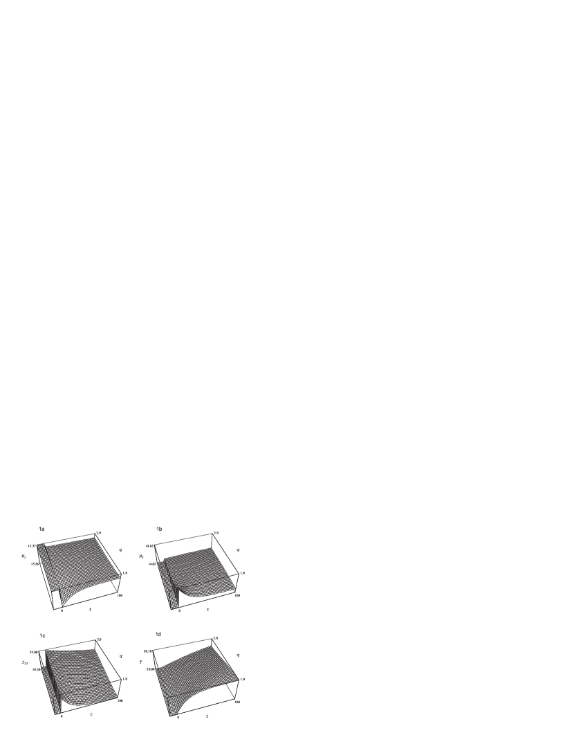
Figure 1: Plot (in arbitrary units) of time evolution of $N_{{}_{1}}$ (1a), $N_{{}_{2}}$ (1b), $I_{{}_{12}}$ (1c) and $T$ (1d) v.s. $q$, after injection, at $t=0$, of a flash of photons obeying to the $q$-Bose statistics.

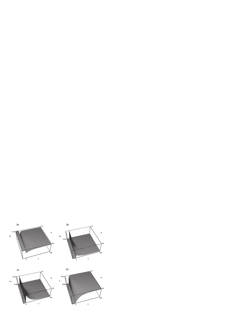
Figure 2: Plot (in arbitrary units) of time evolution of $N_{{}_{1}}$ (2a), $N_{{}_{2}}$ (2b), $I_{{}_{12}}$ (2c) and $T$ (2d) v.s. $\kappa$, after injection, at $t=0$, of a flash of photons obeying to the $\kappa$-Bose statistics.

In the following, we consider a system of $N$ atoms with $n=2$ levels and monochromatic photons with frequency $\omega_{{}_{12}}$. The system is initially in the equilibrium configuration at temperature $T^{\ast}$. From condition $B_{{}_{12}}=0$ follows the distribution $I_{{}_{12}}^{\ast}$.

Two different simulation are take into account. In the first simulation, a flash of photons is injected at the time $t=0$, from an isotropic external source at temperature $T^{\prime}$. The relaxation of the system to the new equilibrium configuration is depicted v.s. time in the following figures 1 and 2, concerning the results of two different generalizations adopted for the photons and described in the Appendix B. They take into account for an asymptotic inverse power law decay of the distribution function $I_{{}_{12}}$ with respect to $\omega_{ij}$.
First we adopt the model proposed by Büyükkiliç et al. [27, 28]. The time evolution of the physical meaningful quantities $N_{{}_{1}}$, $N_{{}_{2}}$, $I_{{}_{12}}$ and $T$ v.s. the deformed parameter $q$ is depicted in figures (1a), (1b), (1c) and (1d), respectively.
Then, we adopt the model proposed by Kaniadakis [7]. The time evolution of the physical meaningful quantities $N_{{}_{1}}$, $N_{{}_{2}}$, $I_{{}_{12}}$ and $T$ v.s. the deformed parameter $\kappa$ is depicted in figure (2a), (2b), (2c) and (2d), respectively.

In the second simulation, a constant and isotropic external photon source is inserted at the time $t=0$. Again, both the $q$-deformation and the $\kappa$-deformation are considered. The time evolution of the same physical quantities $N_{{}_{1}}$, $N_{{}_{2}}$, $I_{{}_{12}}$ and $T$ v.s. the deformed parameter $q$ [figures (3a), (3b), (3c) and (3d)] and v.s. the deformed parameter $\kappa$ [figures (4a), (4b), (4c) and (4d)] are plotted.

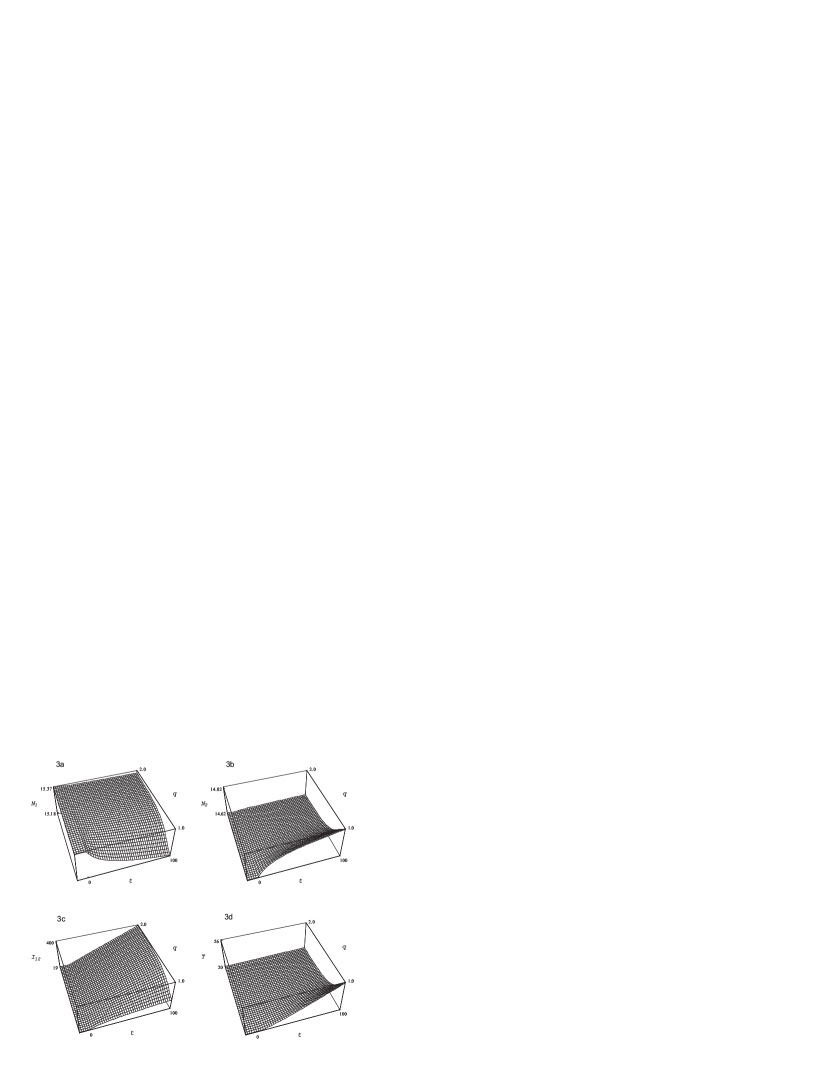
Figure 3: Plot (in arbitrary units) of time evolution of $N_{{}_{1}}$ (3a), $N_{{}_{2}}$ (3b), $I_{{}_{12}}$ (3c) and $T$ (3d) v.s. $q$, after the introduction, at $t=0$, of a constant photons source obeying to the $q$-Bose statistics.

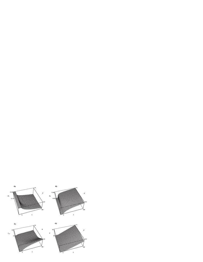
Figure 4: Plot (in arbitrary units) of time evolution of $N_{{}_{1}}$ (4a), $N_{{}_{2}}$ (4b), $I_{{}_{12}}$ (4c) and $T$ (4d) v.s. $\kappa$, after the introduction, at $t=0$, of a constant photons source obeying to the $\kappa$-Bose statistics.

A comparison between the $q$-deformed case and the $\kappa$-deformed case leads to the following considerations. With the respect to the classical case, the more the system is $\kappa$-deformed, the steeper the evolution is. On the contrary, the more the system is $q$-deformed the softer the evolution is.
We remark that this opposite behavior between the $q$-deformed case and the $\kappa$-deformed case is a consequence of the choice $q>1$. Such a choice arises from the observation that, in the present problem, for values of $q<1$ a cut-off in the energy spectrum is required. (see Eq. (2.1) in the Appendix B).
Moreover, from the second simulation we observe that, as well-known for the non-deformed case, in presence of a constant pumping of photons, the two number densities reach asymptotically, as $t\to\infty$, to the same value. Such a feature is preserved also in the deformed cases but with a different time-scale.

8 Conclusions

In order to improve the knowledge of the generalized statistical mechanics and generalized kinetic theory, we have investigated, in the present paper, a system of atoms and photons obeying to a very general statistics. The kinetic equations has been obtained, in the extended Boltzmann picture, through the introduction of characteristic departure and arrival functions for atoms and photons. In the space homogeneous case we have studied the equilibrium configuration. Such equilibrium is given by a modified Planck’s law for the radiation and by a generalized distribution function for the atoms.
By means of Lyapounov’s theory we have studied on the stability of this unique equilibrium configuration which maximize the entropic functional of the system.

In the second part of this paper we have considered a homogeneous and isotropic case keeping the generalization for photons only. Atoms are treated as classical particles. Under suitable assumptions on the relaxation times of the various interaction processes, according to the zero-order Chapmann-Enskog approximation, we have obtained a close system of macroscopic equations for the unknown dynamical quantities: the number density of atoms $N_{{}_{\ell}}$ at energy $E_{{}_{\ell}}$, the temperature of the system $T$ and the intensity $I_{{}_{ij}}$ at frequency $\omega_{{}_{12}}$.
We have shown the results of some numerical simulations for a system with $n=2$ energy levels. In the first simulation the system, initially at equilibrium at the temperature $T^{\ast}$, is perturbed by a flash of photons injected by a external source at a different temperature $T^{\prime}$. The relaxation of the system to the new equilibrium state for the physically relevant quantities $N_{{}_{1}}$, $N_{{}_{2}}$, $T$ and $I_{{}_{12}}$ has been plotted. In the second simulation the system, initially at equilibrium at the temperature $T^{\ast}$, is disturbed by a constant source of photons. The time evolution of the same physically relevant quantities has been plotted.

Appendix A

For sake of completeness, we report in this Appendix on the classical kinetic equations for atoms and photons, as known in literature.
The distribution function of atoms $A_{\ell}$ obeys to the following system of Boltzmann equations

$$\frac{\partial\,f_{{}_{\ell}}}{\partial\,t}+{\mbox{\boldmath${v}$}}\cdot{\mbox{\boldmath${\nabla}$}}f_{{}_{\ell}}=J_{{}_{\ell}}({\mbox{\boldmath${v}$}})+{\widetilde{J}}_{{}_{\ell}}({\mbox{\boldmath${v}$}})\ ,$$ (1.1)

where in the right hand side of Eq. (1.1) $J_{{}_{\ell}}({\mbox{\boldmath${v}$}})$ and ${\widetilde{J}}_{{}_{\ell}}({\mbox{\boldmath${v}$}})$ describe the contribution due to the atom-atom interaction and the contribution due to the atom-photon interaction, respectively.
In detail, for elastic/inelastic interactions between atoms we have

$$\hskip 22.76219ptJ_{{}_{\ell}}({\mbox{\boldmath${v}$}})=\sum_{j}\sum_{i\leq j}J^{{}^{(1)}}_{{}_{ij\ell}}({\mbox{\boldmath${v}$}})+\sum_{j}\sum_{i\leq j}J^{{}^{(2)}}_{{}_{ij\ell}}({\mbox{\boldmath${v}$}})+\sum_{k}\sum_{j\geq\ell}J^{{}^{(3)}}_{{}_{jk\ell}}({\mbox{\boldmath${v}$}})+\sum_{k}\sum_{i\leq\ell}J^{{}^{(4)}}_{{}_{ik\ell}}({\mbox{\boldmath${v}$}})\ ,$$ (1.2)

with

$$\hskip 28.45274ptJ^{{}^{(1)}}_{{}_{ij\ell}}({\mbox{\boldmath${v}$}})=\int_{I\!\!R^{3}\times S^{2}}g\,\sigma_{{}_{\ell j}}^{{}^{\ell i}}(g,\,\zeta)\,\left[f_{{}_{\ell}}({\mbox{\boldmath${v}$}}^{+}_{{}_{ij}})\,f_{{}_{i}}({\mbox{\boldmath${w}$}}^{+}_{{}_{ij}})-f_{{}_{\ell}}({\mbox{\boldmath${v}$}})\,f_{{}_{j}}({\mbox{\boldmath${w}$}})\right]\,d{\mbox{\boldmath${w}$}}\,d{\mbox{\boldmath${\Omega}$}}^{\prime}\ ,$$ (1.3)

$$\hskip 28.45274ptJ^{{}^{(2)}}_{{}_{ij\ell}}({\mbox{\boldmath${v}$}})=\int_{I\!\!R^{3}\times S^{2}}g\,\sigma_{{}_{\ell i}}^{{}^{\ell j}}(g,\,\zeta)\left[f_{{}_{\ell}}({\mbox{\boldmath${v}$}}^{-}_{{}_{ij}})\,f_{{}_{j}}({\mbox{\boldmath${w}$}}^{-}_{{}_{ij}})-f_{{}_{\ell}}({\mbox{\boldmath${v}$}})\,f_{{}_{i}}({\mbox{\boldmath${w}$}})\right]\,d{\mbox{\boldmath${w}$}}\,d{\mbox{\boldmath${\Omega}$}}^{\prime}\ ,$$ (1.4)

$$\hskip 28.45274ptJ^{{}^{(3)}}_{{}_{jk\ell}}({\mbox{\boldmath${v}$}})=\int_{I\!\!R^{3}\times S^{2}}g\,\sigma_{{}_{k\ell}}^{{}^{kj}}(g,\,\zeta)\left[f_{{}_{j}}({\mbox{\boldmath${v}$}}^{-}_{{}_{\ell j}})\,f_{{}_{k}}({\mbox{\boldmath${w}$}}^{-}_{{}_{\ell j}})-f_{{}_{\ell}}({\mbox{\boldmath${v}$}})\,f_{{}_{k}}({\mbox{\boldmath${w}$}})\right]\,d{\mbox{\boldmath${w}$}}\,d{\mbox{\boldmath${\Omega}$}}^{\prime}\ ,$$ (1.5)

$$\hskip 28.45274ptJ^{{}^{(4)}}_{{}_{ik\ell}}({\mbox{\boldmath${v}$}})=\int_{I\!\!R^{3}\times S^{2}}g\,\sigma_{{}_{k\ell}}^{{}^{ki}}(g,\,\zeta)\left[f_{{}_{i}}({\mbox{\boldmath${v}$}}^{+}_{{}_{i\ell}})\,f_{{}_{k}}({\mbox{\boldmath${w}$}}^{+}_{{}_{i\ell}})-f_{{}_{\ell}}({\mbox{\boldmath${v}$}})\,f_{{}_{k}}({\mbox{\boldmath${w}$}})\right]\,d{\mbox{\boldmath${w}$}}\,d{\mbox{\boldmath${\Omega}$}}^{\prime}\ ,$$ (1.6)

where $\sigma_{{}_{\ell i}}^{{}^{\ell j}}$ and $\sigma_{{}_{\ell j}}^{{}^{\ell i}}$ are the cross sections for forward and backward reactions, describing elastic and inelastic interactions.
In Eq.s (1.3)-(1.6) we have

$${\mbox{\boldmath${v}$}}^{\pm}_{{}_{ij}}={1\over 2}\,({\mbox{\boldmath${v}$}}+{\mbox{\boldmath${w}$}}+g_{{}_{ij}}^{\pm}\,{\mbox{\boldmath${\Omega}$}}^{\prime})\ ,\hskip 28.45274pt{\mbox{\boldmath${w}$}}^{\pm}_{{}_{ij}}={1\over 2}\,({\mbox{\boldmath${v}$}}+{\mbox{\boldmath${w}$}}-g_{{}_{ij}}^{\pm}\,{\mbox{\boldmath${\Omega}$}}^{\prime})\ ,$$ (1.7)

$$g_{{}_{ij}}^{\pm}=\sqrt{g^{2}\pm{4\over m}\,(E_{{}_{j}}-E_{{}_{i}})}\ ,\hskip 22.76219ptg=|{\mbox{\boldmath${v}$}}-\mbox{\boldmath${w}$}|\ ,$$ (1.8)

$${\mbox{\boldmath${\Omega}$}}=\frac{1}{g}\,({\mbox{\boldmath${v}$}}-{\mbox{\boldmath${w}$}})\ ,\hskip 76.82243pt\cos\zeta={\mbox{\boldmath${\Omega}$}}\cdot{\mbox{\boldmath${\Omega}$}}^{\prime}\ ,$$ (1.9)

and the two-dimensional unit sphere $S^{2}$ is the domain of integration for the unit vector ${\mbox{\boldmath${\Omega}$}}^{\prime}$. The four contributions to $J_{{}_{\ell}}({\mbox{\boldmath${v}$}})$ correspond to the cases in which $A_{{}_{\ell}}$ plays the role, in the reaction scheme (1.1), of $A_{{}_{k}}$ in the r.h.s., $A_{{}_{k}}$ in the l.h.s., $A_{{}_{i}}$ and $A_{{}_{j}}$, respectively.
For gas-radiation interactions, one can write

$${\widetilde{J}}_{{}_{\ell}}({\mbox{\boldmath${v}$}})=\sum_{i>\ell}\int_{S^{2}}{\widehat{J}}_{{}_{\ell i}}({\mbox{\boldmath${v}$}},\,{\mbox{\boldmath${\Omega}$}})\,d{\mbox{\boldmath${\Omega}$}}-\sum_{i<\ell}\int_{S^{2}}{\widehat{J}}_{{}_{i\ell}}({\mbox{\boldmath${v}$}},\,{\mbox{\boldmath${\Omega}$}})\,d{\mbox{\boldmath${\Omega}$}}\ ,$$ (1.10)

where

$${\widehat{J}}_{{}_{i\ell}}({\mbox{\boldmath${v}$}},\,{\mbox{\boldmath${\Omega}$}})=f_{{}_{\ell}}({\mbox{\boldmath${v}$}})\,\left[\alpha_{{}_{i\ell}}+\beta_{{}_{i\ell}}\,I_{{}_{i\ell}}({\mbox{\boldmath${\Omega}$}})\right]-\beta_{{}_{i\ell}}\,f_{{}_{i}}({\mbox{\boldmath${v}$}})\,I_{{}_{i\ell}}({\mbox{\boldmath${\Omega}$}})\ .$$ (1.11)

By taking into account all the energy levels higher than $\ell$, the loss term is due to absorption, while the gain term is due to spontaneous and stimulated emission. The situation is reversed when we consider all the energy levels lower than $\ell$.
The kinetic equation for photons $p_{ij}$ with intensity $I_{{}_{ij}}$ reads [22]:

$$\frac{\partial\,I_{{}_{ij}}}{\partial\,t}+{\mbox{\boldmath${\Omega}$}}\cdot{\mbox{\boldmath${\nabla}$}}I_{{}_{ij}}=\omega_{{}_{ij}}\,{\widetilde{J}}_{{}_{ij}}({\mbox{\boldmath${\Omega}$}})\ ,$$ (1.12)

where

$${\widetilde{J}}_{{}_{ij}}({\mbox{\boldmath${\Omega}$}})=\int_{I\!\!R^{3}}{\widehat{J}}_{{}_{ij}}({\mbox{\boldmath${v}$}},\,{\mbox{\boldmath${\Omega}$}})\,d{\mbox{\boldmath${v}$}}\ .$$ (1.13)

The gain term is due to spontaneous and stimulated emission, while the loss term is due to absorption.

Appendix B

We describe briefly two models used in the numerical simulations. They take into account an inverse power law decay of the distribution function with respect to energy [1, 2, 3].

1) The first model that we consider has been proposed by Büyükkiliç et al. [27, 28]. Relevant applications to the blackbody problem can be found in [12, 13]. Preliminarily, we define the $q$-deformed exponential and logarithm

$$\exp_{{}_{q}}(x)=[1+(1-q)\,x]_{{}_{+}}^{1/(1-q)}\ ,$$ (2.1)

$$\ln_{{}_{q}}(x)={x^{1-q}-1\over 1-q}\ ,$$ (2.2)

where $[x]_{+}=x$ for $x\geq 0$ and $[x]_{+}=0$ for $x<0$. These $q$-deformed functions have been introduced in thermo-statistics for the first time in Ref. [29].
The characteristic functions $\Phi$ and $\Psi$ are given by [15]

$$\Phi(x)=\exp\left[\ln_{{}_{q}}(x)\right]\ ,$$ (2.3)

$$\Psi(x)=\exp\left[\ln_{{}_{q}}(x)-\ln_{{}_{q}}\left({x\over 1+x}\right)\right]\ ,$$ (2.4)

where $1\leq q<2$ and for $q=1$ the standard statistics is recovered. For bosons we observe that the condition $\Psi(+\infty)=+\infty$ does not hold.
The deformed Bose-Einstein distribution function is given by

$$I_{{}_{ij}}={\alpha_{{}_{ij}}\over\beta_{{}_{ij}}}\,\left[{1\over\exp_{{}_{q}}(-\omega_{{}_{ij}}/T)}-1\right]^{-1}\ .$$ (2.5)

2) The second model that we consider has been proposed by Kaniadakis [7]. Preliminarily we define the $\kappa$-deformed exponential and logarithm

$$\exp_{{}_{\{\kappa\}}}(x)=\left(\sqrt{1+\kappa^{2}\,x^{2}}+\kappa\,x\right)^{1/\kappa}\ ,$$ (2.6)

$$\ln_{{}_{\{\kappa\}}}(x)={x^{\kappa}-x^{-\kappa}\over 2\,\kappa}\ .$$ (2.7)

Remarkably the $\kappa$-exponential satisfy the property $\exp_{{}_{\{\kappa\}}}(x)\,\exp_{{}_{\{\kappa\}}}(-x)=1$.The characteristic functions $\Phi$ and $\Psi$ are given by [15]

$$\Phi(x)=\exp\left[\ln_{{}_{\{\kappa\}}}(x)\right]\ ,$$ (2.8)

$$\Psi(x)=\exp\left[\ln_{{}_{\{\kappa\}}}(x)-\ln_{{}_{\{\kappa\}}}\left({x\over 1+x}\right)\right]\ ,$$ (2.9)

where $0\leq|k|<1$ and for $\kappa=0$ the standard statistics is recovered. In the case of bosons, the condition for $\Phi(+\infty)=+\infty$ is fulfilled as well. The deformed Bose-Einstein distribution function is given by

$$I_{{}_{ij}}={\alpha_{{}_{ij}}\over\beta_{{}_{ij}}}\,\left[\exp_{{}_{\{\kappa\}}}\left(\frac{\omega_{{}_{ij}}}{T}\right)-1\right]^{-1}\ .$$ (2.10)

References

References

• [1] Abe S 2001 Nonextensive Statistical Mechanics and its Applications, Okamoto Y editors, (Springer).
• [2] Special issue of Physica A 305, Nos. 1/2 (2002), Kaniadakis G, Lissia M and Rapisarda A editors.
• [3] Special issue of Physica A, (2004) Kaniadakis G and Lissia M editors; in press.
• [4] Kaniadakis G, Lavagno A and Quarati P 1996 Phys. Lett. B 369, 308.
• [5] Kaniadakis G, Lavagno A, Lissia M and Quarati P 1999 Proc. VII Workshop on Perspectives on Theoretical Nuclear Physics, 293, Fabrocini A, Pisent G and Rosati S editors.
• [6] Tsallis C, Barreto F C S and Loh E D 1995 Phys. Rev. E 52, 1447.
• [7] Kaniadakis G 2002 Phys. Rev. E 66, 056125.
• [8] Hsu R R and Lee C R 1993 Phys. Lett. A 180, 314.
• [9] Rego-Monteiro M, Roditi I and Rodrigues L M C S 1994 Phys. Lett A 188, 11.
• [10] Rego-Monteiro M, Rodrigues L M C S and Wulck S 1996 Phys. Rev. Lett. 76, 1098.
• [11] Alcaraz F C, Droz M, Henkel M and Rittenberg V 1994 Ann. Phys. 230, 250.
• [12] Wang Q A and Le Mehaute A 1998 Phys. Lett. A 242, 301.
• [13] Wang Q A, Nivanen L and Le Mehaute A 1998 Physica A 260, 490.
• [14] Rossani A and Kaniadakis G 2000 Physica A 277, 349.
• [15] Rossani A and Scarfone A M 2003 Physica B 334, 292.
• [16] Rossani A 2003 Physica A 305, 323.
• [17] Rossani A, Spiga G and Monaco R 1997 Mech. Res. Comm. 24, 237.
• [18] Riganti R and Rossani A 1998 Appl. Math. Comm. 96, 47.
• [19] Rossani A and Spiga G 1998 Transp. Th. and Stat. Phys. 27, 273.
• [20] Rossani A and Spiga G 1997 Rend. del Circ. Mat. di Palermo 57, 439.
• [21] Oxenius J 1986 Kinetic Theory of Atoms and Photons (Berlin: Springer-Verlag).
• [22] Pomraning G C 1973 The Equation of Radiation Gasdynamics (Oxford: Pergamon Press).
• [23] Ühling E A and Uhlenbeck G E 1933 Phys. Rev. ${43}$,552.
• [24] Liboff R L 1990 Kinetic Theory, (London: Prentice-Hall).
• [25] Chapman S and Cowling T G 1970 The Mathematical Theory of Non-Uniform Gases, (Cambridge: Cambridge University Press).
• [26] Yeremin E N 1986 Fundamentals of Chemical Thermodynamics (Moscow: Mir Publishers).
• [27] Büyükkiliç F and Demirhan D 1993 Phys. Lett. A ${181}$, 24.
• [28] Büyükkiliç F, Demirhan D and Güleç A 1995 Phys. Lett. A ${197}$, 209.
• [29] Tsallis C 1988 J. Stat. Phys. ${52}$, 479.