Phase Diagram and Critical Behavior of the Spin-1 Baxter-Wu Model with a Crystal Field

Abstract

The phase diagram and critical behavior of the spin-1 Baxter-Wu model with a crystal field in two dimensions is explored by renormalization group, conventional finite-size scaling and conformal invariance techniques. We found that the phase diagram of this model is qualitatively the same as that of the dilute 4-states Potts model, presenting a multi-critical point for a finite value of the crystal field, in disagreement with previous work based on finite-size calculations. However, our results indicate that the critical exponents vary continuously along the second-order transition line, differently from the expected behavior of the dilute 4-states Potts model.

I Introduction

The Ising model ons was the first non-trivial model exactly solvable in two dimensions which exhibits spontaneous symmetry breaking. It became the most popular ferromagnetic model in statistical mechanics and even today is the object of several studies in other contexts like random systems.priv The dynamics of the Ising model is described by the Hamiltonian

$$H_{I}=-J\sum_{<i,j>}s_{i}s_{j},$$ (1)

where the sum is over all nearest neighbors and the classical spin variables $s_{i}=\pm 1$ are attached at each site $i$ of the lattice. In middle 60’s, Blume and Capel s1mf proposed an extension of the Hamiltonian (1) to study first-order magnetic phase transitions. Their Hamiltonian is given by

$$H_{BC}=-J\sum_{<i,j>}s_{i}s_{j}+\Delta\sum_{i}s_{i}^{2},$$ (2)

where $\Delta$ plays the role of a crystal field and in this case the variables $s_{i}$ are classical spin-1 variables taking the values $s_{i}=-1,0,1$.

It is well established that for dimensions $d\geq 2$ the Blume-Capel model (Eq. (2)) presents a phase diagram with ordered ferromagnetic and disordered paramagnetic phases separated by a transition line which changes from a second-order character (Ising type) to a first-order one at a tricritical point (see Ref. new, and references there in). More specifically, in two dimensions, the machinery coming from conformal invariance ci1 ; ci2 indicates that at this multi-critical point the long-range fluctuations are governed by a conformal field theory with central charge $c=7/10$.new ; s1c.7 ; drugo In this case, all the critical exponents and the whole operator content of the model were obtained drugo (see also Ref. new, ). The generalization to higher spin $S$ of this model has also been studied.new ; srg ; s1.5mk ; s1.5mf ; plandau0 In particular, results of mean field theory,s1.5mf conformal invariance,new and Monte Carlo simulations plandau0 predict different phase diagrams for integer or half-odd-integer spins, in contradiction with results based on real space renormalization groups.srg ; s1.5mk Recently, the universality at a double critical endpoint in the two-dimensional spin-3/2 Blume-Capel model has been analyzed and it was shown that it belongs indeed to the same universality class as the critical line.plandau

Another simple model exactly solvable in two dimensions exhibiting spontaneous symmetry breaking is the Baxter-Wu model.bw ; ax1 ; ax2 This model is defined on a triangular lattice by the three-spin interaction Hamiltonian

$$H_{BW}=-J\sum_{<ijk>}s_{i}s_{j}s_{k},$$ (3)

where the sum extends over all elementary triangles of the lattice and $s_{i}=\pm 1$ are Ising variables located at the sites. This model is self-dual merlini with the same critical temperature as that of the Ising model on a square lattice. The critical behavior of the Baxter-Wu model is governed by a conformal field theory with central charge $c=1$, ax1 ; ax2 and its leading exponents bw ; ax1 ; ax2 $\alpha=2/3$, $\nu=2/3$ and $\eta=1/4$ are the same as those of the 4-states Potts model. dwbaxter

In analogy with the Blume-Capel model, in this paper we consider the Baxter-Wu model in the presence of a crystal field. The Hamiltonian of the spin-1 Baxter-Wu model with a crystal field is given by

$$H=-J\sum_{<ijk>}s_{i}s_{j}s_{k}+\Delta\sum_{i}s_{i}^{2},$$ (4)

where the classical spin variables $s_{i}$, defined in a triangular lattice, take the values $s_{i}=-1,0,1$. Note that when $\Delta\rightarrow-\infty$ only the configurations with $s_{i}=\pm 1$ are allowed, and we recover the pure Baxter-Wu model.

Since we have in the Baxter-Wu model with a crystal field the same kind of competition between the ordered ($\langle s\rangle\neq 0$) and the disordered phases ($\langle s\rangle=0$) (which is mediated by the crystal field) as in the Blume-Capel model, we may expect for both models a similar phase diagram, but with different critical behavior. This kind of competition also appears in the dilute $q$-states Potts model.nis It is well known that the Baxter-Wu model and the 4-states Potts model have the same critical exponents (see for example Ref. 14). Since the dilution in the 4-states Potts model has the same effect as the crystal field in the Baxter-Wu model, we may expect the critical behavior of both models to be the same. Some previous calculations of the phase diagram of both models have been reported in the literature. Nienhuis et al.,nis based on a renormalization-group study, indicate that for the dilute 4-states Potts model the phase diagram is similar as that of the Blume-Capel model, i.e., there is a transition line which changes from a second-order character to a first-order one at a multi-critical point. In this case, however, the critical behavior is governed by only one fixed point, giving along the second-order line the same exponents as that of the pure 4-states Potts model. On the other hand, Kinzel et al.,kda using finite-size methods, conjectured a different kind of phase diagram for the Baxter-Wu model in the presence of a crystal field. These authors interpreted the changes of the estimated thermal exponents $y_{t}$ along the transition line as a signal that a second-order transition should happen only for $\Delta\rightarrow-\infty$ (the pure Baxter-Wu model).

A careful study of the pure Baxter-Wu model has also been done by exploring its Bethe-ansatz solution.bw ; ax1 ; ax2 Using the consequences of conformal invariance, it has been shown ax1 ; ax2 that in the absence of dilution ($\Delta\rightarrow-\infty$) not only the leading critical exponents of the Baxter-Wu model and the 4-states Potts model are identical, but the whole operator content of the models coincides as well. Moreover, the masses of the field theory describing the thermal and magnetic perturbations of both models are also identical.ax2 Since the reported effects of the dilution in both systems are different, we decided in this paper to study the effect of dilution (or crystal field) in the Baxter-Wu model in two dimensions using the machinery of conformal invariance and renormalization group techniques.

This paper is organized as follows. In the next section we present the phase diagram obtained through the mean field renormalization group approach. In section III we present the transfer matrix of the model, the relations used in our finite-size studies, as well as the results for the phase diagram. We then close the paper in section IV with a summary and conclusions.

II Mean field renormalization group

The mean field renormalization group (MFRG)indekeu1 ; indekeu2 is a powerful phenomenological approach which can provide quite good results in the general study of critical phenomena.plarev It is based on the comparison of the order parameter for different finite lattices in the presence of symmetry breaking boundary conditions. For a finite cluster of $N$ spins, and considering the parameters of the Hamiltonian (4), one first computes the magnetization per spin $m_{N}(K,D,b)$, where $K=\beta J$, $D=\beta\Delta$ and $b$ is the boundary field, with $\beta=1/k_{B}T$ and $k_{B}$ the Boltzmann constant. As the boundary field is assumed to be very small one has

$$m_{N}(K,D,b)=f_{N}(K,D)b\leavevmode\nobreak\ .$$ (5)

In its simplest version, the MFRG considers two different clusters of $N^{\prime}<N$ spins and assumes that the magnetizations scale as

$$m_{N^{\prime}}(K^{\prime},D^{\prime},b^{\prime})=\ell^{d-y_{H}}m_{N}(K,D,b),$$ (6)

where $\ell=(N/N^{\prime})^{1/d}$ is the scaling factor, $d$ is the dimension of the lattice and $y_{H}$ the magnetic exponent. With the same relation for the boundary fields, namely

$$b^{\prime}=\ell^{d-y_{H}}b,$$ (7)

and taking into account expansion (5) one has

$$f_{N}(K,D)=f_{N^{\prime}}(K^{\prime},D^{\prime}),$$ (8)

which is independent of any scaling factor and is viewed as a renormalization recursion relation from which one gets fixed point solutions $K^{\prime}=K=K_{c}$ and estimates of correlation length critical exponents $\nu$ in the subset $D^{\prime}=D$.

Another version of the approach considers three different clusters of $N^{\prime\prime}$, $N^{\prime}$ and $N$ spins (in increasing order) together with the scaling (6) in such a way that one gets

$$f_{N^{\prime}}(K^{\prime},D^{\prime})b^{\prime}=\ell_{1}^{d-y_{H}}f_{N}(K,D)b,$$ (9)

$$f_{N^{\prime\prime}}(K^{\prime\prime},D^{\prime\prime})b^{\prime\prime}=\ell_{2}^{d-y_{H}}f_{N^{\prime}}(K^{\prime},D^{\prime})b^{\prime},$$ (10)

where the scaling factors are $\ell_{1}=(N/N^{\prime})^{1/d}$ and $\ell_{2}=(N^{\prime}/N^{\prime\prime})^{1/d}$. Imposing now that the boundary fields scale not as bulk magnetizations above, but as the surface field we obtain

$$b^{\prime}=\ell_{1}^{y_{hs}}b,\leavevmode\nobreak\ \leavevmode\nobreak\ \leavevmode\nobreak\ \leavevmode\nobreak\ \leavevmode\nobreak\ \leavevmode\nobreak\ b^{\prime\prime}=\ell_{2}^{y_{hs}}b^{\prime},$$ (11)

where $y_{hs}$ is the surface critical exponent. Eqs. (9)-(11) are now the renormalization recursion relation between the interaction parameters of the system. The exponent $d-y_{h}-y_{{hs}}$ is then determined self-consistently by imposing further that Eqs. (9) and (10) possess the same fixed point $K^{\prime\prime}=K^{\prime}=K=K_{c}$ for an invariant subset $D^{\prime\prime}=D^{\prime}=D$ (for further details and a comparison between these two approaches see Refs. indekeu2, and plarev, ). This version of the method is referred as surface bulk MFRG (SBMFRG).

Before applying the MFRG to the spin-1 Hamiltonian, defined by Eq. (4), it is worthwhile to measure the efficiency of the method by first treating the pure Baxter-Wu model (Eq. 3), where exact results are available. Since the model exhibits three different ferrimagnetic phases at low temperatures,comm it is supposed, at first sight, that the size of the finite blocks must be such that they will suitably accommodate them in an equivalent way throughout the lattice. These would dramatically restrict the size of the clusters. However, we note that by computing the sub-lattice magnetizations $m_{A}$, $m_{B}$ and $m_{C}$, by taking three different boundary fields $b_{A}$, $b_{B}$ and $b_{C}$, we obtain the same equations as by considering a homogeneous cluster where $m_{A}=m_{B}=m_{C}$ and $b_{A}=b_{B}=b_{C}$. This is not surprising, bearing in mind that the ferromagnetic phase is also coexisting with the other three ferrimagnetic ones at low temperatures. This means that, for practical purposes, we can consider only the ferromagnetic arrangement, allowing us to take blocks of any number of spins. This leads a huge simplification in the numerical acquisition of the functions $f_{N}(K)$. For this particular system, the best clusters are those which preserve the symmetry of the original lattice. They are made of symmetric triangles of $N=6,10,15,21,28$ spins. Although for $N=6$ we can obtain analytical expressions for $m_{6}(K,b)$ and $f_{6}(K)$, for $N\geq 10$ all the quantities have to be computed numerically. In Table 1, we present the critical temperature and critical exponent obtained according to the usual MFRG and also from the SBMFRG. It is also possible through the MFRG get an extrapolation. plarev Note that, for the present case, the extrapolated value is not so close to the exact result. This is, in fact,

Table 1: Results for the pure Baxter-Wu model according to the MFRG and SBMFRG approaches.

$N^{\prime}-N$	$K_{C}$	$\nu$
	MFRG
6-10	0.28667	2.78203
10-15	0.36565	1.89869
15-21	0.39335	1.55875
21-28	0.41077	1.37178
extrapolated	0.43768	0.69995
exact	0.44069	2/3
	SBMFRG
6-10-15	0.58138	1.06875
10-15-21	0.48090	1.08061
15-21-28	0.47832	0.99573

expected since the MFRG does not reproduce the exact value as the size of the lattices go to infinity.indekeu2 Although the SBMFRG does,indekeu2 the present clusters are still too small for us to get a reasonable extrapolation. However, as can be seen from Table 1, the temperatures are getting closer to the exact value as the size of the clusters increase. Note that, while the MFRG approaches the expected result from below, the SBMFRG does it from above. A common feature of the present renormalization group is still a worse estimate of the critical exponent when compared to the critical temperature. Nevertheless, in general, a reasonable picture of the criticality of the system is achieved from the approach.

We now proceed to the study of the spin-1 model with crystal field anisotropy. The same symmetry arguments also apply for this model. However, due to computer time, we were here limited to block sizes $N=6,10,15$. The phase diagram in the $\delta=\Delta/J$ versus $kT/J$ plane is depicted in Fig. 1 according to both procedures, as well

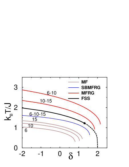
Figure 1: Phase diagram in the $\delta$ versus $kT/J$ plane for the spin-1 Baxter-Wu model in the presence of a crystal field. Continuum lines are second-order phase transitions and the dashed line is a first-order transition (see next section). The dot represent the multi-critical point. The results are according to the MFRG with two cluster, SBMFRG with three clusters, FSS (see next section) and MF approximation with one cluster. The sizes of the clusters used are also presented.

as from the finite-size scaling (FSS) procedure of the next section, and the usual mean field (MF) approximation. The latter approach, is obtained by assuming $m_{N}=b$ in Eq. (5), resulting in $f_{N}=1$. Except for the FSS, all the lines terminate at some point which is identified as the multi-critical point. The first-order transition lines are not possible to be obtained neither from the MFRG nor from the SBMFRG. Comparing with the FSS result, discussed in the next section, we can see that the MFRG overestimates the critical temperature while the surface bulk version underestimates it. This is just what happens in the pure case, as shown in Table 1, when compared to the exact critical value. ( nao entendi o q vc quer dizer… In all cases, the critical temperature of the spin-1/2 model is obtained in the limit $\delta\rightarrow-\infty$. pode tirar esta frase? Ja’ nao foi dita na introducao!) The estimate of the multi-critical point is given in Table 2. The SBMFRG and MFRG give critical exponents that vary along the second-order critical line. However, this fact, may be just an artifact of these aproaches, since there is only one renormalization recursion relation. plarev In the next section, we analize in the context of confomal invariance the possibility of the critical exponents vary along the second-order line.

Table 2: Position of the multi-critical point for the curves shown in Fig. 1.

$N^{\prime}-N$	$k_{B}T_{t}/J$	$\delta_{t}$
	MFRG
6-10	1.1816	2.1523
10-15	0.9330	1.8462
	SBMFRG
6-10-15	0.6408	1.5835
	MF
6	0.3133	0.8141
10	0.3539	1.0328
15	0.4513	1.1902
	FSS
3-6-9	1.2225	1.3089

III Finite-Size Scaling and Conformal Invariance

The row-to-row transfer matrix $\hat{T}$ of the Hamiltonian (4) in a triangular lattice, with horizontal width $N$, has dimension $3^{N}\times 3^{N}$. Its coefficients $\langle s_{1}^{\prime},...,s_{N}^{\prime}|\hat{T}|s_{1},...,s_{N}\rangle$ are the Boltzmann weights generated by the spin configurations $\{s_{1},...,s_{N}\}$ and $\{s_{1}^{\prime},...,s_{N}^{\prime}\}$ of adjacent rows. If we consider periodic boundary condition in the horizontal direction, the transfer matrix can be written as

$$\langle s_{1},...,s_{N}|\hat{T}|s_{1}^{\prime},...,s_{N}^{\prime}\rangle=$$

$$\prod_{j=1}^{N}\exp\left[t^{-1}s_{i+1}s_{i}^{\prime}(s_{i}+s_{i+1}^{\prime})-\delta t^{-1}s_{i}^{2}\right],$$ (12)

with $t=k_{B}T/J$ ($k_{B}$ is the Boltzmann constant) and $\delta=D/J$.

The finite-size behavior of the eigenvalues of $\hat{T}$ $(\Lambda_{0}(N)>\Lambda_{1}(N),...)$ can be used to determine the critical line and the critical exponents.ci1 ; ci2 ; fss The critical line $(t_{c}(\delta))$ is evaluated by extrapolating to the bulk limit ($N\rightarrow\infty$) the sequences $t_{c}(\delta,N)$ obtained by solving

$$G_{N}(t_{c})N=G_{N+3}(t_{c})(N+3),\leavevmode\nobreak\ \leavevmode\nobreak\ N=3,6,...$$ (13)

where $G_{N}(t_{c})$ is the mass gap of $H=-\ln\hat{T}$ and is given by

$$G_{N}(t_{c})=\ln\left(\frac{\Lambda_{0}(N)}{\Lambda_{1}(N)}\right).$$

The multi-critical points are obtained using a heuristic method, which has already been proved to be effective.new ; tripoint In this case we have to solve simultaneously (13) for three different lattice sizes

$$G_{N}(t_{c})N=G_{N+3}(t_{c})(N+3)=$$

$$G_{N+6}(t_{c})(N+6),\leavevmode\nobreak\ \leavevmode\nobreak\ N=3,6,...$$ (14)

In Eqs. (13) and (14) we restricted the possible finite strip widths to multiples of 3 in order to preserve the invariance of the Hamiltonian (4) under the reversal of all spins on any two sub-lattices.

As usual, we expect the model to be conformally invariant in the region of continuous phase transition. This invariance allows us to infer the critical properties from the finite-size corrections of the eigenspectrum at $t_{c}$.ci1 ; ci2 The conformal anomaly $c$, which labels the universality class of critical behavior, can be calculated from the large-$N$ behavior of the ground-state energy of $H=-\ln\hat{T}$ci2

$$\frac{\ln\Lambda_{0}(N)}{N}=\epsilon_{\infty}+\frac{\pi cv_{s}}{6N^{2}}+o(N^{-2}),$$ (15)

where $\epsilon_{\infty}$ is the the ground-state energy per site in the bulk limit and $v_{s}=\sqrt{3}/2$ is the sound velocity. The scaling dimensions of operators governing the critical fluctuations (related to the critical exponents) are evaluated from the finite-$N$ corrections of the excited states. For each primary operator, with dimension $x_{\phi}$, in the operator algebra of the system, there exists an infinite tower of eigenstates of $H=-\ln\hat{T}$ whose energy $\ln(\Lambda_{m,m^{\prime}}^{\phi})$ and momentum $P^{\phi}_{m,m^{\prime}}$ are given by ci1

$$\frac{\ln\Lambda_{m,m^{\prime}}^{\phi}(N)}{N} = \frac{\ln\Lambda_{0}(N)}{N}-\frac{2\pi v_{s}}{N^{2}}(x_{\phi}+m+m^{\prime})$$

$$P_{m,m^{\prime}}^{\phi} = \frac{2\pi}{N}(s_{\phi}+m-m^{\prime}),$$ (16)

where $m,m^{\prime}=0,1,\dots$.

A finite-size estimate for the first-order transition line can be obtained by the same procedure done as in a recent work.new At the first-order line of the Baxter-Wu model with a crystal field, we have the coexistence of five phases, one ordered ferromagnetically, three ordered ferrimagnetically and a disordered one. Consequently, for a given lattice size $N$ we calculate the points where the gap corresponding to the fifth eigenvalue has a minimum. The extrapolation $N\rightarrow\infty$ of these points give us an estimate for the first-order transition line.

In the numerical diagonalization of (12) we used the Lanczos method for non-Hermitian matrices.lanc We also considered the translational symmetry to block-diagonalize the transfer matrix.

In Fig. 1 we show the second-order transition line (continuum line), obtained by solving Eq. (13) for lattice sizes $N=6$. As we can see in this figure the second-order transition line also occur for finite values of the crystal field ($\delta\neq-\infty)$, differently of the previous results of Kinzel et al.,kda where it was conjectured the appearance of the second-order transition only at $\delta\rightarrow-\infty$. For the pure Baxter-Wu model ($\delta\rightarrow-\infty$) we obtained $t_{c}^{-1}=0.4408842$ for $N=6$ in Eq. (13), which differs only $0.04\%$ of the exact value $t_{c}^{-1}=\frac{\ln(\sqrt{2}+1)}{2}=0.440686...$ . For this reason, it is a very good approximation to consider $t_{c}(\delta)=t_{c}^{6,9}(\delta)$.

For the sake of clarity, we present in Table 3 the finite-size sequences obtained by solving Eq. (13) for lattice sizes $N=3$ and $N=6$. As we can see from this table the convergence of $t_{c}$ are better for $\delta>0$, so we expect that the estimates of $t_{c}^{(6,9)}(\delta)$ are better than the corresponding ones in the region $\delta<0$. The fast convergence with $N$ indicates that the corrections to finite-size are probably given by a power law, like in the pure Baxter-Wu model. In this last case the corrections are controlled by an operator with dimension $w=4$.ax1

Table 3: Finite-size data $t_{c}^{N,N+3}$ given by (13) for the critical temperature $t_{c}$ for some values of $\delta$.

N	-10	-1	1	1.25	1.3
3	2.246498	1.843818	1.358399	1.251121	1.226940
6	2.256769	1.849705	1.360144	1.251529	1.227005

We have also solved Eq. (14) for $N=3$, which gives us an estimate for the multi-critical point. In this case we do not have points to extrapolate, but we believe the estimate of the multi-critical point, the last point in the continuum line in Fig. 1, is not far from the extrapolated one. Our estimate for this point is $t_{t}=1.2225$ and $\delta_{t}=1.3089$.

We determined the first order line minimizing the gap related with the fifth eigenvalue, as discussed before. The dashed line shown in Fig. 1 was obtained in this procedure considering $N=9$. As we can see in this figure, the first-order transition line finishes at the multi-critical point.

In the critical regions of the phase transition line (continuum curve) the conformal anomaly and the scaling dimensions can be calculated exploring the conformal invariance relations (15) and (16). From Eq. (15) a possible way to extract $c$ is by extrapolating the sequence

$$c^{N,N+3}=\frac{12}{\sqrt{3}\pi}\left(\frac{\ln\Lambda_{1,0}(N+3)}{N+3}-\frac{\ln\Lambda_{1,0}(N)}{N}\right)\times$$

$$\left(\frac{1}{(N+3)^{2}}-\frac{1}{N^{2}}\right)^{-1},$$ (17)

calculated at $t_{c}(\delta)$. In Eq. (17) $\Lambda_{n,p}(N)$ means the $n$th eigenvalue of (12) with size $N$ in the sector with momentum $p$. Examples of such sequences for the Baxter-Wu model with a crystal field are shown in Table 4. The extrapolated values of $c^{\infty}$ can be obtained from the $N$-large behavior of $c^{N,N+3}(\delta)$, given by

$$c^{N,N+3}(\delta)=c^{\infty}-a\left(N^{-w}+(N+3)^{-w}\right)\times$$

$$\left(N^{-2}+(N+3)^{-2}\right)^{-1},$$ (18)

where $a$ is a constant and $w$ the dominant dimension associated to the operator governing the finite-size corrections. We determine $c^{\infty}$ assuming Eq. (18) exact for $N=3$ and $N=6$ with $w$ given by the pure Baxter-Wu model, i.e. $w=4$.ax1 We see from Table 4 that the conformal anomaly is $c=1$ along the critical line, and apparently even at the multi-critical point. This scenario is quite different from that of the Blume-Capel model, where the conformal anomaly changes abruptly from $c=1/2$ at the critical line to $c=7/10$ at the tricritical point (see Ref. 5), but its qualitatively similar as that of the dilute 4-states Potts model,nis where along of the critical line the critical exponents as well the conformal anomaly do not change. Since we do not have a precise estimate for the multi-critical point, we have also calculated $c^{N,N+3}$ for several values of $t_{c}(\delta)$ between $1.2<t_{c}(\delta)<1.4$. We have not seen any abrupt change of the conformal anomaly, like in the Blume-Capel model.new

Table 4: Finite-size estimates $c^{N,N+3}$, given by (17), for the conformal anomaly is shown for some values of $\delta$. The extrapolated results obtained by (18) is also shown.

N	-10	-1	1	1.25	1.3089
3	0.938546	0.941169	0.954322	0.955674	0.955047
6	0.986393	0.986829	0.986656	0.979694	0.975435
$\infty$	1.006	1.005	0.999	0.989	0.984

From Eq. (16) the scaling dimensions $x(n,p)$ related to the $n$th ($n=1,2,\ldots$) energy in the sector with momentum $p$ can be obtained by extrapolating the sequence

$$x^{N}(n,p)=\frac{N}{\pi\sqrt{3}}\ln\left(\frac{\Lambda_{1,0}(N)}{\Lambda_{n,p}(N)}\right).$$ (19)

Table 5: Finite-size scaling dimensions $x^{N}(1,0)$ and $x^{N}(2,0)$ given by (19) for some values of $\delta$.

		N=9	N=6	N=3
	$\delta$=-10	0.1236	0.1236	0.1195
	$\delta$=-1	0.1223	0.1223	0.1184
$x^{N}(1,0)$	$\delta$=1	0.1113	0.1113	0.1093
	$\delta$=1.25	0.1048	0.1048	0.1043
	$\delta$=1.3089	0.1026	0.1026	0.1026
	$\delta$=-10	0.5059	0.5147	0.6057
	$\delta$=-1	0.4897	0.4976	0.5756
$x^{N}(2,0)$	$\delta$=1	0.3644	0.3762	0.4163
	$\delta$=1.25	0.3023	0.3207	0.3613
	$\delta$=1.3089	0.2829	0.3037	0.3456

In Table 5 we show the dimensions $x^{N}(1,0)$ and $x^{N}(2,0)$ for the Baxter-Wu model with a crystal field. Note that $x^{9}(1,0)=x^{6}(1,0)$ due the Eq. 13 and the fact we choose $t_{c}(\delta)=t_{c}^{6,9}(\delta)$. In the tricritical point the three entries $x^{N}(1,0)$ are same due Eq. 14. For $\delta\rightarrow-\infty$ (the pure Baxter-Wu model) the scaling dimensions $x^{9}(1,0)$ and $x^{9}(2,0)$ differ only $1\%$ from the leading dimensions $x^{9}(1,0)=\frac{1}{8}$ and $x^{9}(2,0)=\frac{1}{2}$ of the pure Baxter-Wu model. As the estimate of the critical line is better in the region $\delta>0$ and the eigenvalues converge faster with the size of the lattice in this region, we believe that our estimates for the scaling dimensions are better in the region $\delta>0$ than the corresponding ones for $\delta<0$, i.e., the estimates $x^{9}(1,0)$ and $x^{9}(2,0)$ must differ by less than $1\%$ from the extrapolated values for $\delta>0$. Note that when we increase the crystal field $\delta$ these values change continuously up to $x^{9}(1,0)\sim 0.10$ and $x^{9}(2,0)\sim 0.28$ at the multi-critical point. This scenario is quite different from that of the Blume-Capel model, which is not a surprise since both models are in different universality classes of critical behavior. However it is also distinct from the scenario of the dilute 4-states Potts model, where the scaling dimensions along the critical line are believed to be the same as that of the pure 4-states Potts model. If the dilution had the same role in both models, we should expect for the dilute 4-states Potts a continuous line of fixed point, however this was not found.nis

IV Summary and Conclusion

In this paper we have calculated the phase diagram and critical properties of the spin-1 Baxter-Wu model in the presence of a crystal field. Our results, based on renormalization group, finite-size scaling and conformal invariance, show a second-order transition line separated from a first-order transition line by a multi-critical point. This scenario is in disagreement with that of a previous paper by Kinzel et al., kda where the second-order transition line appears only in the limiting case $\Delta\rightarrow-\infty$. The critical behavior was determined by renormalization group and conformal invariance. Despite the phenomenological renormalization group be not so conclusive regarding the critical exponents, the conformal invariance results indicate that along the critical line, and even at the multi-critical point,the conformal anomaly is the same as that of the Baxter-Wu model or the 4-states Potts model, i.e., $c=1$, in agreement with the scenario expected for the dilute 4-states Potts model. However, our results indicate that the scaling dimensions vary continuously with the crystal field. This is an unexpected behavior since the reported results for the dilute 4-states Potts model indicate a constancy of the scaling dimensions along the phase transition line,nis and it is expected that both models belong to the same universality class of critical behavior. This result implies that either contrary to what occurs with thermal and magnetic perturbations the effect of dilution is distinct in the Baxter-Wu and in the 4-states Potts models, or the scenario based in renormalization group for the dilute 4-states Potts model is wrong. It would be interesting to verify our results using different numerical techniques, like Monte Carlo methods. In fact, a Monte Carlo simulation for the case $\delta=0$ has already been done and different exponents as those of the pure Baxter-Wu model have been achieved.moraes Extensive Monte Carlo simulations for $\delta\neq 0$ are in progress and will be present elsewhere. moraes2

Acknowledgments

JCX would like to acknowledge profitable discussions with M. J. Martins and J. R. G. de Mendonça. He is also indebted to F. C. Alcaraz for suggestions and discussions in part of this work. This work was supported by FAPESP (Grants 00/02802-7 and 01/00719-8) (JCX), FAPEMIG (MLMC and JAP), CNPq (JAP) and CAPES (MLMC).

References

- (1) L. Onsager, Phys. Rev. 65, 117 (1944).
- (2) M. P. Nightingale, in Finite Size Scaling and Numerical Simulations in Statistical Systems, edited by V. Privman (World Scientific, Singapore, 1990).
- (3) M. Blume, Phys. Rev. 141, 517 (1966); H. W. Capel, Physica 32, 966 (1966).
- (4) J. C. Xavier, F. C. Alcaraz, D. P. Lara , and J. A. Plascak, Phys. Rev. B 57, 11575 (1998).
- (5) J. L. Cardy, Phase Transitions and Critical Phenomena vol 11, edited by C. Domb and J. L. Lebowitz (Academic, New York, 1987).
- (6) H. W. J. Blöte, J. L. Cardy and M. P. Nightingale, Phys. Rev. Lett. 56, 742 (1986); I. Affleck, ibid. 56, 746 (1986).
- (7) F. C. Alcaraz, J. R. D. de Felício , R. Köberle and J. F. Stilck, Phys. Rev. B 32, 7469 (1985).
- (8) D. B. Balbão and J. R. Drugowich de Felício, J. Phys. A: Math. Gen. 20, L207 (1987); G. v. Gehlen, ibid. 24, 5371 (1990).
- (9) S. M. de Oliveira, P. M. C. de Oliveira and F. C. de Sá Barreto, J. Stat. Phys. 78, 1619 (1995).
- (10) A. Bakchich, A. Bassir and A. Benyoussef, Physica A 195, 188 (1993).
- (11) J. A. Plascak, J. G. Moreira and F. C. Sá Barreto, Phys. Lett. A 173, 360 (1993).
- (12) J. A. Plascak and D. P. Landau, Computer Simulation Studies in Condensed Matter Physics XIII, D. P. Landau, S. P. Lewis and H.-B. Shuttler (eds) (Springer, Berlin, Heidelberg 2000).
- (13) J. A. Plascak and D. P. Landau, Phys. Rev. E 67, R015103 (2003).
- (14) R. J. Baxter and F. Y. Wu, Phys. Rev. Lett. 31, 1294 (1973); R. J. Baxter and F. Y. Wu, Aust. J. Phys. 27, 357 (1974); R. J. Baxter, Aust. J. Phys. 27, 369 (1974).
- (15) F. C. Alcaraz and J. C. Xavier, J. Phys. A: Math. Gen. 30, L203 (1997).
- (16) F. C. Alcaraz and J. C. Xavier, J. Phys. A: Math. Gen., 32, 2041-2060 (1999).
- (17) D. Merlini and C. Gruber, J. Math. Phys. 13, 1814 (1972); D. W. Wood and H. P. Griffiths, J. Phys. C 5, L253 (1972).
- (18) E. Domany and E. K. Riedel, J. App. Phys. 49, 1315 (1978); F. Y. Wu, Rev. Mod. Phys. 54, 235 (1982); R. J. Baxter, Exactly Solved Models in Statistical Mechanics (Academic, New York, 1982).
- (19) B. Nienhuis, A. N. Berker, E. K. Riedel and M. Schick, Phys. Rev. Lett. 43, 737 (1979).
- (20) W. Kinzel, E. Domany and A. Aharony, J. Phys. A: Math. Gen. 14, L417 (1981).
- (21) J. O. Indekeu, A. Maritan and A. L. Stella, J. Phys. A, L291 (1982).
- (22) J. O. Indekeu, A. Maritan and A. L. Stella, Phys. Rev. B 35, 305 (1987).
- (23) J. A. Plascak, W. Figueiredo and B. C. S. Grandi, Braz. J. Phys. 29, 3 (1999).
- (24) Let , , and be the density of magnetization of the three sub-lattices. The three ferrimagnetic phases correspond to a phase where the magnetization has the following values , , and . There is also a ferromagnetic phase at low temperature given by .
- (25) M. N. Barber, Phase Transitions and Critical Phenomena vol 8, edited by C. Domb and J. L. Lebowitz (Academic, New York, 1983).
- (26) M. E. Fisher and N. Berker, Phys. Rev. 26, 2707 (1982); P. A. Rikvold, W. Kinzel, J. D. Gunton and K. Kaski Phys. Rev. B 28, 2686 (1983); H. J. Hermann, Phys. Lett. A 100, 156 (1984); A. L. Malvezzi, Braz. J. Phys. 24, 508 (1994).
- (27) G. H. Golub and C. F. van Loan, Matrix Computations, 3rd ed. (The Johns Hopkins University Press, Baltimore, 1996).
- (28) M. L. M. Costa and J. A. Plascak, to appear in Braz. J. Phys.
- (29) M. L. M. Costa and J. A. Plascak, unpublished.