Elastic scattering losses in the four-wave mixing of Bose Einstein Condensates

Abstract

We introduce a classical stochastic field method that accounts for the quantum fluctuations responsible for spontaneous initiation of various atom optics processes. We assume a delta-correlated Gaussian noise in all initially empty modes of atomic field. Its strength is determined by comparison with the analytical results for two colliding condensates in the low loss limit. Our method is applied to the atomic four wave mixing experiment performed at MIT [Vogels et. al., Phys. Rev. Lett. 89, 020401, (2002)], for the first time reproducing experimental data.

PACS numbers 03.75.Hh, 05.30.Jp

In recent years we observe a growing number of experiments in which the atomic Bose-Einstein condensate evolves in a nontrivial way. A whole new area of nonlinear atom optics was born. The most striking example of such a nonlinear process is the atomic four-wave mixing (4WM). In close analogy to its optical counterpart, atomic 4WM consists of generation of the new atomic beam in the nonlinear interaction of three overlapping matter waves. For the main part atomic 4WM is an example of a stimulated process. However, during this process there are also collisions between individual atoms that lead to a population of initially unoccupied atomic states. These processes have spontaneous initiation but by nature they are also examples of the four particle mixing. They amount to the elastic scattering losses from the coherently evolving condensates.

The standard tool used to describe dynamics of the condensate within mean field approximation is the celebrated Gross-Pitaevskii equation (GPE). As it stands, it is capable of describing stimulated processes but not the spontaneous ones. However, at least in some experiments  Vogels the elastic scattering losses may become significant. There are at least two theoretical attempts to estimate such losses during the collision of condensates. In the first one  Band the authors used momentum-dependent higher order correction to the nonlinear coupling constant in the GPE, introducing complex scattering length. In the second one  Yuro ; Keith ; Bach the field theoretical formulation was used. To make it effective, the authors approximate the second quantized hamiltonian by a quadratic form. Both methods give very similar results but are applicable only if the elastic scattering losses are merely a small correction.

It is the purpose of this Letter to formulate a general method of describing elastic scattering losses in the nonlinear atom optics processes. To this end we add to the GPE a classical gaussian noise, representing vacuum quantum fluctuations of the atomic field and an auxiliary field holding atoms scattered out from BEC. Such a technique has its roots in quantum optics.

Spontaneous optical processes have their origins in quantum fluctuations. The best known example is a process of superfluorescence  Vrehen . In this phenomenon a sample of atoms is prepared in the internal excited state. Spontaneously emitted photons create an avalanche of photon emissions. When the light field becomes strong, it is well described by a classical electromagnetic field. However the initiation has a quantal nature. This quantum initiation was successfully imitated by a classical noise  Haake . There are also general methods of mapping quantum fluctuations into stochastic term in the evolution equations of quantum optics (generalised P-representation methods) drumm .

In optics one can find numerous other processes initiated by spontaneous emission and eventually upon populating empty modes turning into stimulated processes; eg. spontaneous Raman scattering Raman , parametric down conversion paradown , etc. There are also similar examples in atomic and molecular physics molec . Our method is general and is capable of treating many of these processes. Here we demonstrate the method using the 4WM of coherent matter waves.

The first experiment demonstrating 4WM in a sodium Bose-Einstein condensate was performed at NIST Deng . This was followed by a theoretical and numerical treatment of the experiment  Trip ; Gold . In the experiment, a short time of free expansion of the condensate, after it was released from the magnetic trap, was followed by a set of two Bragg pulses Kozuma , which created moving wavepackets. These wavepackets, together with the remaining stationary condensate, due to nonlinear interaction and under phase matching conditions created a new momentum component in the 4WM process. The standard starting point for the description of atomic 4WM process is the Gross-Pitaevskii equation

$$i\hbar\partial_{t}\Psi(\vec{r},t) = \left(-\frac{\hbar^{2}\nabla^{2}}{2m}+V+gN|\Psi|^{2}\right)\Psi(\vec{r},t).$$ (1)

Here $N$ is the total number of atoms, $|\Psi|^{2}$ is proportional to the atomic number density and is normalized to one, $g=4\pi\hbar^{2}a/m$ is the nonlinear interaction strength, $m$ the atomic mass, $a$ is the scattering length and $V$ is a confining potential. A compact ground state wavefunction $\Psi(\vec{r},0)$ is created in harmonic trap potential $V$ and centered around $r=0$ with $\Psi(0,0)=\Psi_{m}$, the maximum value. Once this ground state is created, V is turned off. The development of $\Psi(\vec{r},t)$ is now described by Eq. (1) with $V=0$. Later on, a set of Bragg pulses is applied and parts of the condensate begin to move. We can define two timescales characterizing evolution of the condensate: a nonlinear interaction time $\tau_{{\rm NL}}=(gN|\Psi_{m}|^{2}/\hbar)^{-1}$ and a collision time $\tau_{{\rm col}}$. The latter is defined as a time it takes two wavepackets uniformly moving along $x$ to move apart (so they just touch and cease to overlap), $\tau_{{\rm col}}=2r_{{\rm TF}}/v$ where $r_{{\rm TF}}$ is the initial radius of the condensate in the $x$ direction (Thomas - Fermi approximation), and $v$ is the relative velocity. The ratio of these two timescales determines the output of the 4WM process.

The initial condition immediately after application of the Bragg pulses at $t_{1}$, can be approximated as being a composition of the BEC wavepackets, identical in shape to $\Psi(\vec{r},t_{1})$ (for more details see Trip ):

$$\Phi(\vec{r},t_{1}) = \Psi(\vec{r},t_{1})\sum_{i=1}^{3}f_{i}^{1/2}{\rm e}^{i\vec{P}_{i}\vec{r}/\hbar}.$$ (2)

Here $f_{i}=N_{i}/N$ is the fraction of atoms in the $i$-th wavepacket and $\sum_{i=1}^{3}f_{i}=1$. A new wavepacket with $\vec{P}_{4}=\vec{P}_{1}-\vec{P}_{2}+\vec{P}_{3}$ will build up, thanks to the nonlinear interactions accounted for by the last term in the Gross Pitaevskii equation (1). After a while, the fourth wavepacket will grow to the macroscopic level. Using the de Broglie relations: $\vec{k}_{i}=\vec{P}_{i}/\hbar$ and $\omega_{i}=\hbar k_{i}^{2}/2m$ we have:

$$\Phi(\vec{r},t) = \sum_{i=1}^{4}\Phi_{i}(\vec{r},t){\rm e}^{i(\vec{k}_{i}\vec{r}-\omega_{i}t)},$$ (3)

with initial conditions

$$\Phi_{i}(\vec{r},t_{1})=f_{i}^{1/2}\Psi(\vec{r},t_{1}),\,\,\,i=1,2,3; \Phi_{4}(\vec{r},t_{1})=0.$$

Variation of the $\Phi_{i}$ is assumed to be slow as compared to that of the exponential in equation (3). Four equations for this slow dependence are obtained from (1) and (3). We have, when $V$ is turned off Band :

$$\imath\hbar\partial_{t}\psi_{i} = -\frac{\hbar^{2}}{2m}\nabla^{2}\psi_{i}+gN(|\psi_{i}|^{2}+2\sum_{j\neq i}|\psi_{j}|^{2})\psi_{i}$$ (4)

$$+ 2gN\psi_{i+1}\psi_{i+2}^{*}\psi_{i+3}$$

where we use the convention in which all indices are taken modulo 4. To account for the elastically scattered atoms we introduce an additional component of the wavefunction $\psi_{B}$. It is this part of the wavefunction which will be initiated by the classical stochastic field. The stochastic field $\xi_{ij}(\vec{r},t)$ must be added to the equation of motion (4) to trigger the elastic scattering process of two particles from the condensate wavefunctions $\psi_{i}$ and $\psi_{j}$ to the background field $\psi_{B}$. It is a four particle process and it must be implemented for each pair of colliding wavefunctions $i,j$ in such a way that the total number of atoms in colliding waves + background field is still conserved. The resulting set of equations reads

$$(\imath\hbar\partial_{t}+\frac{\hbar^{2}}{2m}\nabla^{2})\psi_{i} = gN(|\psi_{i}|^{2}+2\sum_{j\neq i}|\psi_{j}|^{2}+2|\psi_{B}|^{2})\psi_{i}$$ (5)

$$+ gN\sum_{j\neq i}\psi_{j}^{*}\psi_{B}(\psi_{B}+\xi_{ij})$$

$$+ 2gN\psi_{i+1}\psi_{i+3}\psi_{i+2}^{*}$$

$$(\imath\hbar\partial_{t}+\frac{\hbar^{2}}{2m}\nabla^{2})\psi_{B} = +gN(|\psi_{B}|^{2}+2\sum_{i=1}^{4}|\psi_{i}|^{2})\psi_{B}$$ (6)

$$+ gN\sum_{i\neq j}\psi_{i}\psi_{j}(\psi_{B}+\xi_{ij})^{*}$$

For numerical calculations we assume that $\xi_{ij}(\vec{r},t)$ is a gaussian stochastic process with zero mean and the only nonvanishing second order correlation function equal to $\langle\xi_{ij}^{*}(\vec{r},t)\xi_{ij}(\vec{r}^{\prime},t^{\prime})\rangle=A_{ij}\delta_{\vec{r},\vec{r}^{\prime}}\delta_{t,t^{\prime}}$. Here Kronecker delta functions are assumed both in space and time since we refer to numerical simulations with spacial grid and discrete time steps. Notice that we assign different stochastic process to each pair of colliding wavepackets, anticipating dependence on parameters like relative velocity.

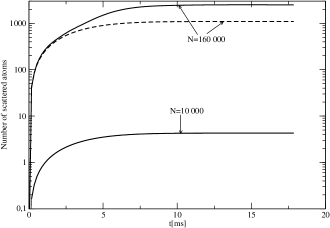
Figure 1: Number of elastically scattered atoms from the pair of counter-propagating condensate Gaussian wavefunctions, with relative velocity $1.75\,mm/s$, as a function of time. The lower curve corresponds to small number of scattered atoms ($N=10^{4}$ and gaussian width $\sigma=9.1\,\mu m$), when the bosonic stimulation does not occur. In this limit all three methods: complex scattering length calculation Band , field theory Bach , and our stochastic method give indistinguishable results. The upper pair of curves corresponds to higher number of atoms ($N=1.6\cdot 10^{5}$ and gaussian width $\sigma=15.8\,\mu m$) - dashed line was obtained using complex scattering length method and the solid line is a solution of eq.(8)

Equations (5-6) may be obtained from multiatom system hamiltonian upon using Bogoliubov decomposition of the atomic field operators into condensate parts and initially empty modes $\psi=\sum_{i=1}^{4}\psi_{i}+\psi_{B}$ in a way analogous to that presented in Bach . We do not however explicitly decompose $\psi_{B}$ into plane waves but obtain it’s Heisenberg equation of motion assuming only that it commutes with operators of macroscopically occupied modes $\psi_{i}$. Finally stochastic field is added to $\psi_{B}$ in the source terms for 4WM as shown above. These stochastic terms mimic vacuum quantum fluctuations leading to spontaneous elastic scattering loss. But as elastically scattered atoms reside in $\psi_{B}$ they may eventually get amplified via bosonic stimulation when population becomes significant. This is an outline of our stochastic method; details will be presented elsewhere Jachwed .

To fully determine equations (5-6) we need to specify the value of constants $A_{ij}$. Just as it has been done in the case of superfluorescence mentioned above, we can find $A_{ij}$ by the requirement that it reproduces known limiting analytic results  Bach . In reference  Bach the elastic scattering losses were computed analytically in perturbative regime for two colliding gaussian-shaped wave packets. Furthermore these wavepackets were assumed to evolve without losses and without spreading. The number of elastically scattered atoms as a function of time was found in the form

$$\mathcal{S}(t) = \left(\frac{Na}{\sigma}\right)^{2}\mathrm{Erf}\left(\frac{\sqrt{2}\hbar Q}{m\sigma}t\right),$$ (7)

where $\sigma$ is a width of the gaussian wave-packets and $Q$ is the wave vector corresponding to the absolute value of the momentum of each of the wave-packets in the center of mass frame. The same quantity might be calculated approximately under analogous assumptions using the stochastic classical noise. The equation for $\psi_{B}$ in this case reads

$$\imath\hbar\partial_{t}\psi_{B} = -\frac{\hbar^{2}}{2m}\nabla^{2}\psi_{B}+gN\left(|\psi_{B}|^{2}+2|\psi_{1}|^{2}+2|\psi_{2}|^{2}\right)\psi_{B}$$ (8)

$$+ 2gN\psi_{1}\psi_{2}(\psi_{B}+\xi_{12})^{*},$$

where $\psi_{1,2}$ are two counter-propagating gaussian wavefunctions. The approximations of Bach amounts in retaining on the right hand side of equation 8 only the last term. The approximate solution obtained this way gives the number of elastically scattered atoms as a function of time in the form

$$\mathcal{S}_{stoch}(t) = A_{12}\Delta t\frac{4\pi\hbar}{m(2Q)}\left(\frac{Na}{\sigma}\right)^{2}\mathrm{Erf}\left(\frac{\sqrt{2}\hbar Q}{m\sigma}t\right).$$ (9)

Comparing (7) with (9) we obtain $A_{12}=\frac{m(2Q)}{4\pi\hbar\Delta t}$. As we anticipated $A_{12}$ depends on the relative velocity of wavepackets $\psi_{1}$ and $\psi_{2}$, which in our case is equal $(2Q)$. Note that once $A_{ij}$’s are determined our numerical approach has no more adjustable parameters. In Fig. 1 we are comparing the solution of (7) with a numerical solution of full equation (8). Note the growing discrepancy between perturbative and non-perturbative results for larger losses. They result from bosonic enhancement present in the non-perturbative regime. We also stress that in the non-perturbative regime the stochastic noise is crucial at the early stage of evolution. It may even be dropped from equation (8) when Bose enhancement takes effect. This is why the strength of classical noise may be determined in the perturbative regime. Finally, we point out that some analogies regarding the break down of perturbative approach were found in the study of atom-molecule conversion within positive-P representation Olsen ; Poulsen .

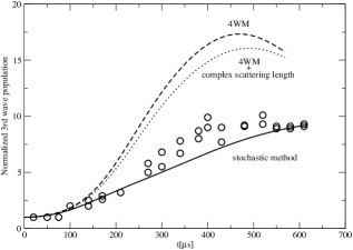
Figure 2: Population of the third wavepacket normalized to the initial seed population as a function of time (continuous line). Parameters used in the simulation correspond to experiment performed in the Ketterle group  Vogels . Total number of atoms equal to 5mln. Also shown: circles - experimentally measured values, and dashed and dot lines - solutions of the Gross-Pitaevskii equation with real and complex scattering length respectively.

With the equations (5-6) fully determined we turn our attention to the recent experiment from MIT  Vogels . This experiment, due to the large value of the ratio of collision to nonlinear timescales, had very large number of elastically scattered atoms. Experimental configuration consists of two initial wavepackets of equal strength ($\approx N/2$ atoms in each) and the third wavepacket of just a tiny fraction of N. Magnetic trap used to generate the Sodium condensate had frequencies of $80$, $80$ and $20$ Hz in axial direction, hence it has a shape of a cigar. Applied optical Bragg pulses to create moving wavepackets propagated approximately at the same angle of $\approx 0.5$ rad with respect to the long axis of the condensate corresponding to a relative velocity of $20$ mm/s. In two series of 4WM measurements chemical potential of the condensate was $2.2$ and $4.4$ kHz, which we identified as corresponding to $5$ and $30$ million atoms respectively. In Figure 2 we plot the population of the third wave-packet (the one that was initially seeded) as a function of time. The circles are the experimental data extracted from paper  Vogels . Several theoretical curves are plotted. The dashed line represents results neglecting all elastic scattering losses. The dotted line accounts for the losses by means of the complex scattering length Band . We see that neither of the curves reproduces experimental results. Our stochastic method gives the solid line which is much closer to the experimental data. It has been computed with the parameters of the experiment including the initial number of atoms infered from the paper as being equal to 5mln.

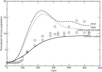
Figure 3: Population of the third wavepacket normalized to the initial seed population as a function of time (continuous line). Parameters used in the simulation correspond to experiment performed in the Ketterle group  Vogels . Total number of atoms equal to 30 mln. Also shown: circles - experimentally measured values, and dashed and dot lines - solutions of the Gross-Pitaevskii equation with real and complex scattering length respectively.

In Fig.3 similar comparison is made for larger sample of 30mln atoms. Again our results reproduce the experimental data very well. We feel that remaining discrepancy (our results seem to be consistently under experimental points) is due to indistinguishability of BEC and thermal atoms in the region of the momentum space occupied by BEC.

In conclusion: We have formulated the classical stochastic field method that accounts for the quantum fluctuations responsible for spontaneous initiation of various atom optics processes. For instance we can treat oscillations between atomic and molecular condensates triggered by optical or magnetic field effects  Olsen ; Poulsen . The method is then applied to the atomic 4WM. It gives for the first time excellent agreement with the recent MIT experiment, where the scattering losses where substantial.

We acknowledge stimulating discussions with Mariusz Gajda, Piotr Deuar and Keith Burnett. The authors would like to acknowledge support from KBN Grant 2P03 B4325 (J. Ch.), Polish Ministry of Scientific Research and Information Technology under grant PBZ-MIN-008/P03/2003 (M. T., K.R ).

References

- (1) J. M. Vogels, K. Xu, and W. Ketterle Phys. Rev. Lett. 89, 020401 (2002)
- (2) Y. B. Band et al. Phys. Rev. Lett. 84, 5462 (2000).
- (3) R. Bach, M. Trippenbach and K. Rza̧żewski, Phys. Rev. A 65, 063605 (2002).
- (4) T. Kohler and K. Burnett, Phys. Rev A 65, 033601, (2002).
- (5) V. A. Yurovsky, Phys. Rev. A 65, 033605, (2002)
- (6) Q.H.F. Vrehen, H.M.J. Hikspoors and H.M. Gibbs, Phys. Rev. Lett. 38, 764, (1977).
- (7) R. Bonifacio and L. A. Lugiato, Rev. A 11, 1507, (1975), ibid Phys. Rev. A 12, 587, (1975); Fritz Haake et al., Phys. Rev. A 20, 2047, (1979), J. Mostowski and B. Sobolewska Phys. Rev. A 30, 1392-1400 (1984)
- (8) P. D. Drummond, and C. W. Gardiner, J. Phys. A 13, 2353 (1980), S. J. Carter et. al Phys. Rev. Lett. 58, 1841 (1987), C. W. Gardiner, P. Zoller, ”Quantum Noise”, (Springer-Verlag, vol. 56, Berlin 2000).
- (9) M. G. Raymer and J. Mostowski, Phys. Rev. A 24, 1980-1993 (1981), J. Mostowski and B. Sobolewska Phys. Rev. A 30, 610-612 (1984).
- (10) S. E. Harris, M. K. Oshman, and R. L. Byer, Phys. Rev. Lett. 18, 732 (1967); D. Magde and H. Mahr, Phys. Rev. Lett. 18, 905 (1967); A. Heidmann et. al., Phys. Rev. Lett. 59, 2555 (1987); A. Yariv, Optical Electronics, 3rd edition (Holt Rinehard and Winston, New York 1985); J. Pe rina, Z. Hradil, and B. Jur co, Quantum Optics and Fundamentals of Physics (Kluwer, Boston, 1994); L. Mandel and E. Wolf, Optical Coherence and Quantum Optics (Cambridge, New York, 1995).
- (11) P. D. Drummond and K. V. Kheruntsyan, H. He, Phys. Rev. Lett. 81, 3055 (1998); J. Javanainen and M. Mackie, Phys. Rev. A 59, R3186 (1999); E. Timmermans et al., Phys. Rev. Lett. 83, 2691 (1999); ibid, Phys. Rep. 315, 199 (1999); D.J. Heinzen et al., Phys. Rev. Lett. 84, 5029 (2000); R. Wynar et al., Science 287, 1016 (2000); K. Goral, M. Gajda, and K. Rza̧żewski, Phys. Rev. Lett. 86, 1397 (2001); A. Vardi, V. A. Yurovsky and J. R. Anglin, Phys. Rev A 64, 063611 (2001).
- (12) L. Deng et al Nature (London) 398, 218 (1999).
- (13) M. Trippenbach, Y.B. Band, P. S. Julienne, Optics Express 3, 530 (1998); ibid, Phys. Rev. A 62, 023608 (2000).
- (14) E. V. Goldstein, K. Plättner and P. Meystre, Quantum Semiclass. Opt. 7, 743 (1995); E. V. Goldstein and P. Meystre, Phys. Rev. A 59, 1509 (1999); ibid, Phys. Rev. A 59, 3896 (1999).
- (15) M. Kozuma et al Phys. Rev. Lett. 82, 871 (1999).
- (16) J. Chwedeńczuk, M. Trippenbach and K. Rza̧żewski, Phys. Rev. A., in preparation.
- (17) J. J. Hope and M. K. Olsen, Phys. Rev. Lett. 86, 3220 (2001)
- (18) U. V. Poulsen and K. Moelmer, Phys. Rev A 63, 023604 (2001).