Topologically Driven Swelling of a Polymer Loop

Abstract

Numerical studies of the average size of trivially knotted polymer loops with no excluded volume are undertaken. Topology is identified by Alexander and Vassiliev degree 2 invariants. Probability of a trivial knot, average gyration radius, and probability density distributions as functions of gyration radius are generated for loops of up to $N=3000$ segments. Gyration radii of trivially knotted loops are found to follow a power law similar to that of self avoiding walks consistent with earlier theoretical predictions.

Although knots in polymers have been studied for several decades, they remain perhaps the least understood subject in polymer physics. Most of the work in this area has been directed at classification of knots, finding efficient topological invariants, and the probabilistic questions, like, e.g., what is the probability to obtain a certain knot type under given conditions (e.g., upon loop closure). Much less is known about the more physical aspects, which are how knots influence the properties of polymers. The simplest question to ask about physical properties is what the average spatial size is of a polymer loop whose knot type is quenched. To this end, J. des Cloizeaux conj1 conjectured as early as 1981 that the size of a trivially knotted loop (i.e., an unknot) scales with the number of segments, $N$, in the same way as in the case of a self-avoiding walk, which is $N^{\nu}$, where $\nu=\nu_{SAW}\approx 0.589\approx 3/5$. We should emphasize that the polymer in question is not phantom in the sense that segments cannot cross each other, but it is assumed to have a negligible excluded volume (or thickness) footnote . Thus, according to des Cloizeaux’s conjecture, exclusion of all knots acts effectively as volume exclusion. More systematic arguments, albeit still only scaling level, to support this conjecture were presented more recently in the work AG_pred , yielding the following prediction for the (mean square) average gyration radius of a trivially knotted loop:

$$\langle R_{g}^{2}\rangle_{\rm triv}=\left\{\begin{array}[]{lcr}\left(\ell^{2}/12\right)N&{\rm if}&N\ll N_{0}\\ A\left(\ell^{2}/12\right)N^{2\nu}&{\rm if}&N\gg N_{0}\end{array}\right.\ .$$ (1)

Here, $\ell$ is the segment length, and the parameter $N_{0}$ is sometimes called the characteristic length of random knotting; it appears in the probability of observing a trivially knotted conformation (an unknot) in a fluctuating phantom (i.e., freely crossing itself) loop:

$$w_{\rm triv}=w_{0}\exp\left(-N/N_{0}\right)\ .$$ (2)

When $N$ is smaller than $N_{0}$, a phantom loop has few conformations with non-trivial knots. Therefore, the set of allowed conformations for an unknotted non-phantom loop is not significantly different from that of a phantom loop. This is why at $N<N_{0}$ the Gaussian scaling of gyration radius is expected. For this case, the $\ell^{2}/12$ prefactor results from the facts that, (i), the mean square gyration radius for the linear chain is $1/6$ of its mean square end-to-end distance, $\ell^{2}N$, and, (ii), $\langle R_{g}^{2}\rangle$ for the loop is half that for the linear chain AG_Red . Prefactor $A$ for the $N>N_{0}$ regime in formula (1) must provide for smooth cross-over between regimes at $N\sim N_{0}$, which means

$$A\left(\ell^{2}/12\right)N^{2\nu} \approx \left(\ell^{2}/12\right)N_{0}\left(N/N_{0}\right)^{2\nu}\ ,{\rm or}$$

$$A \approx N_{0}^{1-2\nu}$$ (3)

Given the fundamental character of the problem, and given that theoretical arguments remain far short from mathematically rigorous, it is vital to look at the simulation data. The situation on this front is at present contradictory. The difficulty is that the $N^{\nu}$ scaling is only expected at $N\gg N_{0}$, while $N_{0}$, according to all simulations koniaris_muthu_N0 ; deguchi_N0 , although somewhat model-dependent (e.g., segments of fixed length vs. segments of Gaussian distributed length), is as large as around $N_{0}\sim 300$ for some models. The work Deutsch_support claimed a few data points consistent with the prediction (1), but its method of loop generation was later criticized swiss_PNAS . In the work Deguchi_one_more , the authors came to the contradictory conclusion that the $N^{\nu}$ scaling is observed upon fitting the $R_{g}$ dependence on $N$ over the entire interval of $N$ from well below to well above $N_{0}$, while in the $N>N_{0}$ range the Gaussian behavior $N^{1/2}$ is recovered. This conclusion appears to suggest that the loops with $N<N_{0}$, which experience virtually no topological constraints, swell most strongly due to these constraints, which does not seem possible. Also, this result is not supported by the other earlier work from the same group, Deguchi_finite_size , where authors mostly looked at the role of excluded volume, but also formulated the conclusion that ”when $N$ is large enough …the value of the exponent $\nu_{\cal K}$” (for the given knot ${\cal K}$) ”should be consistent with that of self-avoiding walks”. Finally, in the recent work swiss_PNAS authors examined polymers of up to $N=600$ segments, and claimed to observe the $N^{\nu}$ scaling.

In all of the works swiss_PNAS ; Deguchi_one_more ; Deguchi_finite_size , in order to extract the value of scaling exponent from the data, which (particularly in swiss_PNAS ) is almost entirely restricted to the cross-over range, authors fitted the data using the formula

$$\langle R_{g}^{2}\rangle=AN^{2\nu}\left[1+B\left(N_{0}/N\right)^{\Delta}+\ldots\right]$$ (4)

with adjustable parameters $A$, $B$, and $\nu$, usually assuming for simplicity $\Delta=0.5$. This approach, suggested in RG_style_fitting , is motivated by the analogy with the renormalization group treatment of the excluded volume problem. Unfortunately, this analogy itself hinges on the idea that the power $\nu$ in formula (1) is the same as that for self-avoiding walks, which is precisely the idea to be tested. Furthermore, formula (4), even if valid, is not the interpolation working across the cross-over range from trivial to non-trivial scaling. Indeed, this formula does not yield Gaussian scaling $N^{1/2}$ in any range of $N$.

In this paper, we systematically test the prediction (1) for the length up to $N=3000$; this length is determined by our current computational capabilities, but it is also about the threshold above which excluded volume effects get significant for DNA footnote . Consistent with the predicted value, we find $\nu\approx 0.58\pm 0.02$. Furthermore, we were able to examine the probability distribution of the gyration radius, and find, for instance, that trivial knots are noticeably less compressible than the average of all loops.

The plan of our simulation is as follows. First, we generated loops of the length $N$ divisible by $3$ using the following method. To produce one loop, we generated $N/3$ randomly oriented equilateral triangles of perimeter $3\ell$. We consider each triangle a triplet of head-to-tail connected vectors. Collecting all $N$ vectors from $N/3$ triangles, we re-shuffled them, and connected them all together, again in the head-to-tail manner, thus obtaining the desirable closed loop footnote2 . For each loop, we compute the gyration radius

$$R_{g}^{2}=\frac{1}{2N^{2}}\sum_{i=1}^{N}\sum_{j=1}^{N}r_{ij}^{2}\ ,\ \ r_{ij}=\left|{\vec{r}}_{i}-{\vec{r}}_{j}\right|\ .$$ (5)

Second, once a loop is generated, we determined its topology by computing the topological invariants. For the loops with $N<300$, we used Alexander invariant $\Delta(-1)$ and Vassiliev degree $2$ and degree $3$ invariants $v_{2}$ and $v_{3}$ the_knot_book . The loop was identified as a trivial knot when it yielded $\left|\Delta(-1)\right|=1$, $v_{2}=0$, and $v_{3}=0$. For longer loops with $N>300$, for reasons of computational impotence, we only used $\Delta(-1)$ and $v_{2}$ invariants, assigning trivial knot status to the loops with $\left|\Delta(-1)\right|=1$, and $v_{2}=0$. The details of our computational implementation of these invariants are described elsewhere Rhonald_implementation . Of course, because of the incomplete nature of topological invariants, our trivial knot assignment is only an approximation, and surely was sometimes in error.

At every $N$, we continued generating loops until collecting the desirable number of presumably trivial knots, as specified in Table 1. Collecting this amount of statistics required more than $10^{5}$ CPU hours, roughly $11$ CPU years. This extraordinarily long execution is the painful result of the exponentially rare nature of trivially knotted loops (2).

Table 1: Minimum number of loops used for statistics of each point

$N$	loops	trivial knots	CPU
	generated	produced	hours
$15$ to $480$	$10^{6}$	$10^{6}$	$0.02$ to $288$
$510$ to $990$	$7\times 10^{5}$	$10^{5}$	$41$ to $1.7\times 10^{3}$
$1020$ to $1701$	$7\times 10^{5}$	$10^{4}$	$230$ to $8.2\times 10^{3}$
$1800$ to $2301$	$10^{6}$	$10^{3}$	$3300$ to $2\times 10^{4}$
$2400$ to $2502$	$10^{6}$	$10^{2}$	$\left(3.6\ {\rm to}\ 7.7\right)\times 10^{3}$
$3000$	$10^{6}$	$9$	$3.5\times 10^{3}$

The first result of our simulations, presented in figure 1, is the fraction of trivial knots among all loops, $w_{\rm triv}$, as it depends on $N$. Overall, our data agree well with exponential formula (2) and the data of earlier simulations koniaris_muthu_N0 ; deguchi_N0 . However, deviation from the exponential is apparent in the region $N>1500$. Later in this paper, we shall look more closely into this deviation. We believe that it results from use of insufficiently powerful invariants in assigning trivial status to a loop, and reflects the contamination of the supposedly trivial pool with some non-trivial knots. Accordingly, to extract the parameters $N_{0}$ and $w_{0}$, see (2), we used only data in the range $50\leq N\leq 300$, where the occurrence of mistakenly identified knots is lower, and where we could rely on the third Vassiliev invariant in addition to the other two. This yields the best fit parameters $N_{0}=241\pm 0.6$ and $w_{0}=1.07\pm 0.01$. Our result for the characteristic length of random knotting is somewhat smaller than reported in the previous works koniaris_muthu_N0 ; deguchi_N0 , which we interpret as due to the subtle difference in the models examined footnote3 .

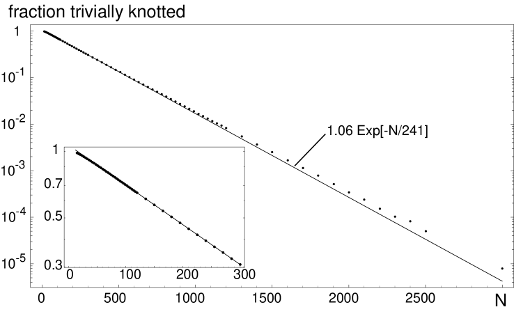
Figure 1: The fraction of loops generated with trivially knotted topology followed the well known exponential form as a function of loop length $N$. Deviation from the fit line at large $N$ is due to the incompleteness of topological invariants employed and reflects the contamination of the supposedly trivial pool with some non-trivial knots. The inset shows the same data for the interval of $N$ up to $300$, where third degree Vassiliev invariant was used along with second degree Vassiliev and Alexander invariants.

We now approach the central issue of this paper, which is our data on the gyration radius of loops, as plotted in Figure 2. To begin with, as a consistency check, at each $N$ we look at the $\langle R_{g}^{2}\rangle_{\rm all}$ averaged over all generated loops, irrespective of their topology. As the upper inset of Figure 2 indicates, the swelling parameter, defined as $\langle R_{g}^{2}\rangle_{\rm all}/(N\ell^{2}/12)$, is practically independent of $N$. Since $N\ell^{2}/12$, as we pointed out before, is the mean square gyration radius for Gaussian loops, this result confirms the statistically representative character of our loop ensemble.

Similar swelling parameter for trivial knots, $\langle R_{g}^{2}\rangle_{\rm triv}/(N\ell^{2}/12)$ is shown in the same upper inset of Figure 2. A few points independently collected by A.Vologodskii VOLOGODSKII_private using only the Alexander invariant are shown as stars, they agree with our data. The data demonstrate clearly that loops with trivial knot topology are on average much more extended than other loops.

To move beyond this qualitative conclusion to the quantitative characterization of topology-driven swelling, we found it necessary to look closer at the errors caused by the contamination of the trivial knots pool due to mistaken assignment of some non-trivial knots as trivial due to insufficiently powerful topological invariants. We used the following procedure to correct for this problem of trivial ensemble contamination.

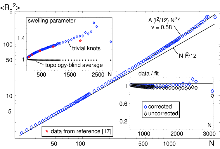
Figure 2: Gyration radius averages over trivially knotted loops, and, as a control, over all loops. The trivial knot average exhibits power law behavior at large $N$ similar to that experienced by polymers which have excluded volume. This topology driven swelling is seen to develop beyond the critical length $N_{0}=241$. Independently collected data of VOLOGODSKII_private is shown by stars ($\star$) and agrees with our results. Upper Inset: Swelling parameter, $\langle R_{g}^{2}\rangle_{\rm all}/(N\ell^{2}/12)$, averaged over all loops irrespective of their topology, shows no dependence on $N$, lending credence to our loop statistics. By contrast, swelling parameter $\langle R_{g}^{2}\rangle_{\rm triv}/(N\ell^{2}/12)$ demonstrates that trivial knots on average swell significantly above the Gaussian average size $N\ell^{2}/12$. Lower Inset: Trivially knotted gyration radius average normalized by power law fit to data. Solid lines demarcate $\pm 5\%$ deviation of data from fit. The small difference between corrected (see formula (8)), and raw trivial knot gyration radius suggests that errors in knot assignment do not significantly affect the scaling power $\nu$.

Let $w=w_{\rm triv}=w_{0}\exp(-N/N_{0})$, the true probability of finding a trivial knot. Then, the averaged gyration radius for all loops (which is equal to $N\ell^{2}/12$) reads

$$\langle R_{g}^{2}\rangle_{\rm all}=\frac{N\ell^{2}}{12}=w\langle R_{g}^{2}\rangle_{\rm triv}+(1-w)\langle R_{g}^{2}\rangle_{\rm non-triv}\ .$$ (6)

Now let $\delta$ be the probability of a non-trivial knot mistakenly assigned as trivial. In Figure 1, $\delta$ is visible as the vertical distance the data points rise above the fit line. The fraction of loops to which we assign, correctly or mistakenly, the trivial status is $w+\delta$. The conditional probabilities of the loop to be a trivial or non-trivial knot provided it is assigned trivial status by our imperfect topological invariants are $w/(w+\delta)$ and $\delta/(w+\delta)$, respectively. Accordingly, the gyration radius averaged over thus contaminated trivial pool, $\langle R_{g}^{2}\rangle^{\prime}_{\rm triv}$ , can be described as the weighted average of loops which either posses or lack trivial knot topology, thus,

$$\langle R_{g}^{2}\rangle^{\prime}_{\rm triv}=\langle R_{g}^{2}\rangle_{\rm triv}\frac{w}{w+\delta}+\langle R_{g}^{2}\rangle_{\rm non-triv}\frac{\delta}{w+\delta}.$$ (7)

Implicit here is an assumption that mistakenly identified knots have the same average gyration radius $\langle R_{g}^{2}\rangle_{\rm non-triv}$ as all other non-trivial knots. Accepting it, we observe that in the equations (6) and (7) we know everything except $\langle R_{g}^{2}\rangle_{\rm triv}$ and $\langle R_{g}^{2}\rangle_{\rm non-triv}$. We solve these coupled equations to find

$$\langle R_{g}^{2}\rangle_{\rm triv} = \langle R_{g}^{2}\rangle_{\rm triv}^{\prime}+\frac{\delta\left[\langle R_{g}^{2}\rangle_{\rm triv}^{\prime}-\langle R_{g}^{2}\rangle_{\rm all}\right]}{w(1-w-\delta)}\simeq$$ (8)

$$\simeq \langle R_{g}^{2}\rangle_{\rm triv}^{\prime}\left(1+\frac{\delta}{w}\right)-\langle R_{g}^{2}\rangle_{\rm all}\left(\frac{\delta}{w}\right)\ ,$$

where the later simplification makes use of the observation that $\delta\ll w$ everywhere, and that $w\ll 1$ when the correction in question is noticeable (say, at $N>1000$ or so). Thus, we obtain that $\langle R_{g}^{2}\rangle_{\rm triv}$ is somewhat larger than directly measured quantity $\langle R_{g}^{2}\rangle_{\rm triv}^{\prime}$ (because $\langle R_{g}^{2}\rangle_{\rm triv}^{\prime}>\langle R_{g}^{2}\rangle_{\rm all}$) by the amount proportional to $\delta/w$.

Thus corrected data for $\langle R_{g}^{2}\rangle_{\rm triv}$ are presented in the main part of Figure 2 as diamonds ($\diamond$). The data fit well to the simple power law $\langle R_{g}^{2}\rangle_{\rm triv}=A\left(\ell^{2}/12\right)N^{2\nu}$ at $N$ larger than about $N=500$, with best fit parameters $A\approx 0.44\pm 0.03$ and $\nu\approx 0.58\pm 0.02$. This result is fully consistent with theoretical prediction AG_pred in several respects. First and foremost is the very fact of power law dependence of $\langle R_{g}^{2}\rangle_{\rm triv}$ on $N$. Second, the value of exponent $\nu$ matches well that of the self-avoiding walks, thus confirming the des Cloizeaux conjecture conj1 . Third, the range of $N$ where the power law is observed supports the idea that it should start at $N>N_{0}$, as in formula (1). Fourth, the value of prefactor $A$ agrees with prediction (3) which is $A\approx 0.42$, thus providing for smooth cross-over at $N$ close to $N_{0}$, as expected.

The fit quality is addressed in the lower inset of the Figure 2, where $\left.{\rm data}\right/{\rm fit}$ is plotted against $N$. Overall, data remain within $\pm 5\%$ of the fit. Importantly, the difference between corrected (see formula (8) ) and uncorrected data is within the $5\%$ error corridor, thus suggesting that the fit result is reliable and is not affected dramatically by the inevitable errors of knot identification.

At the same time, we should point out that within the $5\%$ corridor, our data exhibit small but systematic bend upwards. Formally, this leads to the observation that power law fitting of only part of our data, starting from a larger $N$, say $N>1000$ or $N>1500$ etc, yields increasing $\nu$, up to the physically absurd values of $0.9$ or so at very large $N$. Of course, these unphysical results come from narrowing windows of data where the statistics are increasingly poor. Nevertheless, currently we do not know if the upward bend of the data curve in Figure 2 is entirely due to the measurement errors, or if it hints to something more serious. In particular, this bend prevents us from meaningfully fitting the data with formula (4). Further work is needed to understand whether data improvement, formula modification, or both is required.

Within our current capabilities, we can use our data to address quite a few more interesting issues. One possibility is to look at the mean square gyration radius of non-trivial knots. Such data are presented in Figure 3. Apart from being pulled to much larger values of $N$, our data in this respect is quite similar to that presented earlier by the Swiss group swiss_PNAS . For every non-trivial knot, the mean squared gyration radius remains smaller than the topology blind average over all loops, $N\ell^{2}/12$, and becomes larger at a certain value of $N$ characteristic for each knot. On theoretical grounds, it was hypothesized RG_style_fitting that the leading term in $N\to\infty$ asymptotics $\langle R_{g}^{2}\rangle\simeq A\left(\ell^{2}/12\right)N^{2\nu}$ should be valid for every particular knot type, with both scaling power $\nu$ and ”amplitude” $A$ independent of the knot type. Indeed, this conclusion seems inevitable considering the fact that any given knot at sufficiently large $N$ is dominated by the stretches which effectively look like parts of a trivial knot (see also Quake ; AG_pred ). Looking at the data, Figure 3, with this theoretical concept in mind, we see that the sizes of all knots considered do approach each other with increasing $N$. However, this happens quite slowly even when $N$ is as large as, say, $N=1500\approx 6N_{0}$.

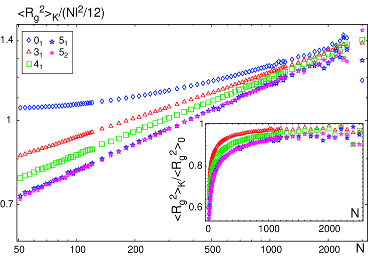
Figure 3: Log-log plot of the mean square gyration radius, $\langle R_{g}^{2}\rangle_{\kappa}$, of knot type $\kappa$, normalized by the topology blind average over all loops for several particular knot types. The inset, which shows the ratio of a particular knot gyration radius to the trivial knot gyration radius, $\langle R_{g}^{2}\rangle_{0}$, demonstrates that all knots remain smaller than, but approach the size of trivial knots.

Our data allow us to make one more step and to look not only at the averaged value of $R_{g}^{2}$ for trivial and some non-trivial knots, but also at the entire probability distributions. We were able to generate and analyze histograms of quality (i.e. looking smooth when plotted) for loops of size $N\leq 600$, where contamination of the trivial pool and the corresponding correction (8) are totally insignificant. Predictably, the probability distributions are different for different topological classes, such as all loops versus loops of a certain knot type ${\cal K}$. Also predictably, the probability distributions of $R_{g}^{2}$ spread out as $N$ increases. The latter observation suggests the idea of looking at the probability distributions of the re-scaled variable $\rho=R_{g}^{2}/\langle R_{g}^{2}\rangle$, where the normalization factor $\langle R_{g}^{2}\rangle$ is taken separately for each $N$ and for each topological entity.

Our main findings are summarized in Figure 4, where we present probability distributions $P(\rho)$ for the trivial knots $0_{1}$ ($\diamond$), trefoils $3_{1}$ ($\Delta$), and $4_{1}$ knots ($\Box$). The data shown are for $N=90$, where high quality statistics were most easily attainable: each histogram is the result of more than $20$ million loops.

In the same figure 4, we plot also for comparison the analytically computed probability distributions for linear chains and for all loops. For linear chains, the necessary distribution $P_{\rm linear}(\rho)$ was found by Fixman a long time ago Fixman . He showed that the corresponding characteristic function (Fourier transform of probability density) is equal to $K_{\rm linear}(s)=\left(\sin z/z\right)^{-3/2}$, where $z^{2}=4\imath s$, and where $s$ is conjugate to $\rho$ (i.e., Fourier transform involves $e^{\imath s\rho}$). We were able to derive similar expression for the probability distribution over all loops, irrespective of topology. In this case, the characteristic function reads $K_{\rm all\ loops}(s)=\left(2\sin(z/2)/z\right)^{-3}$, where $z^{2}=8\imath s$, with the same definition of $s$. Numerical inversion of Fourier transforms yield the curves presented in Figure 4. To avoid overloading the figure, we do not show the corresponding data points obtained for linear chains and for all loops, but they all sit essentially on top of the theoretical curves (which is comforting, as it confirms once again the ergodicity of our loop generation routine).

Comparing the shapes of probability distributions for all loops and those with identified topology, we notice that the latter distributions are somewhat more narrow. Although the effect looks small for the eye, it is certainly there, and it is well above the error bars of our measurements. This means simple knots are less likely to swell much above their average size than other knots, and they are also less likely to shrink far below their average, again compared to other knots.

The latter point is of particular interest given its relation to all problems involving collapsed polymers, such as proteins. Closer look at the small $R_{g}$ region of the probability distribution is presented in the upper inset of Figure 4. There, the probability distributions are plotted in the semi-$log$ scale against $1/\rho$. This can be also understood as the plot of ”confinement” entropy, which corresponds to the squeezing the polymer to within certain (small) radius. The reason why we plot the data against $1/\rho$ is because both $P_{\rm linear}(\rho)$ and $P_{\rm all\ loops}$ at small $\rho$ have asymptotics $\sim\exp\left(-{\rm const}/\rho\right)$, which corresponds to confinement entropy $\sim 1/\rho$, and which can be established by a simple scaling argument, as described, e.g., in AG_Red (page 42). This $1/\rho$ behavior is seen clearly in the upper inset in Figure 4. Furthermore, we see indeed that compressing any specific knot, trivial or otherwise, is significantly more difficult than compressing a phantom loop. Analytical expression of entropy for knots is not known, only the $R_{g}^{-3}\sim\rho^{-3/2}$ scaling at small $\rho$ was conjectured in the work crumpled . Although our data is qualitatively consistent with this prediction in terms of the direction of the trend, more data is needed for quantitative conclusion.

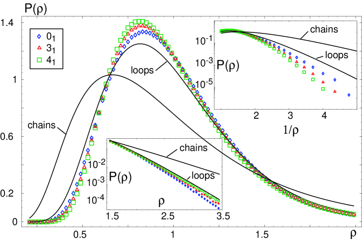
Figure 4: Probability density plots for chains (line, Fixman ), all loops (another line), and loops with certain knots ($0_{1}$ - $\diamond$, $3_{1}$ - $\Delta$, $4_{1}$ - $\Box$). Distributions are presented in terms of the scaling variable $\rho=R_{g}^{2}/\langle R_{g}^{2}\rangle$. Lower Inset: Semi-log probability density plot (or linear entropy plot) at large $\rho$. Upper Inset: Semi-log probability density plot (or linear entropy plot) at small $\rho$ against $1/\rho$.

To conclude, we want to speculate on some broader implications of our findings. To this end, it seems obvious that for any given knot ${\cal K}$, the final asymptotics of $\langle R_{g}^{2}\rangle_{\cal K}$ at $N\to\infty$ are governed by the same exponent $\nu$ as for the trivial knots, that is, according to our results above, $\nu_{\cal K}=\nu_{\rm triv}=\nu_{\rm SAW}\approx 0.589\approx 3/5$. To explain this point, and also to understand at which $N$ this asymptotics takes over, it is useful to compare the polymers with quenched and annealed topology, the latter being simply phantom. At every $N$, the polymer with annealed topology samples a certain ensemble of knots; as $N$ grows longer, the set of knots which are sampled becomes more diverse. In a loose sense, we can imagine a certain average for this set of knots, something like average number of knots, or average knot complexity. For instance, we can average diameter of maximally inflated tube inflated_tube or minimal rope length rope_length . Let us denote ${\cal K}^{\star}(N)$ as the average, or typical knot for the given length $N$. Clearly, as $N$ increases the typical knot gets more complex, its rope length increases, and its inflated diameter decreases. Now let us go back and consider the real polymer of the given length $N$ with real quenched knot topology, ${\cal K}$. We should recognize the important difference between the cases when given knot ${\cal K}$ is more complex (with longer rope length or smaller tube diameter) or simpler (with shorter rope length or larger tube diameter) than ${\cal K}^{\star}(N)$. In the former case, our real polymer can be called overknotted, because it contains larger amount of knots than it would do spontaneously if allowed. In the latter case, the polymer can be called underknotted, because it has fewer knots than typical for its length. Overknotted polymers should be more compact compared to the annealed, or phantom loop; in other words, for them we expect $\langle R_{g}^{2}\rangle_{\cal K}<N\ell^{2}/12$. By contrast, underknotted polymers should be more swollen compared to their phantom counterparts, $\langle R_{g}^{2}\rangle_{\cal K}>N\ell^{2}/12$. In the light of this consideration, we can now understand what happens if we have a given non-trivial knot ${\cal K}$ and we increase $N$. At the beginning, $N$ is small and we are in the overknotted regime. Eventually with growing $N$ we expect to cross over into the underknotted regime, and it is in this regime that we expect the size of the knot to scale as $N^{\nu}$, because every underknotted loop consists basically of very long pieces which are not entangled with each other and are not knotted themselves. The number of such pieces depends on the knot ${\cal K}$, but does not depend on $N$, such that their length scales as $N$ and their size, therefore, must scale as $N^{\nu}$. Much work is needed to make these considerations more quantitative and less speculative, a start in this direction would be to define ${\cal K}^{\star}(N)$ in a more rigorous fashion. Among other things relevant here, the issue of knots localization localization_1 ; localization_2 ; localization_3 must be quantified and incorporated.

To summarize, we have presented simulation data on the sizes of loops with the topologies of trivial or non-trivial knots, for the lengths of up to $3000$ segments. We found that topological constraints have marginal effect on the loop size as long as the loop is shorter than the characteristic length of random knotting, which is about $250$. At larger $N$, our results for trivial knots are consistent with crossing over into the scaling regime $R_{g}\sim N^{\nu}$ analogous to self-avoiding walks statistics, for which $\nu\approx 0.59$. Our findings are also consistent with the idea that the size of any particular non-trivial knot becomes asymptotically equal to that of the trivial knot at very large $N$, although our data suggest the slow decaying approach to this asymptotic regime. Finally, looking at the probability distributions of the (properly re-scaled) loop sizes, we found that topologically complex loops are less likely to adopt either strongly collapsed or strongly expanded configurations.

We wish to thank A. Vologodskii for sharing with us his unpublished data VOLOGODSKII_private . We also acknowledge fruitful discussion with T. Deguchi.

References

- (1) des Cloizeaux, J. (1981) J. Phys. Lett. 42, L433.
- (2) For the polymer with segments of the length and diameter , the excluded volume effect does not lead to appreciable swelling as long as AG_Red . For dsDNA at a reasonable ionic strength, this implies chain length up to about segments, or base pairs.
- (3) Grosberg, A. (2000) Phys. Rev. Lett. 85, 3858-3861.
- (4) Grosberg, A.Y., Khokhlov, A.R. (1994) Statistical Physics of Macromolecules, (AIP Press), pp24-27.
- (5) Koniaris, K., Muthukumar, M. (1991) Phys. Rev. Lett. 66, 2211-2214.
- (6) Deguchi, T., Tsurusaki, K. (1997) Phys. Rev. E. 55, 6245-6248.
- (7) Deutsch, J.M. (1999) Phys. Rev. E. 59, 2539-2541.
- (8) Dobay, A., Dubochet, J., Millett, K., Sottas, P., Stasiak, A. (2003) Proc. Natl. Acad. Sci. USA 100, 5611-5615.
- (9) Matsuda, H., Yao, A., Tsukahara, H., Deguchi, T., Furuta, K., Inami, T. (2003) Phys. Rev. E. 68, 011102.
- (10) Shimamura, M.K., Deguchi, T. (2002) Phys. Rev. E. 65, 051802.
- (11) Orlandini, E., Tesi, M., van Rensburg, E.J., Whittington, S. (1998) J. Phys. A. 31, 5953-5967.
- (12) A similar simpler method applicable for even and re-shuffling vectors obtained from zero sum pairs yields the loops with overlapping nodes. This happens when the re-shuffling results in the succession of some vectors belonging to exactly pairs and thus forming the zero sum (i.e., closed) sub-loop. The probability of such event is of order unity, because the probability for the two vectors from the same pair to be next to each other after the re-shuffling scales as , and there are such pairs; more accurate calculation combinatorics shows that this probability approaches as . For the triangles, there is no such problem, because the probability for the three vectors of the triplet to be next to each other scales as , while the number of triangles is still , so the overlapping loops are rare as (and the probability to have two, or, in general, triplets to occupy completely the stretch of the re-shuffled sequence does not change the estimate).
- (13) Flajolet, P., Noy, M. (2000) in Formal Power Series and Algebraic Combinatorics, eds. Mikhalev, A. V., Krob, D., Mikhalev, A. A. (Springer), pp. 191-201.
- (14) Adams, C. C. (1994) The Knot Book: an Elementary Introduction to the Mathematical Theory of Knots, (W.H. Freeman).
- (15) Lua, R., Borovinskiy, A.L., Grosberg, A.Y. (2004) Polymer 45, 717-731.
- (16) In the work koniaris_muthu_N0 , authors look at the chain with some excluded volume, or thickness ; their results for dependence on approach ours when extrapolated to . The work deguchi_N0 examined Gaussian random polygons, i.e., Gaussian distributed length of segments.
- (17) A. Vologodskii, private communication.
- (18) Quake, S. (1994) Phys. Rev. Lett. 73, 3317.
- (19) Fixman, M. (1962) J. Chem. Phys. 36, 306-310.
- (20) Grosberg, A.Y., Nechaev, S.K., Shakhnovich, E.I. (1988) Le Journal de Physique (France) 49, 2095-2100.
- (21) Grosberg, A.Y., Feigel, A., Rabin, Y., (1996) Phys. Rev. E. 54, 6618-6622.
- (22) Stasiak, A., Katritch, V., Kauffman, L.H. (1999) Ideal Knots, (World Scientific Publishing Company).
- (23) Katrich, V., Olson, W.K., Vologodskii, A., Dubochet, J., Stasiak A. (2000) Phys. Rev. E. 61, 5545.
- (24) Metzler, R., Hanke, A., Dommesrnes, P.G., Kantor, Y., Kardar, M. (2002) Phys. Rev. Lett. 88, 188101.
- (25) Hanke, A., Metzler, R., Dommesrnes, P.G., Kantor, Y., Kardar, M. (2003) European Phys. Journal E 12, 347-354.