Approximating the satisfiability transition by suppressing fluctuations.

Abstract

Using methods and ideas from statistical mechanics and random graph theory, we propose a simple method for obtaining rigorous upper bounds for the satisfiability transition in random boolean expressions composed of $N$ variables and $M$ clauses with $K$ variables per clause. The method is based on the identification of the core – a subexpression (subgraph) that has the same satisfiability properties as the original expression. We formulate self-consistency equations that determine the macroscopic parameters of the core and compute an improved annealing bound for the satisfiability threshold, $\alpha_{c}=M/N$. We illustrate the method for three sample problems: $K$-XOR-SAT, $K$-SAT and positive $1$-in-$K$-SAT.

I Introduction

Over the past decade the statistical properties of combinatorial problems has attracted increasingly greater attention from both the computer science and physics communities ksat1 ; ksat2 ; ksat3 . Most computationally difficult problems encountered in practice belong to the class of NP-complete problems. There is a one-to-one correspondence between these problems and spin glass models fu . Unlike problems with regular structure, many combinatorial optimization problems are formulated on random graphs and hypergraphs. The long-standing problem in the computer science community is “P vs. NP”, that is, can NP-complete problems be solved in polynomial time, or they are inherently intractable karp ? Although the problem is extremely important, it is also deeply theoretical as it concentrates on worst-case scenarios. From the viewpoint of practitioners, efficient algorithms have to be designed with real-world problems in mind. Appropriate test cases can be prepared for comparing the performance of different algorithms. However, this approach does not allow the design of algorithms with typical performance in mind, only their comparison.

One can argue that the purely theoretical study of algorithms was somewhat impeded by exploding speed of computers that encouraged experimentation. This state of affairs may be challenged by the emerging paradigm of quantum computing. Until a working prototype of a quantum computer is built, it exists only on paper. Classical simulations of quantum computers can be done only for very small problems, due to speed and memory requirements. Since these reqirements grow exponentially with the size of the problem, they could be used only in proof-of-concept scenarios. While quantum computation was shown to be efficient for some classically intractable problems (the most notable example being Shor’s algorithm shor ), whether they provide an advantage for NP-complete problems is unresolved. Therefore, designing algorithms with typical complexity in mind for quantum computer may be desirable. Whether the newly proposed quantum adiabatic algorithm is efficient in tackling NP-complete problems is an area of active research farhi ; vazirani ; hogg .

The statistics of real-world examples is largely unknown. As a first approximation one can assume that the problems can be chosen completely at random. The underlying belief is that if an algorithm is efficient for a uniform ensemble of randomly chosen problem instances, it will solve real-world examples fairly efficiently as well. The performance for random problems is a truly unbiased benchmark to compare different algorithms. The same explosion in computational speed responsible for diminished reliance on theoretical study has also reignited interest in this type of study.

Many problems of interest are written as a boolean expression (a formula) – a set of $N$ variables and $M$ constraints, all which we aim to satisfy. Each constraint is a clause involving $K$ variables and it determines which combinations of variables are permitted. The types of constraints differ from problem to problem, but for great many the following picture persists: for small $\alpha=M/N$ the problem is almost always (that is, with probability $1$ in the limit $N\rightarrow\infty$) satisfiable, while at $\alpha=\alpha_{c}$ an abrupt change occurs, and for all $\alpha>\alpha_{c}$ the problem is almost always unsatisfiable ksat1 ; ksat2 ; ksat3 . An even more interesting phenomenon occurs for the typical running time of the algorithm: the time it takes to solve a problem is usually polynomial for $\alpha<\alpha_{d}<\alpha_{c}$, and exponential for $\alpha>\alpha_{d}$, where $\alpha_{d}$ is algorithm-dependent. However, independent of the algorithm used, the complexity peaks at $\alpha=\alpha_{c}$, where the probability that the formula is satisfiable is approximately $1/2$.

Random satisfiability problems grabbed the attention of the statistical physics community, since the phenomenon in question is a phase transition; the study of this phase transition may improve the understanding of the physics of random materials such as glasses. This is in addition to any statistical properties of the solutions – properties that can be used for the design of efficient classical or quantum algorithms.

The quest for exact values of $\alpha_{c}$ or $\alpha_{d}$ has so far been elusive. The best results for a particular problem – K-SAT – were obtained using the so-called one-step RSB approximation and are in excellent agreement with experiment ksat1rsb . However, the method has drawn criticism because the method itself is not well-understood, lacks a rigorous foundation, and the result depends on extensive numerical computations. On the upside, rigorous bounds have been obtained for $K$-XOR-SAT (note, however that it can be solved in polynomial time). On the mathematical side, a series of results on rigorous lower lower and upper upper bounds on $\alpha_{c}$ appeared recently. Typically lower bounds rely on an explicit algorithm and upper bounds rely on the counting of solutions. The trivial upper bound is obtained using the annealing approximation. All improvements over the annealing approximation employ the fact that at the satisfiability transition the number of solutions jumps from the exponentially large number $2^{\alpha N}$ to $0$. The method we propose in this paper does not deviate from this strategy. For any random formula we identify a subformula that possesses identical satisfiability properties, but has suppressed fluctuations. That is, if the formula is satisfiable, the subformula is also satisfiable but has a significantly smaller number of solutions. By performing the disorder average of the number of solutions of the subformula (rather than formula, as in the annealing approximation) the point where the average goes to zero determines the upper bound on the true transition point.

The advantages of the method described here are that it is rigorous (it does not rely on any hypotheses, although we supply proofs only when they are not immediately intuitive; it is straightforward to rederive all the results with complete mathematical rigor) and that the method is applicable to various types of random satisfiability problems. We choose to describe $K$-XOR-SAT as well as the NP-complete problems $K$-SAT and positive $1$-in-$K$-SAT. Each problem adds its own “touch” to the formalism. For the case $K$-XOR-SAT – a polynomial problem – the upper bound is exact kxorsat , while the upper bound for $K$-SAT grossly overestimates the transition. This could be related to the fact that $K$-SAT is very difficult for classical algorithms. In all cases we take a two step approach. In the first step we compute the parameters of the subformula – the core. In the second step we compute the annealing approximation for the number of solutions of the subformula. The size of the core also exhibits a phase transition and has been studied for a range of problems pittel . Our method provides a much simpler way to derive those results.

The paper is organized as follows. We describe $K$-XOR-SAT, $K$-SAT and positive $1$-in-$K$-SAT in sections II through IV; section V is devoted to numerical simulations for the positive $1$-in-$3$-SAT problem; section VI is a summary.

II $K$-XOR-SAT

In this model the instance of the problem consists of $N$ variables and $M$ clauses, each clause involving $K$ variables. Each variable can take values $0$ or $1$. The ensemble we consider (random hypergraph) is that of independent clauses with variables in each clause drawn uniformly at random out of the set of $N$ variables. To each clause we also attribute a number $0$ or $1$, each with probability of $1/2$, and posit that the clause is satisfied if the exclusive-or (XOR) of the $K$ variables in the clause equals that number. The entire formula is said to be satisfied if all of its clauses are satisfied

The probability that such random formula is satisfied, in the limit $N\rightarrow\infty$, exhibits a sharp jump from $1$ to $0$ at some critical ratio of clauses to variables $\alpha_{c}=M/N$. We attempt to estimate this satisfiability threshold. The simplest approximation (in fact an upper bound) uses the first moment method (known as the annealing approximation in the physics community). One can compute the disorder-averaged number of solutions. The point where the expectation value of the number of solutions becomes smaller than $1$ corresponds to a formula that is unsatisfiable; therefore this serves as an upper bound on the location of the transition. In essence we have approximated $\mathbbm{P}(\textrm{sat})\equiv\mathbbm{P}[\mathcal{N}\geqslant 1]=\mathbbm{E}[\theta(\mathcal{N}-1)]$ by $\mathbbm{E}[\mathcal{N}]$, where $\mathcal{N}$ denotes the number of solutions (an integer). In the physics community the annealing approximation for the entropy is regarded as the replacement of the correct quantity $\mathbbm{E}[\ln\mathcal{N}]$ by the incorrect expression $\ln\mathbbm{E}[\mathcal{N}]$.

Computing the point where the annealed entropy becomes zero is trivial. For each clause, the probability that the clause is satisfiable is independent of the assignment of variables and equals $1/2$. Therefore the expected number of solutions is

$$\mathbbm{E}[\mathcal{N}]=2^{N}2^{-M},$$ (1)

and the corresponding entropy $S_{\textrm{ann}}=N\ln 2-M\ln 2$ becomes negative above $\alpha_{u}=1$ (the subscript indicates that this is the upper bound).

II.1 Concept of a core

A major drawback of the annealing approximation is in that it fails to account for finite entropy at the satisfiability transition. (By accident, for this particular problem, the annealed expression for the entropy on the satisfiable side of the transition is exact). It can be argued that at any finite connectivity a random graph possesses a large ($O(N)$) number of variables that do not appear in any clauses, thus making a contribution to the entropy which we fail to take into account. Furthermore, there are clauses that involve variables, the variables not being in any other clauses, as well as small clusters of such clauses. The annealing bound would be significantly improved if it were possible to separate these irrelevant contributions to the entropy.

In a paper devoted to the finite-size effects of the satisfiability transition, a concept of irrelevant clauses was put forward. Given a random formula one can always easily identify clauses that can be trivially satisfied. The paper did not specify the procedure for finding such clauses, only that their number is extensive ($O(N)$). One example is isolated clauses, since variables can always be set so as to satisfy the clause. The presence of such extensive clauses is responsible for the lower bound of $2$ of the finite-size scaling exponent $\nu$, or, in other words, that the disorder is relevant to the phase transition.

One can try to advance the most general definition of irrelevant clause based on local properties alone. In fact this has been done for $K$-XOR-SAT kxorsat . In essence we repeat the derivation in a slightly simplified form, but will generalize it to other problems later on. For $K$-XOR-SAT we identify variables that appear in no clauses and delete those variables. Further, we identify variables that appear in only one clause. Such variables can be set to $0$ or $1$ (after other variables have been assigned) so that the clause becomes satisfiable. Hence the satisfiability of the entire formula will be unaffected if the variable and the corresponding clause are deleted. This process (known as trimming algorithm, illustrated below, in Fig. 1) can be continued until we either end up with an empty graph (which would imply that the formula is satisfiable) or a core – the formula in which all variables appear in at least two clauses. One can compute the annealed entropy on the core and use the point at which the entropy becomes zero as the improved upper bound $\alpha_{u}^{\prime}$.

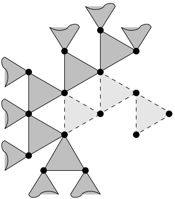
Figure 1: Example of trimming algorithm for 3-XOR-SAT. Variables are represented graphically as vertices and clauses are represented as triangles. Incomplete triangles represent connections to the remainder of the graph (not shown). Lightly shaded clauses are removed by the trimming algorithm.

We examine the structure of the remaining core. First, observe that the remaining core does not depend on the order in which the variables and clauses are removed. In fact the remaining core is the unique maximal subformula of the original formula with the property that every variable appears in at least two clauses. The original formula is the core plus all deleted clauses and variables. Assume that the core has $N^{\prime}$ variables and $M^{\prime}$ edges (implying $N-N^{\prime}$ variables and $M-M^{\prime}$ clauses were deleted). Correspondingly, all original graphs can be divided into distinct groups based on values of $N^{\prime}$, $M^{\prime}$. Suppose we keep $N^{\prime}$ and $M^{\prime}$ fixed. Observe that to every realization of the core there corresponds an equal number of possible realizations of deleted clauses, and, as a consequence, an equal number of possible realizations of the original graph (in the group labeled by $N^{\prime}$, $M^{\prime}$). Therefore, for any fixed $N^{\prime}$, $M^{\prime}$ all possible realization of the core are equiprobable – a fact we employ to perform disorder averages.

Notice that all possible realizations of the core are equiprobable only for fixed $N^{\prime}$, $M^{\prime}$. The values of $N^{\prime}$ and $M^{\prime}$ themselves fluctuate. However, the fluctuations in $N^{\prime}$ and $M^{\prime}$ are on the order of $O(\sqrt{N})$ while their respective values are $O(N)$. Since we expect the threshold to be sharp as a function of $M^{\prime}/N^{\prime}$, we need not concern ourselves with these fluctuations. Therefore we concentrate on finding the most likely values of $N^{\prime}/N$ and $M^{\prime}/N$. One approach is to work with a set of $\{c_{k}\}$ – a fraction of vertices that appear in $k$ clauses. One can describe an algorithm as a random process and study the changes in the average values of $\{c_{k}\}$. The discrete steps of the algorithm are approximated by continuous time $t$, and a set of $\{c_{k}(t)\}$ is replaced by its generating function $c(t,x)=\sum_{k}c_{k}(t)x^{k}$. The problem is then reduced to solving the resulting PDE. This is the approach taken in kxorsat . Slightly differing variants of this method were also employed in pittel ; trim1 ; trim2 . We instead opt for an approach that does not take dynamics into considerations. The approach is inspired in part by work analyzing the matching problem karpsipser .

In essence, we seek the disordered average of $N^{\prime}/N$. This is precisely the probability $p$ that a randomly chosen variable belongs to the core. We can also fix a specific variable (say, variable $x_{0}$) and perform a disorder average of a function that yields $1$ if that vertex belongs to the core or $0$ if it does not. For every formula $\mathcal{F}$ we can introduce the set $\mathcal{C}$ of variables that belong to the core. Obviously $|\mathcal{C}|\equiv N^{\prime}=pN$. Now, introduce an extension of $\mathcal{C}$, which we denote as $\mathcal{C}^{\prime}$, defined as the minimal set that satisfies the following requirements

1. $\mathcal{C}\subseteq\mathcal{C}^{\prime}$.

2. If $K-1$ variables in some clause belong to $\mathcal{C}^{\prime}$, then the remaining variable must also belong to $\mathcal{C}^{\prime}$.

It is straightforward to see that set $\mathcal{C}^{\prime}$ so defined is unique. Let $|\mathcal{C}^{\prime}|=qN$, where $q$ can be interpreted as the probability that a random vertex belongs to $\mathcal{C}^{\prime}$.

Let us turn to the original random graph. The number of clauses in which the variable $x_{0}$ appears is a random variable distributed according to a Poisson distribution with parameter $K\alpha$. In performing disorder averages we can first average over all possible disorders with fixed values of clauses $k$ first, and average over $k$ with weight $\mathrm{e}^{-K\alpha}(K\alpha)^{k}/k!$ as the last step. Further, observe that those $k$ clauses are independent. Let $\mathcal{F}^{\prime}$ denote a formula that is obtained by removing the variable $x_{0}$ and the clauses in which it appears. Let $q^{\prime}$ denote the parameter $q$ associated with $\mathcal{F}^{\prime}$. Suppose that for some clause in which $x_{0}$ appears, all the other $K-1$ variables belong to $\mathcal{C}^{\prime}[\mathcal{F}^{\prime}]$. Then $x_{0}$ must belong to $\mathcal{C}[\mathcal{F}]$. The probability that for some clause $K-1$ variables other than $x_{0}$ belong to $C^{\prime}[\mathcal{F}^{\prime}]$ is $(q^{\prime})^{K-1}$. The number of such clauses is, hence, also Poisson, but with parameter $K\alpha(q^{\prime})^{K-1}$. The probability $q$ that $x_{0}$ belongs to $\mathcal{C}[\mathcal{F}]$ is therefore

$$q=\sum_{k=1}^{\infty}\mathrm{e}^{-K\alpha(q^{\prime})^{K-1}}\frac{\left(K\alpha(q^{\prime})^{K-1}\right)^{k}}{k!}=1-\mathrm{e}^{-K\alpha(q^{\prime})^{K-1}}.$$ (2)

Now observe that $\mathcal{F}^{\prime}$ is essentially a random formula with $N-1$ variables and the same (to within $O(1/N)$) ratio of clauses to variables. Therefore in the limit $N\rightarrow\infty$ which we are ultimately interested in, there should be no difference in statistical properties, and hence $q=q^{\prime}$. This leads to self-consistency equation

$$q=1-\mathrm{e}^{-K\alpha q^{K-1}}.$$ (3)

Note that $q=0$ is always a solution to this equation. Since the core is defined as the largest possible subformula with certain properties, and the size of the core is directly related to $q$, we must adopt a convention that the largest possible solution to (3) is always chosen. Below a certain threshold only $q=0$ is a solution, whereas above the threshold, another $q>0$ solution appears.

We now turn to the original goal of finding $N^{\prime}$. If at least two clauses which include $x_{0}$ have the property that $K-1$ other variables are in $\mathcal{C}^{\prime}[\mathcal{F}^{\prime}]$, then the variable $x_{0}$ as well as the aforementioned variables are in $\mathcal{C}[\mathcal{F}]$. Hence, we can write

$$p=\sum_{k=2}^{\infty}\mathrm{e}^{-K\alpha q^{K-1}}\frac{\left(K\alpha q^{K-1}\right)^{k}}{k!}=1-\left(1+K\alpha q^{K-1}\right)\mathrm{e}^{-K\alpha q^{K-1}}.$$ (4)

To compute $M^{\prime}$ we examine the average degree (number of clauses in which it appears) of the randomly chosen vertex in the core. The latter should equal $KM^{\prime}/N^{\prime}$. If vertex $x_{0}$ is in the core (with probability $p$), the number of clauses which are in the core was shown above to be a random variable – a truncated (only $k\geqslant 2$ are allowed) Poisson distribution with parameter $K\alpha q^{K-1}$. Therefore

$$KM^{\prime}/N^{\prime}=\sum_{k=2}^{\infty}k\mathrm{e}^{-K\alpha q^{K-1}}\frac{\left(K\alpha q^{K-1}\right)^{k}}{k!}\Big{/}\sum_{k=2}^{\infty}\mathrm{e}^{-K\alpha q^{K-1}}\frac{\left(K\alpha q^{K-1}\right)^{k}}{k!}.$$ (5)

Recognizing that the denominator is $p=N^{\prime}/N$ we can rewrite

$$M^{\prime}/N=\frac{1}{K}\sum_{k=2}^{\infty}k\mathrm{e}^{-K\alpha q^{K-1}}\frac{\left(K\alpha q^{K-1}\right)^{k}}{k!}=\alpha q^{K-1}\left(1-\mathrm{e}^{-K\alpha q^{K-1}}\right)=\alpha q^{K}.$$ (6)

II.2 Improved annealing bound

As with the original annealing bound, we are aided by the fact that clauses require that the exclusive-or of the variables be either $0$ or $1$ with probability $1/2$. The probability that a clause is satisfied is independent of the assignment of the variables, and the entropy is predicted to decrease to zero when $M^{\prime}/N^{\prime}=1$ or

$$\alpha q^{K}=q-K\alpha q^{K-1}+K\alpha q^{K}$$ (7)

Coupled with $1-q=\mathrm{e}^{-K\alpha q^{K-1}}$ this puts the upper bound of critical threshold at $\alpha_{u}^{\prime}\approx 0.918$.

It is a remarkable feature of $K$-XOR-SAT is that whenever it is satisfiable, the number of solutions of $K$-XOR-SAT equals the number of solutions of the corresponding “ferromagnetic” model, where we require that the exclusive-or of the variables be precisely $0$ in all clauses. Note that for $K$-XOR-SAT, this is not so; the ferromagnetic model always possesses at least one solution. The next observation is that the disorder average of the square of the number of solutions of $K$-XOR-SAT $\mathbbm{E}[\mathcal{N}^{2}]$ equals $2^{N^{\prime}-M^{\prime}}$ multiplied by $\mathbbm{E}[\mathcal{N}]$ as computed for the ferromagnetic model. As long as the annealing bound for the ferromagnetic model equals that for $K$-XOR-SAT we can be sure that the annealing bound is correct and we are in the satisfiable phase. The point at which it ceases to be so is the lower bound on the satisfiability transition $\alpha_{l}$.

Finding the annealed entropy for the ferromagnetic model on a complete graph is trivial and amounts to finding a maximum of

$$-N\Big{[}\frac{1+m}{2}\ln\frac{1+m}{2}+\frac{1-m}{2}\ln\frac{1-m}{2}\Big{]}+M\ln\frac{1+m^{3}}{2}.$$ (8)

For as long as $m=0$ is a global maximum of this expression, the annealed entropies of the ferromagnetic and random models are equal. It ceases to be so at $\alpha_{l}\approx 0.889$, which serves as a lower bound on satisfiability transition. It is worthwhile to compute the annealed entropy on the core. That task has been accomplished in kxorsat . We rederive the results using a different method which can be readily generalized to other problems.

The annealed entropy is simply the difference between $\ln\mathcal{N}_{s,J}$ and $\ln\mathcal{N}_{J}$, where $\mathcal{N}_{J}$ is the number of possible disorders, and $\mathcal{N}_{s,J}$ counts the total number of disorder configurations and variable assignments compatible with the disorder. For simplicity, we decide to distinguish between disorders that differ only by permutation of clauses and permutation of variables within clauses. Any double counting in $\mathcal{N}_{J}$ due to this convention will be exactly canceled by identical factor in $\mathcal{N}_{s,J}$. The advantages are especially evident for the case of the original random graph. We can immediately obtain $\mathcal{N}_{J}=N^{3M}$. The expression is more complex when restricted so that the degrees of all variables are at least $2$. We now investigate it closely. We introduce a set $\{c_{\boldsymbol{k}}\}$ where $\boldsymbol{k}$ is a vector with $K$ components $\{k_{p}\}$ that count the number of clauses in which some variable appears in $p$-th position. The quantity $c_{\boldsymbol{k}}$ is the fraction of variables described by vector $\boldsymbol{k}$. One trivial constraint is that $\sum_{\boldsymbol{k}}c_{\boldsymbol{k}}=1$. One can represent disorders as an $M^{\prime}\times K$ table of numbers from $1$ to $N^{\prime}$. We can divide the variables into various classes according to the value of $\boldsymbol{k}$. The number of all possible permutations is the product of two factors.

1. $N^{\prime}!\big{/}\prod_{\boldsymbol{k}}N_{\boldsymbol{k}}^{\prime}!$ for the number of ways to arrange the variables into the various classes.

2. $\prod_{p}\left[M^{\prime}!\Big{/}\prod_{\boldsymbol{k}}(k_{p}!)^{N_{\boldsymbol{k}}^{\prime}}\right]$ for the number of ways to rearrange the variables in the $M^{\prime}\times K$ table.

In general we ought to perform a sum over all possible values of $N_{\boldsymbol{k}}^{\prime}$. However, the sum is dominated by particular values of $N_{\boldsymbol{k}}^{\prime}$ that maximize the entropy ($N_{\boldsymbol{k}}^{\prime}=N^{\prime}c_{\boldsymbol{k}}$)

$$S_{J}[c_{\boldsymbol{k}}] = -N^{\prime}\sum_{\boldsymbol{k}}c_{\boldsymbol{k}}\ln c_{\boldsymbol{k}}+K(M^{\prime}\ln M^{\prime}-M^{\prime})-N^{\prime}\sum_{\boldsymbol{k}}c_{\boldsymbol{k}}\Big{(}\sum_{p}\ln k_{p}!\Big{)}$$ (9)

$$= S_{J}^{(1)}[c_{\boldsymbol{k}}]+K(M^{\prime}\ln M^{\prime}-M^{\prime}).$$

Note that we have $K$ constraints on $c_{\boldsymbol{k}}$

$$\sum_{\boldsymbol{k}}k_{p}c_{\boldsymbol{k}}=M^{\prime}/N^{\prime},$$ (10)

and that we require $c_{\boldsymbol{k}}=0$ if $\sum_{p}k_{p}<2$.

Maximizing $S_{J}^{(1)}[c_{\boldsymbol{k}}]$ is easiest if we work with its dual transform. Let $\{-\ln\mu_{p}\}$ be dual variables associated with constraints (10). Instead of finding

$$S_{J}^{(1)}[N^{\prime},M^{\prime}]=\max_{c_{\boldsymbol{k}}}\bigg{\{}S_{J}^{(0)}[c_{\boldsymbol{k}}]\,\bigg{|}\,\sum_{\boldsymbol{k}}k_{p}c_{\boldsymbol{k}}=M^{\prime}/N^{\prime}\bigg{\}}$$ (11)

we compute

$$\tilde{S}_{J}^{(1)}[\{\mu_{p}\}]=\min_{M^{\prime}_{p}}\bigg{\{}-\sum_{p}M_{p}^{\prime}\ln\mu_{p}-S_{J}^{(1)}[N^{\prime},\{M_{p}^{\prime}\}]\bigg{\}},$$ (12)

where $S_{J}^{(1)}[N^{\prime},\{M_{p}^{\prime}\}]$ denotes $S_{J}^{(1)}[c_{\boldsymbol{k}}]$ maximized under the constraints $\sum_{\boldsymbol{k}}k_{p}c_{\boldsymbol{k}}=M_{p}^{\prime}/N^{\prime}$. After simplifications

$$\tilde{S}_{J}^{(1)}[\{\mu_{p}\}]=\min_{\{c_{\boldsymbol{k}}\}}\bigg{\{}-N^{\prime}\sum_{\boldsymbol{k}}c_{\boldsymbol{k}}\sum_{p}k_{p}\ln\mu_{p}+N^{\prime}\sum_{\boldsymbol{k}}c_{\boldsymbol{k}}\ln\Big{[}c_{\boldsymbol{k}}\prod_{p}k_{p}!\Big{]}\bigg{\}}$$ (13)

Optimizing this with respect to $c_{\boldsymbol{k}}$ under the constraint $\sum_{\boldsymbol{k}}c_{\boldsymbol{k}}=1$ and $c_{\boldsymbol{k}}=0$ for $|\boldsymbol{k}|<2$ yields

$$\widetilde{S}_{J}^{(1)}[\{\mu_{p}\}]=-N^{\prime}\ln G\Big{(}\sum_{p}\mu_{p}\Big{)},$$ (14)

where $G(x)=\sum_{k\geqslant 2}x^{k}/k!=e^{x}-1-x$ is the generating function of the ensemble. Reverting to original variables is easy. Via the dual transform we obtain

$$S_{J}^{(1)}[N^{\prime},M^{\prime}]=\min_{\{\mu_{p}\}}\bigg{\{}-M^{\prime}\sum_{p}\ln\mu_{p}+\tilde{S}_{J}^{(1)}[\{\mu_{p}\}]\bigg{\}},$$ (15)

and for $\ln N_{J}$ we obtain

$$S_{J}[N^{\prime},M^{\prime}]=\min_{\{\mu_{p}\}}\bigg{\{}M^{\prime}\sum_{p}\ln\frac{M^{\prime}}{\mu_{p}}+N^{\prime}\ln G\Big{(}\sum_{p}\mu_{p}\Big{)}\bigg{\}}-KM^{\prime}.$$ (16)

Clearly, the minimum is permutation-symmetric: $\mu_{p}=\mu/K$. Equivalently,

$$S_{J}[N^{\prime},M^{\prime}]=\min_{\mu}\left\{KM^{\prime}\ln\frac{KM^{\prime}}{\mu}+N^{\prime}\ln G(\mu)\right\}-KM^{\prime}.$$ (17)

Comparison with (3), (6) gives $\mu=K\alpha q^{K-1}$. Note that substituting $G(x)=e^{x}$ (meaning no constraints on degrees of variables) gives $\mu=KM^{\prime}/N^{\prime}$ and $S_{J}[N^{\prime},M^{\prime}]=KM^{\prime}\ln N^{\prime}$ as expected.

We now turn to computing the logarithm of $\mathcal{N}_{s,J}$. Binary variables can take values of $0$ and $1$. Since these can be mapped onto $+1$ and $-1$, with exclusive-or replaced by a product, from now on we shall succinctly refer to values taken by variables as $+$ and $-$. For each realization of disorder and variable assignment, we ascribe a type $\boldsymbol{\sigma}$ to each clause according to the values of the variables inside that clause; $\boldsymbol{\sigma}$ is a vector with $K$ elements with $\sigma_{p}\in\{+,-\}$. For the time being we fix the number of clauses of each type $M_{\boldsymbol{\sigma}}^{\prime}$ (remember that $M_{\boldsymbol{\sigma}}=0$ unless $\prod_{p}\sigma_{p}=+$ for the ferromagnetic model). In addition to its value $s\in\{+,-\}$, we ascribe to each variable a vector $\boldsymbol{k}$ of $K2^{K}$ elements; $k_{\boldsymbol{\sigma}}^{p}$ denotes the number of clauses of type $\boldsymbol{\sigma}$ in which that variable appears in $p$-th position. Having fixed $M_{\boldsymbol{\sigma}}^{\prime}$ and $N_{s,\boldsymbol{k}}^{\prime}$ we discover that the contribution to $\mathcal{N}_{s,J}$ is given by the product of $3$ factors:

1. $N^{\prime}!\big{/}\sum_{s,\boldsymbol{k}}N_{s,\boldsymbol{k}}^{\prime}!$ for the number of ways to arrange the variables into classes.

2. $\prod_{p,\boldsymbol{\sigma}}\left[M_{\boldsymbol{\sigma}}^{\prime}!\Big{/}\prod_{s,\boldsymbol{k}}(k_{\boldsymbol{\sigma}}^{p}!)^{N_{s,\boldsymbol{k}}^{\prime}}\right]$ for the number of ways to rearrange the variables within the clauses.

3. $M^{\prime}!\big{/}\prod_{\boldsymbol{\sigma}}M_{\boldsymbol{\sigma}}^{\prime}!$ for the number of ways to assign types to clauses.

The associated entropy

$$S_{s,J}[c_{s,\boldsymbol{k}}]=-N^{\prime}\sum_{s,\boldsymbol{k}}c_{s,\boldsymbol{k}}\ln\Big{[}c_{s,\boldsymbol{k}}\prod_{p,\boldsymbol{\sigma}}k_{\boldsymbol{\sigma}}^{p}!\Big{]}+K\sum_{\boldsymbol{\sigma}}\left(M_{\boldsymbol{\sigma}}^{\prime}\ln M_{\boldsymbol{\sigma}}^{\prime}-M_{\boldsymbol{\sigma}}^{\prime}\right)+M^{\prime}\ln M^{\prime}-\sum_{\boldsymbol{\sigma}}M_{\boldsymbol{\sigma}}^{\prime}\ln M_{\boldsymbol{\sigma}}^{\prime}$$ (18)

is to be maximized under the constraints

$$\sum_{s,\boldsymbol{k}}k_{\boldsymbol{\sigma}}^{p}c_{s,\boldsymbol{k}}=M_{\boldsymbol{\sigma}}^{\prime}$$ (19)

and the requirement that $c_{s,\boldsymbol{k}}=0$ unless $\sum_{p,\boldsymbol{\sigma}}k_{\boldsymbol{\sigma}}^{p}\geqslant 2$. Another important constraint is that unless $\sigma_{p}=s$, we require $k_{\boldsymbol{\sigma}}^{p}=0$.

The optimization of the first part of the entropy is best accomplished through the use of the dual transformation. The dual parameters are $\{-\ln\mu_{\boldsymbol{\sigma}}^{p}\}$:

$$\tilde{S}_{s,J}^{(1)}[\{\mu_{\boldsymbol{\sigma}}^{p}\}] = \min_{\{M_{\boldsymbol{\sigma}}^{p}\}}\bigg{\{}-\sum_{p,\boldsymbol{\sigma}}M_{\boldsymbol{\sigma}}^{p}\ln\mu_{\boldsymbol{\sigma}}^{p}$$ (20)

$$-\max_{\{c_{s,\boldsymbol{k}}\}}\Big{\{}-N^{\prime}\sum_{s,\boldsymbol{k}}c_{s,\boldsymbol{k}}\ln\Big{[}c_{s,\boldsymbol{k}}\prod_{p,\boldsymbol{\sigma}}k_{\boldsymbol{\sigma}}^{p}!\Big{]}\Big{|}\sum_{\boldsymbol{k}}k_{\boldsymbol{\sigma}}^{p}c_{s,\boldsymbol{k}}=M_{\boldsymbol{\sigma}}^{p}\Big{\}}\bigg{\}}.$$

After simplifications we can rewrite

$$\tilde{S}_{s,J}^{(1)}[\{\mu_{\boldsymbol{\sigma}}^{p}\}]=N^{\prime}\ln\bigg{[}G\Big{(}\sum_{p,\boldsymbol{\sigma}}\frac{1+\sigma_{p}}{2}\mu_{\boldsymbol{\sigma}}^{p}\Big{)}+G\Big{(}\sum_{p,\boldsymbol{\sigma}}\frac{1-\sigma_{p}}{2}\mu_{\boldsymbol{\sigma}}^{p}\Big{)}\bigg{]}.$$ (21)

The argument of the first $G$ is a sum restricted to $\sigma_{p}=+$, and the argument of the second $G$ is a sum restricted $\sigma_{p}=-$. It is convenient to introduce

$$\mu_{\pm}=\sum_{p,\boldsymbol{\sigma}}\frac{1\pm\sigma_{p}}{2}\mu_{\boldsymbol{\sigma}}^{p}.$$ (22)

Reverting the dual transformation we can obtain

$$S_{s,J}[N^{\prime},\{M_{\boldsymbol{\sigma}}^{\prime}\}] = \min_{\{\mu_{\boldsymbol{\sigma}}^{p}\}}\bigg{\{}\sum_{p,\boldsymbol{\sigma}}M_{\boldsymbol{\sigma}}^{\prime}\ln\frac{M_{\boldsymbol{\sigma}}^{\prime}}{\mu_{\boldsymbol{\sigma}}^{p}}+N^{\prime}\ln\bigg{[}G\Big{(}\sum_{p,\boldsymbol{\sigma}}\frac{1+\sigma_{p}}{2}\mu_{\boldsymbol{\sigma}}^{p}\Big{)}+G\Big{(}\sum_{p,\boldsymbol{\sigma}}\frac{1-\sigma_{p}}{2}\mu_{\boldsymbol{\sigma}}^{p}\Big{)}\bigg{]}\bigg{\}}$$ (23)

$$-KM^{\prime}+M^{\prime}\ln M^{\prime}-\sum_{\boldsymbol{\sigma}}M_{\boldsymbol{\sigma}}^{\prime}\ln M_{\boldsymbol{\sigma}}^{\prime}.$$

It is convenient to define

$$\mathcal{M}_{\pm}=\sum_{p,\boldsymbol{\sigma}}\frac{1+\sigma_{p}}{2}M_{\boldsymbol{\sigma}}^{\prime}.$$ (24)

The expression for the entropy can be simplified to

$$S_{s,J}[N^{\prime},\{M_{\boldsymbol{\sigma}}^{\prime}\}] = \min_{\mu_{\pm}}\left\{\mathcal{M}_{+}\ln\frac{\mathcal{M}_{+}}{\mu_{+}}+\mathcal{M}_{-}\ln\frac{\mathcal{M}_{-}}{\mu_{-}}+\ln[G(\mu_{+})+G(\mu_{-})]\right\}-KM^{\prime}$$ (25)

$$+M^{\prime}\ln M^{\prime}-\sum_{\boldsymbol{\sigma}}M_{\boldsymbol{\sigma}}^{\prime}\ln M_{\boldsymbol{\sigma}}^{\prime}.$$

The expression for the annealed entropy $S_{\textrm{ann}}=S_{s,J}-S_{J}$ thus reads

$$S_{\textrm{ann}}[N^{\prime},\{M_{\boldsymbol{\sigma}}^{\prime}\}] = \min_{\mu_{\pm}}\left\{\mathcal{M}_{+}\ln\frac{\mathcal{M}_{+}}{\mu_{+}}+\mathcal{M}_{-}\ln\frac{\mathcal{M}_{-}}{\mu_{-}}+\ln[G(\mu_{+})+G(\mu_{-})]\right\}$$ (26)

$$-\min_{\mu}\left\{KM^{\prime}\ln\frac{KM^{\prime}}{\mu}+\ln G(\mu)\right\}+M^{\prime}\ln M^{\prime}-\sum_{\boldsymbol{\sigma}}M_{\boldsymbol{\sigma}}^{\prime}\ln M_{\boldsymbol{\sigma}}^{\prime}.$$

This expression has to be maximized with respect to $M_{\boldsymbol{\sigma}}^{\prime}$. As a first step, we would like to maximize the third term $S_{\textrm{ann}}^{(3)}=M^{\prime}\ln M^{\prime}-\sum_{\boldsymbol{\sigma}}M_{\boldsymbol{\sigma}}^{\prime}\ln M_{\boldsymbol{\sigma}}^{\prime}$ keeping $M^{\prime}$ and $\mathcal{M}_{+}-\mathcal{M}_{-}$ fixed. Its dual is

$$\tilde{S}_{\textrm{ann}}^{(3)}(h)=\min_{M_{\boldsymbol{\sigma}}^{\prime}}\Big{\{}-h(\mathcal{M}_{+}-\mathcal{M}_{-})-M^{\prime}\ln M^{\prime}+\sum_{\boldsymbol{\sigma}}M_{\boldsymbol{\sigma}}^{\prime}\ln M_{\boldsymbol{\sigma}}^{\prime}\,\Big{|}\,M_{\boldsymbol{\sigma}}^{\prime}=M^{\prime}\Big{\}}$$ (27)

Let $\epsilon_{\boldsymbol{\sigma}}\in\{0,1\}$ determine whether the clause of type $\boldsymbol{\sigma}$ is permitted ($\epsilon_{\boldsymbol{\sigma}}=1$) or not ($\epsilon_{\sigma}=0$). For the ferromagnetic model $\epsilon_{\boldsymbol{\sigma}}=\frac{1+\prod_{p}\sigma_{p}}{2}$. For $\tilde{S}_{\textrm{ann}}^{(3)}$ we obtain

$$\tilde{S}_{\textrm{ann}}^{(3)}(h)=-M^{\prime}\ln\sum_{\boldsymbol{\sigma}}\epsilon_{\boldsymbol{\sigma}}\mathrm{e}^{\left(\sum_{p}\sigma_{p}\right)h}=-M^{\prime}\ln\frac{(2\cosh h)^{K}+(2\sinh h)^{K}}{2},$$ (28)

and the original $S_{\textrm{ann}}^{(3)}(\mathcal{M}_{+},\mathcal{M}_{-})$ is given by

$$S_{\textrm{ann}}^{(3)}[\mathcal{M}_{+},\mathcal{M}_{-}]=\min_{h}\Big{\{}-h(\mathcal{M}_{+}-\mathcal{M}_{-})+M^{\prime}\ln\sum_{\boldsymbol{\sigma}}\epsilon_{\boldsymbol{\sigma}}\mathrm{e}^{\left(\sum_{p}\sigma_{p}\right)h}\Big{\}}.$$ (29)

It is convenient to parameterize $\mathcal{M}_{+}$ and $\mathcal{M}_{-}$ by a single parameter ($\mathcal{M}_{+}+\mathcal{M}_{-}=KM^{\prime}$ is a second constraint). We can arbitrarily choose $h$ as such a parameter

$$\mathcal{M}_{+} = M^{\prime}\frac{K+\mathrm{d}/\mathrm{d}h}{2}\ln\sum_{\boldsymbol{\sigma}}\epsilon_{\boldsymbol{\sigma}}\mathrm{e}^{\left(\sum_{p}\sigma_{p}\right)h},$$ (30)

$$\mathcal{M}_{-} = M^{\prime}\frac{K-\mathrm{d}/\mathrm{d}h}{2}\ln\sum_{\boldsymbol{\sigma}}\epsilon_{\boldsymbol{\sigma}}\mathrm{e}^{\left(\sum_{p}\sigma_{p}\right)h}.$$ (31)

For the case of the ferromagnetic model this becomes

$$\mathcal{M}_{\pm}=KM^{\prime}\mathrm{e}^{\pm h}\frac{\left(2\cosh h\right)^{K-1}\pm\left(2\sinh h\right)^{K-1}}{(2\cosh h)^{K}+(2\sinh h)^{K}}.$$ (32)

Subsequently, we compute $S_{\textrm{ann}}$ as a function of $h$ and maximize the expression with respect to $h$. For our special case we obtain that $h=0$ gives the maximum to the expression as long as $M^{\prime}<N^{\prime}$. For $h=0$, $S_{\textrm{ann}}$ takes a particularly simple form $S_{\textrm{ann}}=N^{\prime}\ln 2-M^{\prime}\ln 2$. Note that this is precisely the annealed entropy for $K$-XOR-SAT. Therefore, the annealing approximation is correct up to $M^{\prime}/N^{\prime}=1$, and the corresponding connectivity of the original graph $\alpha\approx 0.918$ is both an upper and a lower bound, i.e. the exact answer.

III $K$-SAT model

An instance of $K$-SAT is a set of $M$ clauses, each clause consisting of $K$ literals, where the literal is either one of $N$ variables $x_{i}$ or its negation $\bar{x}_{i}$, each with probability $1/2$. The clause is satisfied if at least one of the literals is $1$. Using boolean logic clause can be written as an “or” of literals, e.g. $x_{1}\vee\bar{x}_{3}\vee\bar{x}_{4}$. A formula is satisfied if all of its clauses are satisfied. For randomly generated formulae, a satisfiability transition as a function of $M/N$ occurs for some critical ratio $\alpha_{c}=M/N$. The exact location of this phase transition is a major open problem.

A trivial upper bound is given by the annealing approximation. Notice that the probability that a random clause is satisfied is independent of variable assignment and equals $1-2^{-K}$. Correspondingly the annealed entropy

$$\ln\mathbbm{E}[\mathcal{N}]=N\ln 2+M\ln\left(1-2^{-K}\right).$$ (33)

The annealing bound (where the annealed entropy is $0$) is hence $-1/\log_{2}\left(1-2^{-K}\right)$. For $K=3$ this gives an upper bound of $\alpha_{u}\approx 5.19$1, whereas numerical evidence places the transition at $\alpha_{c}\approx 4.2$.

III.1 Core for $K$-SAT problem

Here the structure of disorder is more complex compared with the ferromagnetic model since variables can appear both positively ($x$) and negatively ($\bar{x}$). To identify irrelevant clauses we use the pure literal heuristic. Variables that appear only positively or only negatively can be set to $1$ or $0$, respectively, to satisfy those clauses. Removing such “pure” literals together with clauses in which they appear for as long as possible (as usual, we also remove variables that appear in no clauses) yields a much smaller graph – a core (see Fig. 2 below). Moreover, by the same logic, all cores with the same number of variables $N^{\prime}$ and clauses $M^{\prime}$ and the condition that all variables appear at least once positively and at least once negatively, are equiprobable. We now turn to the subproblem of finding the expectation values of $N^{\prime}$ and $M^{\prime}$ as a function of $\alpha=M/N$ that characterized the original random formula.

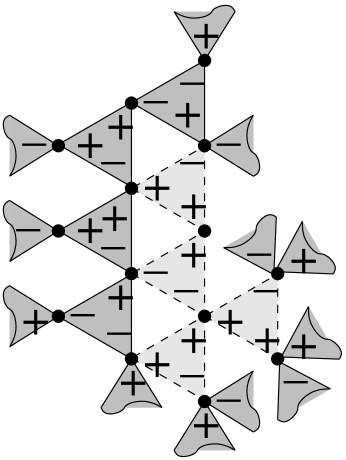
Figure 2: Example of the trimming algorithm for 3-SAT. Variables are represented graphically as vertices and clauses are represented as triangles. Signs “+” and “-” in triangles indicate whether the variable appears positively or negatively. Incomplete triangles represent connections to the remainder of the graph (not shown). Lightly shaded clauses are removed by the trimming algorithm.

As before, we use the notation $p=N^{\prime}/N$ – the probability that a randomly chosen vertex belongs to the core. The set of variables in the core is denoted as $\mathcal{C}$. We now introduce two different extensions of this set: $\mathcal{C}^{\prime}$ and $\bar{\mathcal{C}}^{\prime}$ – the minimal sets with following properties

1. $\mathcal{C}\subseteq\mathcal{C}^{\prime}$ and $\mathcal{C}\subseteq\bar{\mathcal{C}}^{\prime}$.

2. If for some clause, $K-1$ variables have a certain property, so should the remaining variable; the property being that the variable belongs to $\bar{\mathcal{C}}^{\prime}$ if it appears positively or belongs to $\mathcal{C}^{\prime}$ if it appears negatively.

We also reserve the notation $q=|\mathcal{C}^{\prime}|$ and $\bar{q}=|\bar{\mathcal{C}}^{\prime}|$. Also observe that $\mathcal{C}=\mathcal{C}^{\prime}\cap\bar{\mathcal{C}}^{\prime}$.

Fix a variable $x_{0}$. It appears in $k$ clauses positively (as $x_{0}$) and in $\bar{k}$ clauses negatively (as $\bar{x}_{0}$). The numbers $k$, $\bar{k}$ are independent random variables distributed according to a Poisson distribution with parameter $K\alpha/2$. We assume that $q$ and $\bar{q}$ for the full formula $\mathcal{F}$ are not different from $q^{\prime}$ and $\bar{q}^{\prime}$ for the formula $\mathcal{F}^{\prime}$ with variable $x_{0}$ deleted. Dropping primes we can write self-consistency equations for $q$, $\bar{q}$:

$$q = \sum_{k=0}^{\infty}\sum_{\bar{k}=1}^{\infty}\mathrm{e}^{-K\alpha\left(\frac{q+\bar{q}}{2}\right)^{K-1}}\frac{\left(\frac{K}{2}\alpha\frac{q+\bar{q}}{2}\right)^{k}}{k!}\frac{\left(\frac{K}{2}\alpha\frac{q+\bar{q}}{2}\right)^{\bar{k}}}{\bar{k}!}=1-\mathrm{e}^{-\frac{K\alpha}{2}\left(\frac{q+\bar{q}}{2}\right)^{K-1}}$$ (34)

$$\bar{q} = \sum_{k=1}^{\infty}\sum_{\bar{k}=0}^{\infty}\mathrm{e}^{-K\alpha\left(\frac{q+\bar{q}}{2}\right)^{K-1}}\frac{\left(\frac{K}{2}\alpha\frac{q+\bar{q}}{2}\right)^{k}}{k!}\frac{\left(\frac{K}{2}\alpha\frac{q+\bar{q}}{2}\right)^{\bar{k}}}{\bar{k}!}=1-\mathrm{e}^{-\frac{K\alpha}{2}\left(\frac{q+\bar{q}}{2}\right)^{K-1}}$$ (35)

Obviously $q=\bar{q}$ and a simpler equation could be written

$$q=1-\mathrm{e}^{-\frac{K\alpha}{2}q^{K-1}}.$$ (36)

Notice that this is identical to (3) with the replacement $\alpha\rightarrow\alpha/2$. As a consequence, the core appears at exactly twice the threshold for $K$-XOR-SAT (for $3$-XOR-SAT the core appears at $\alpha\approx 0.818$, and for $3$-SAT it appears at $\alpha\approx 1.636$. This threshold was obtained earlier (by a different method) in one of the first papers on lower bounds for the satisfiability transition in $3$-SAT.)

To find $p$, the sums have to be restricted to $k\geqslant 1$ and $\bar{k}\geqslant 1$ thus giving $p=q\bar{q}$. Hence

$$N^{\prime}/N=q^{2}$$ (37)

To find $M^{\prime}/N$ we need to count the average degree of the variable in the core

$$M^{\prime}/N = \frac{1}{K}\sum_{k=1}^{\infty}\sum_{\bar{k}=1}^{\infty}\left(k+\bar{k}\right)\mathrm{e}^{-K\alpha\left(\frac{q+\bar{q}}{2}\right)^{K-1}}\frac{\left(\frac{K}{2}\alpha\frac{q+\bar{q}}{2}\right)^{k}}{k!}\frac{\left(\frac{K}{2}\alpha\frac{q+\bar{q}}{2}\right)^{\bar{k}}}{\bar{k}!}$$ (38)

$$= \alpha\Big{(}\frac{q+\bar{q}}{2}\Big{)}^{K-1}\left(1-\mathrm{e}^{-\frac{K}{2}\alpha\left(\frac{q+\bar{q}}{2}\right)^{K-1}}\right).$$

Simplified, this becomes $M^{\prime}/N=\alpha q^{K}$.

III.2 Improved bound for $K$-SAT

Now that the remaining clauses are correlated, the annealed entropy for $K$-SAT is not as easily computed as for $K$-XOR-SAT. The technique parallels one used to find the annealed entropy for the ferromagnetic model. We need to find the logarithm of the number of disorders $\mathcal{N}_{J}$ and the logarithm of the number of spin-disorder combinations $\mathcal{N}_{s,J}$. In contrast to $K$-XOR-SAT, clauses acquire a type $\boldsymbol{\tau}$ – a vector, elements of which determine whether the variable in $p$-th position appears inverted or not ($\tau_{p}\in\{+,-\}$). Correspondingly, a vertex degree is now a vector $\boldsymbol{k}$ with elements $k_{\boldsymbol{\tau}}^{p}$ describing the number of appearances of a certain variable in the $p$-th position in clauses of type $\boldsymbol{\tau}$. We fix the number of variables with given $\boldsymbol{k}$: $N_{\boldsymbol{k}}^{\prime}$ (corresponding fractions are $c_{\boldsymbol{k}}=N_{\boldsymbol{k}}^{\prime}/N^{\prime}$). The number of disorders for fixed $\left\{N_{\boldsymbol{k}}^{\prime}\right\}$ and $\left\{M_{\boldsymbol{\tau}}^{\prime}\right\}$ is composed of the following factors:

1. $N^{\prime}!\big{/}\prod_{\boldsymbol{k}}N_{\boldsymbol{k}}^{\prime}!$ for the number of ways to divide the variables into classes.

2. $\prod_{p,\boldsymbol{\tau}}\left[M_{\boldsymbol{\tau}}^{\prime}!\Big{/}\prod_{\boldsymbol{k}}(k_{\boldsymbol{\tau}}^{p}!)^{N_{\boldsymbol{k}}^{\prime}}\right]$ for the number of ways to rearrange the variables among clauses.

3. $M^{\prime}!\big{/}\prod_{\boldsymbol{\tau}}M_{\boldsymbol{\tau}}^{\prime}!$ for the number of permutations of clauses of various types.

Taking the logarithm, we obtain

$$S_{J}[\{c_{\boldsymbol{k}}\}]=-N^{\prime}\sum_{\boldsymbol{k}}c_{\boldsymbol{k}}\ln\Big{[}c_{\boldsymbol{k}}\prod_{p,\boldsymbol{\tau}}k_{\boldsymbol{\tau}}^{p}!\Big{]}+K\sum_{\boldsymbol{\tau}}\left(M_{\boldsymbol{\tau}}^{\prime}\ln M_{\boldsymbol{\tau}}^{\prime}-M_{\boldsymbol{\tau}}^{\prime}\right)+M^{\prime}\ln M^{\prime}-\sum_{\boldsymbol{\tau}}M_{\boldsymbol{\tau}}^{\prime}\ln M_{\boldsymbol{\tau}}^{\prime}.$$ (39)

We must optimize over $c_{\boldsymbol{k}\bar{\boldsymbol{k}}}$ taking into account the constraint that $c_{\boldsymbol{k}}=0$ if either $|\boldsymbol{k}|=0$ or $|\bar{\boldsymbol{k}}|=0$. We also have constraints $N^{\prime}\sum_{\boldsymbol{k}}k_{\boldsymbol{\tau}}^{p}c_{\boldsymbol{k}}=M_{\boldsymbol{\tau}}^{\prime}$. Introducing dual variables and a generating function $G(x,\bar{x})=\left(e^{x}-1\right)\left(e^{\bar{x}}-1\right)$ we can write

$$S[N^{\prime},\{M_{\boldsymbol{\tau}}^{\prime}\}]=\min_{\left\{\mu_{\boldsymbol{\tau}}^{p}\right\}}\bigg{\{}\sum_{p,\boldsymbol{\tau}}M_{\boldsymbol{\tau}}^{\prime}\ln\frac{M_{\boldsymbol{\tau}}^{\prime}}{\mu_{\boldsymbol{\tau}}^{p}}+N^{\prime}\ln G(\mu,\bar{\mu})\bigg{\}}+M^{\prime}\ln M^{\prime}-\sum_{\boldsymbol{\tau}}M_{\boldsymbol{\tau}}^{\prime}\ln M_{\boldsymbol{\tau}}^{\prime}-KM^{\prime},$$ (40)

where

$$\mu = \sum_{p,\boldsymbol{\tau}}\frac{1+\tau_{p}}{2}\mu_{\boldsymbol{\tau}}^{p},$$ (41)

$$\bar{\mu} = \sum_{p,\boldsymbol{\tau}}\frac{1-\tau_{p}}{2}\mu_{\boldsymbol{\tau}}^{p}.$$ (42)

Also introducing the quantities

$$\mathcal{M} = \sum_{p,\boldsymbol{\tau}}\frac{1+\tau_{p}}{2}M_{\boldsymbol{\tau}}^{\prime},$$ (43)

$$\bar{\mathcal{M}} = \sum_{p,\boldsymbol{\tau}}\frac{1-\tau_{p}}{2}M_{\boldsymbol{\tau}}^{\prime},$$ (44)

we rewrite $S_{J}$ as

$$S_{J}[N^{\prime},\{M_{\boldsymbol{\tau}}^{\prime}\}]=\min_{\mu,\bar{\mu}}\left\{\mathcal{M}\ln\frac{\mathcal{M}}{\mu}+\bar{\mathcal{M}}\ln\frac{\bar{\mathcal{M}}}{\bar{\mu}}+N^{\prime}\ln G(\mu,\bar{\mu})\right\}+M^{\prime}\ln M^{\prime}-\sum_{\boldsymbol{\tau}}M_{\boldsymbol{\tau}}^{\prime}\ln M_{\boldsymbol{\tau}}^{\prime}.$$ (45)

For convenience we will write $G(\mu,\bar{\mu})=G_{1}(\mu)G_{1}(\bar{\mu})$. where $G_{1}(x)=e^{x}-1$. One can verify that $S_{J}$ is maximized when $M_{\boldsymbol{\tau}}^{\prime}=M^{\prime}/2^{K}$ and $\mu=\bar{\mu}=\frac{K\alpha}{2}q^{K-1}$.

Now we need to evaluate $\mathcal{N}_{s,J}$. This time the clauses are parameterized by $\boldsymbol{\tau}$ – the appearance of literals in a clause as well as $\boldsymbol{\sigma}$ – the particular assignments of variables. We fix $\left\{M_{\boldsymbol{\sigma}\boldsymbol{\tau}}^{\prime}\right\}$ as well as $\left\{N_{\boldsymbol{k}}^{\prime}\right\}$, with $\boldsymbol{k}$ being a vector with $K2^{2K}$ elements: $k_{\boldsymbol{\sigma}\boldsymbol{\tau}}^{p}$ is the number of appearances of a variable in clauses of type $(\boldsymbol{\sigma},\boldsymbol{\tau})$ in the $p$-th position. The number $\mathcal{N}_{s,J}$ can be broken into the following factors

1. $N!\big{/}\prod_{\boldsymbol{k}}N_{\boldsymbol{k}}^{\prime}!$

2. $\prod_{p,\boldsymbol{\sigma},\boldsymbol{\tau}}\left[M_{\boldsymbol{\sigma}\boldsymbol{\tau}}^{\prime}!\Big{/}\prod_{\boldsymbol{k}}\left(k_{\boldsymbol{\sigma}\boldsymbol{\tau}}^{p}!\right)^{N_{\boldsymbol{k}}^{\prime}}\right]$

3. $M^{\prime}!\big{/}\prod_{\boldsymbol{\sigma},\boldsymbol{\tau}}M_{\boldsymbol{\sigma}\boldsymbol{\tau}}^{\prime}!$

Enforcing constraints $N^{\prime}\sum_{s,\boldsymbol{k}}k_{\boldsymbol{\sigma}\boldsymbol{\tau}}^{p}c_{s,\boldsymbol{k}}=M_{\boldsymbol{\sigma}\boldsymbol{\tau}}^{\prime}$ as well as constraints on the vector $\boldsymbol{k}$, i.e. that $\sum_{p,\boldsymbol{\sigma},\boldsymbol{\tau}}\frac{1\pm\tau_{p}}{2}k_{\boldsymbol{\sigma}\boldsymbol{\tau}}^{p}\geqslant 1$ and that $c_{s,\boldsymbol{k}}=0$ if for some $p,\boldsymbol{\sigma},\boldsymbol{\tau}$ $k_{\boldsymbol{\sigma}\boldsymbol{\tau}}^{p}>0$ and $\sigma_{p}\neq s$, we are able to cast the expression for $S_{s,J}[N^{\prime},\{M_{\boldsymbol{\sigma}\boldsymbol{\tau}}^{\prime}\}]$ in a simple form

$$S_{s,J}[N^{\prime},\{M_{\boldsymbol{\sigma}\boldsymbol{\tau}}^{\prime}\}] = \min_{\mu_{\pm},\bar{\mu}_{\pm}}\Big{\{}\sum_{p,\boldsymbol{\sigma},\boldsymbol{\tau}}M_{\boldsymbol{\sigma}\boldsymbol{\tau}}^{\prime}\ln\frac{M_{\boldsymbol{\sigma}\boldsymbol{\tau}}^{\prime}}{\mu_{\boldsymbol{\sigma}\boldsymbol{\tau}}^{p}}+\ln[G(\mu_{+},\bar{\mu}_{+})+G(\mu_{-},\bar{\mu}_{-})]\Big{\}}$$ (46)

$$+M^{\prime}\ln M^{\prime}-\sum_{\boldsymbol{\sigma},\boldsymbol{\tau}}M_{\boldsymbol{\sigma}\boldsymbol{\tau}}^{\prime}\ln M_{\boldsymbol{\sigma}\boldsymbol{\tau}}^{\prime}-KM^{\prime},$$

where

$$\mu_{\pm} = \sum_{p,\boldsymbol{\sigma},\boldsymbol{\tau}}\frac{1+\tau_{p}}{2}\frac{1\pm\sigma_{p}}{2}\mu_{\boldsymbol{\sigma}\boldsymbol{\tau}}^{p},$$ (47)

$$\bar{\mu}_{\pm} = \sum_{p,\boldsymbol{\sigma},\boldsymbol{\tau}}\frac{1-\tau_{p}}{2}\frac{1\pm\sigma_{p}}{2}\mu_{\boldsymbol{\sigma}\boldsymbol{\tau}}^{p}.$$ (48)

Also introducing

$$\mathcal{M}_{\pm} = \sum_{p,\boldsymbol{\sigma},\boldsymbol{\tau}}\frac{1+\tau_{p}}{2}\frac{1\pm\sigma_{p}}{2}M_{\boldsymbol{\sigma}\boldsymbol{\tau}}^{\prime},$$ (49)

$$\bar{\mathcal{M}}_{\pm} = \sum_{p,\boldsymbol{\sigma},\boldsymbol{\tau}}\frac{1-\tau_{p}}{2}\frac{1\pm\sigma_{p}}{2}M_{\boldsymbol{\sigma}\boldsymbol{\tau}}^{\prime},$$ (50)

we can rewrite the first part of $S_{s,J}$ as

$$S_{s,J}^{(1)}[N^{\prime},\{M_{\boldsymbol{\sigma}\boldsymbol{\tau}}^{\prime}\}]=\min_{\mu_{\pm},\bar{\mu}_{\pm}}\Big{\{} \mathcal{M}_{+}\ln\frac{\mathcal{M}_{+}}{\mu_{+}}+\mathcal{M}_{-}\ln\frac{\mathcal{M}_{-}}{\mu_{-}}+\bar{\mathcal{M}}_{+}\ln\frac{\bar{\mathcal{M}}_{+}}{\bar{\mu}_{+}}+\bar{\mathcal{M}}_{-}\ln\frac{\bar{\mathcal{M}}_{-}}{\bar{\mu}_{-}}$$ (51)

$$+N^{\prime}\ln[G(\mu_{+},\bar{\mu}_{+})+G(\mu_{-},\bar{\mu}_{-})]\Big{\}}$$

Next, we optimize the expression $M^{\prime}\ln M^{\prime}-\sum_{\boldsymbol{\sigma},\boldsymbol{\tau}}M_{\boldsymbol{\sigma}\boldsymbol{\tau}}^{\prime}\ln M_{\boldsymbol{\sigma}\boldsymbol{\tau}}^{\prime}$ subject to fixed $\mathcal{M}_{+}$, $\mathcal{M}_{-}$, $\bar{\mathcal{M}}_{+}$, $\bar{\mathcal{M}}_{-}$. Introducing dual variables $-h,-h^{\prime},-h^{\prime\prime}$ coupled to $\mathcal{M}_{+}-\mathcal{M}_{-}-\bar{\mathcal{M}}_{+}+\bar{\mathcal{M}}_{-}$, $\mathcal{M}_{+}-\mathcal{M}_{-}+\bar{\mathcal{M}}_{+}-\bar{\mathcal{M}}_{-}$ and $\mathcal{M}_{+}+\mathcal{M}_{-}-\bar{\mathcal{M}}_{+}-\bar{\mathcal{M}}_{-}$ respectively, the optimized expression becomes

$$S_{s,J}^{(2)}[N^{\prime},\mathbf{\mathcal{M}}] =\min_{h,h^{\prime},h^{\prime\prime}}\Big{\{}-h(\mathcal{M}_{+}-\mathcal{M}_{-}-\bar{\mathcal{M}}_{+}+\bar{\mathcal{M}}_{-})-h^{\prime}(\mathcal{M}_{+}-\mathcal{M}_{-}+\bar{\mathcal{M}}_{+}-\bar{\mathcal{M}}_{-})$$

$$-h^{\prime\prime}(\mathcal{M}_{+}+\mathcal{M}_{-}-\bar{\mathcal{M}}_{+}-\bar{\mathcal{M}}_{-})-M^{\prime}\ln\sum_{\boldsymbol{\sigma}\boldsymbol{\tau}}\epsilon_{\boldsymbol{\sigma}\boldsymbol{\tau}}\mathrm{e}^{\left(\sum_{p}\sigma_{p}\tau_{p}\right)h+\left(\sum_{p}\sigma_{p}\right)h^{\prime}+\left(\sum_{p}\tau_{p}\right)h^{\prime\prime}}\Big{\}}$$

where $\epsilon_{\boldsymbol{\sigma}\boldsymbol{\tau}}\in\{0,1\}$ determines whether the clause is permitted. For the case of $K$-SAT we only prohibit combinations $\prod_{p}\frac{1+\sigma_{p}\tau_{p}}{2}=1$. We can express $\mathcal{M}_{+},\mathcal{M}_{-},\bar{\mathcal{M}}_{+},\bar{\mathcal{M}}_{-}$ in terms of $h,h^{\prime}$ and $h^{\prime\prime}$ and substitute into (51). Consequently, maximization over $h,h^{\prime},h^{\prime\prime}$ will be performed. It can be shown that the maximum necessarily corresponds to $h^{\prime}=h^{\prime\prime}=0$ leading to further simplifications:

$$\sum_{\boldsymbol{\sigma},\boldsymbol{\tau}}\epsilon_{\boldsymbol{\sigma}\boldsymbol{\tau}}\mathrm{e}^{\left(\sum_{p}\sigma_{p}\tau_{p}\right)h}=(2\cosh h)^{K}-\mathrm{e}^{Kh},$$ (53)

and we can show that $\bar{\mathcal{M}}_{+}=\mathcal{M}_{-}$ and $\bar{\mathcal{M}}_{-}=\mathcal{M}_{+}$. (As a result $\bar{\mu}_{+}=\mu_{-}$ and $\bar{\mu}_{-}=\mu_{+}$).

$$S_{\textrm{ann}}=\max_{h}\Big{\{} +\min_{\mu}\big{\{}2\mathcal{M}_{+}\ln\frac{2\mathcal{M}_{+}}{\mu}+N^{\prime}\ln G_{1}(\mu)\big{\}}+\min_{\mu}\big{\{}2\mathcal{M}_{-}\ln\frac{2\mathcal{M}_{-}}{\mu}+N^{\prime}\ln G_{1}(\mu)\big{\}}$$ (54)

$$-2\min_{\mu}\left\{\frac{KM^{\prime}}{2}\ln\frac{KM^{\prime}/2}{\mu}+N^{\prime}\ln G_{1}(\mu)\right\}+N^{\prime}\ln 2-KM^{\prime}\ln 2$$

$$-h(2\mathcal{M}_{+}-2\mathcal{M}_{-})+M^{\prime}\ln\left[(2\cosh h)^{K}-\mathrm{e}^{Kh}\right]\Big{\}},$$

where $\mathcal{M}_{\pm}$ are the functions of $h$:

$$2\mathcal{M}_{\pm}=\frac{1}{2}KM^{\prime}\pm\frac{1}{2}\frac{\mathrm{d}}{\mathrm{d}h}\ln\sum_{\boldsymbol{\sigma}\boldsymbol{\tau}}\epsilon_{\boldsymbol{\sigma}\boldsymbol{\tau}}\mathrm{e}^{\left(\sum_{p}\sigma_{p}\tau_{p}\right)h},$$ (55)

or, substituting $\epsilon_{\boldsymbol{\sigma}\boldsymbol{\tau}}$ for $K$-SAT

$$2\mathcal{M}_{+} = KM^{\prime}\mathrm{e}^{h}\frac{(2\cosh h)^{K-1}-\mathrm{e}^{(K-1)h}}{(2\cosh h)^{K}-\mathrm{e}^{Kh}},$$ (56)

$$2\mathcal{M}_{-} = KM^{\prime}\mathrm{e}^{-h}\frac{(2\cosh h)^{K-1}}{(2\cosh h)^{K}-\mathrm{e}^{Kh}}.$$ (57)

We also verify that the maximum of the complete expression corresponds to $h=0$. As a result

$$S_{\textrm{ann}} = \min_{\mu}\left\{2\mathcal{M}_{+}\ln\frac{2\mathcal{M}_{+}}{\mu}+N^{\prime}\ln G_{1}(\mu)\right\}+\min_{\mu}\left\{2\mathcal{M}_{-}\ln\frac{2\mathcal{M}_{-}}{\mu}+N^{\prime}\ln G_{1}(\mu)\right\}$$ (58)

$$-2\min_{\mu}\left\{\frac{KM^{\prime}}{2}\ln\frac{KM^{\prime}/2}{\mu}+N^{\prime}\ln G_{1}(\mu)\right\}+N^{\prime}\ln 2+M^{\prime}\ln\left[1-2^{-K}\right]$$

Solving $S_{\textrm{ann}}=0$ translates into an upper bound for $K=3$ of $\alpha_{u}^{\prime}\approx 5.189$ – a rather insignificant improvement over straightforward annealing approximation.

IV Positive $1$-in-$K$-SAT model

In this model, we have a set of clauses, each clause involving $K$ variables that can take values $0$ or $1$. A clause is satisfied if the sum of values of variables is exactly $1$. A formula is satisfied if all the clauses that constitute it are satisfied. A related problem was considered in farhi in the context of the quantum adiabatic algorithm, which served as the main motivation for present analysis. For a randomly generated formula, the satisfiability transition occurs for some critical clause-to-variable ratio $\alpha=M/N$. The easiest upper bound is obtained using the straightforward annealing approximation. For the logarithm of the expected number of solutions we obtain

$$\ln\mathbbm{E}[\mathcal{N}]=\max_{m}\bigg{\{}-N\Big{(}\frac{1+m}{2}\ln\frac{1+m}{2}+\frac{1-m}{2}\ln\frac{1-m}{2}\Big{)}+M\ln\Big{[}3\frac{1-m}{2}\left(\frac{1+m}{2}\right)^{2}\Big{]}\bigg{\}},$$ (59)

where we identified $m=1$ with having all variables assigned a value of $0$, $m=-1$ with having all variables set to $1$, and intermediate values of $m$ being the appropriate mixture.

The annealed entropy becomes $0$ at the critical threshold $\alpha_{u}\approx 0.805$. We now seek to improve upon this simplistic approximation.

IV.1 Core for positive $1$-in-$K$-SAT

The structure of the core for positive $1$-in-$K$-SAT is more complex than what we have seen before. As before variables of degree $0$ are eliminated. Similarly variables of degree $1$ are removed, although we are no longer justified in removing the clause in which variable appears. Instead, the corresponding $K$-clause has to be replaced with a $(K-1)$-clause. The latter is deemed to be satisfied if the sum of variables in it is either $0$ or $1$. Then the remaining variable could always be set to either $0$ or $1$ so that the sum of all $K$ variables is exactly $1$. Similarly, if any variable has degree $1$ and appears in a $(K-1)$-clause, the latter can be converted to a $(K-2)$-clause and so on. For all clauses of length less than $K$, the criterion for satisfiability is that the sum of variables be either $0$ or $1$. Finally, we identify variables that appear only in $2$ clauses. Setting any such variable to $0$ will satisfy all $2$-clauses. Thus, such variables and clauses in which they appear can be eliminated. This process continues until we are left with a subformula where the degree of each variable is $\geqslant 2$ and no variable appears only in $2$-clauses (see Fig. 3).

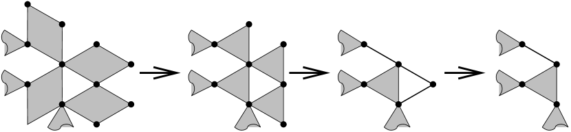
Figure 3: Example of the trimming algorithm for 1-in-4-SAT. Variables are represented graphically as vertices and 4-, 3- and 2-clauses are represented as rhombi, triangles and edges correspondingly. Incomplete polygons represent connections to the remainder of the graph. The figure depicts evolution of part of the graph under the trimming algorithm.

For any fixed $N^{\prime}$ and a set of $\{M_{k}^{\prime}\}$ (with $k=2,\ldots,K$) – the number of clauses of length $k$ – all subformulae that satisfy aforementioned constraints are equally probable. The values $N^{\prime}/N$ and $\{M_{k}^{\prime}/N\}$ are self-averaging and their means will be computed shortly.

As before, we introduce the following notation. $\mathcal{C}$ denotes the set of variables that belong to the core. In addition to $\mathcal{C}$ we introduce sets $\mathcal{C}_{2}^{\prime}$ and $\mathcal{C}^{\prime}$. The sets shall have the following properties:

1. $\mathcal{C}\subseteq\mathcal{C}^{\prime}\subseteq\mathcal{C}_{2}^{\prime}$.

2. If $2$ variables in some clause belong to $\mathcal{C}^{\prime}$, then all variables in that clause belong to $\mathcal{C}^{\prime}$.

3. If $1$ variable in some clause belongs to $\mathcal{C}_{2}^{\prime}$, then all variables in that clause belong to $\mathcal{C}_{2}^{\prime}$.

We reserve the notation $p=|\mathcal{C}|/N$, $q=|\mathcal{C}^{\prime}|/N$ and $q_{2}=|\mathcal{C}_{2}^{\prime}|/N$. As before, we single out a single variable $x_{0}$ and study the probability that the variable belongs to classes $\mathcal{C}$, $\mathcal{C}^{\prime}$ or $\mathcal{C}_{2}^{\prime}$. The number of clauses in which the variable appears is Poisson with parameter $K\alpha$. The variable $x_{0}$ is in $\mathcal{C}^{\prime}$ if for at least one clause in which $x_{0}$ appears at least two variables among the $K-1$ remaining variables belong to $\mathcal{C}_{2}^{\prime}$.

$$q=1-\exp\left[-K\alpha\left(1-(1-q_{2})^{K-1}-(K-1)q_{2}(1-q_{2})^{K-2}\right)\right],$$ (60)

where we have used the fact that the probability that among randomly chosen $K-1$ variables the probability that at least two belong to $\mathcal{C}_{2}^{\prime}$ is $1-(1-q_{2})^{K-1}-(K-1)q_{2}(1-q_{2})^{K-2}$.

The variable $x_{0}$ is in $\mathcal{C}_{2}^{\prime}$ if for at least one clause, at least one variable among the other $(K-1)$ variables belongs to $\mathcal{C}^{\prime}$ or at least two variables belong to $\mathcal{C}_{2}^{\prime}$. The probability of that is $1-(1-q_{2})^{K-1}-(K-1)(q_{2}-q)(1-q)^{K-2}$. The second self-consistency equation is thus

$$q_{2}=1-\exp\left[-K\alpha\left(1-(1-q_{2})^{K-1}-(K-1)(q_{2}-q)(1-q_{2})^{K-2}\right)\right].$$ (61)

Consider clauses in which the variable $x_{0}$ appears. Let us call those clauses in which at least two variables appear in $\mathcal{C}_{2}^{\prime}$ type-$1$ clauses, and those clauses in which one variable belongs to $\mathcal{C}^{\prime}$ – type-$2$ clauses. Variable $x_{0}$ is in $\mathcal{C}$ if it appears in two or more type-$1$ or type-$2$ clauses, and at least one type-$1$ clause. Therefore, we should have

$$p=1-\mathrm{e}^{-K\alpha p_{1}}-K\alpha p_{1}\mathrm{e}^{-K\alpha p_{2}},$$ (62)

where

$$p_{1} = 1-(1-q_{2})^{K-1}-(K-1)q_{2}(1-q_{2})^{K-2},$$ (63)

$$p_{2} = 1-(1-q_{2})^{K-1}-(K-1)(q_{2}-q)(1-q_{2})^{K-2}.$$ (64)

To find the number of $k$-clauses in the core $M_{k}^{\prime}$, compute the average $k$-degree of variable $x_{0}$, i.e. the number of $k$-clauses in which it appears. We readily obtain the following formulae:

$$M_{2}^{\prime}/N = \binom{K}{2}\alpha q^{2}(1-q_{2})^{K-2},$$ (65)

$$M_{k}^{\prime}/N = \binom{K}{k}\alpha q_{2}^{k}(1-q_{2})^{K-k},\textrm{for }k\geqslant 3.$$ (66)

IV.2 Improved bound for positive $1$-in-$K$-SAT

As before, we compute $\mathcal{N}_{J}$ – the number of disorders, subject to fixed $N^{\prime}$ and $\{M_{k}^{\prime}\}$, under the condition that each variable has a degree of at least two, and that no variable appears in $2$-clauses exclusively. Introduce a vector of length $K-1$ of vertex degrees $(k_{2},\ldots,k_{K})$, with elements being the number of $k$-clauses in which the variable appears. We prohibit vertices with$\sum_{i=3}^{K}k_{i}=0$ or $\sum_{i=2}^{K}k_{i}=1$. The corresponding generating function

$$G(\boldsymbol{x})=\sum_{\{k_{i}\}}^{\prime}\prod_{i=2}^{K}\frac{(x_{i})^{k_{i}}}{k_{i}!}=\mathrm{e}^{\sum_{i=2}^{K}x_{i}}-\mathrm{e}^{x_{2}}-\sum_{i=3}^{K}x_{i}.$$ (67)

It is convenient to write $G(\boldsymbol{x})=G_{2}\left(x_{2},\sum_{k=3}^{K}x_{k}\right)$, where $G_{2}(x,y)=\mathrm{e}^{x+y}-e^{x}-y$.

We proceed to counting the number of disorders with fixed $N^{\prime}$ and $\{M_{k}^{\prime}\}$. It is convenient to introduce the quantities $N_{\boldsymbol{k}_{2}\ldots\boldsymbol{k}_{K}}^{\prime}$ that count the number of vertices; indices $k_{i}^{p}$ being the number of appearances in $p$-th position in a clause of length $i$. Starting from

$$S_{J}[c_{\boldsymbol{k}_{2}\ldots\boldsymbol{k}_{K}}]=-N^{\prime}\sum_{\boldsymbol{k}_{2}\ldots\boldsymbol{k}_{K}}c_{\boldsymbol{k}_{2}\ldots\boldsymbol{k}_{K}}\ln\Big{[}c_{\boldsymbol{k}_{2}\ldots\boldsymbol{k}_{K}}\prod_{i,p}k_{i}^{p}!\Big{]}+\sum_{k=2}^{K}k(M_{k}^{\prime}\ln M_{k}^{\prime}-M_{k}^{\prime})$$ (68)

and optimizing over $c_{\boldsymbol{k}_{2}\ldots\boldsymbol{k}_{K}}$ subject to constraints on degrees as well as the set of constraints

$$N^{\prime}\sum_{\boldsymbol{k}_{2}\ldots\boldsymbol{k}_{K}}k_{i}^{p}c_{\boldsymbol{k}_{2}\ldots\boldsymbol{k}_{K}}=M_{i}^{\prime}$$ (69)

we obtain

$$S_{J}[N^{\prime},\{M_{k}^{\prime}\}]=\min_{\{\mu_{k}\}}\Big{\{}\sum_{k=2}^{K}kM_{k}^{\prime}\ln\frac{kM_{k}^{\prime}}{\mu_{k}}+N^{\prime}\ln G(\{\mu_{k}\})\Big{\}}-\sum_{k=2}^{K}kM_{k}^{\prime}$$ (70)

Using the relation $G(\{\mu_{k}\})=G_{2}\big{(}\mu_{2},\sum_{k=3}^{K}\mu_{k}\big{)}$ rewrite

$$S_{J}[N^{\prime},\{M_{k}^{\prime}\}] = \min_{\mu_{2},\mu}\bigg{\{}2M_{2}^{\prime}\ln\frac{2M_{2}^{\prime}}{\mu_{2}}+\Big{(}\sum^{K}_{k=3}kM_{k}^{\prime}\Big{)}\ln\frac{\sum_{k=3}^{K}kM_{k}^{\prime}}{\mu}+N^{\prime}\ln G_{2}(\mu_{2},\mu)\bigg{\}}$$ (71)

$$-\sum_{k=2}^{K}kM_{k}^{\prime}.$$

Now, compute the total number of disorders and variable assignments compatible with them. Now the clauses of each length have to be subdivided into types $\boldsymbol{\sigma}_{2}$ through $\boldsymbol{\sigma}_{K}$, according to the variable assignments in the corresponding clause. We arrange variables into classes according to their value $s\in\{+,-\}$ and a vector $(\boldsymbol{k}_{2},\ldots,\boldsymbol{k}_{K})$, with $k_{\boldsymbol{\sigma}_{i}}^{p}$ being the number of appearances of a variable in a clause of length $i$ and type $\boldsymbol{\sigma}_{i}$ in $p$-th position. The number $\mathcal{N}_{s,J}$ is given as a product of three factors

1. $N^{\prime}!\big{/}\prod_{s,\boldsymbol{k}_{2}\ldots\boldsymbol{k}_{K}}N_{s,\boldsymbol{k}_{2}\ldots\boldsymbol{k}_{K}}^{\prime}!$ for the number of ways to rearrange the variables into classes

2. $\prod_{i=2}^{K}\prod_{p}\prod_{\boldsymbol{\sigma}_{i}}\left[M_{\boldsymbol{\sigma}_{i}}^{\prime}!\Big{/}\prod_{s,\boldsymbol{k}_{2}\ldots\boldsymbol{k}_{K}}(k_{\boldsymbol{\sigma}_{i}}^{p}!)^{N_{s,\boldsymbol{k}_{2}\ldots\boldsymbol{k}_{K}}}\right]$ for the number of ways to rearrange variables inside the clauses.

3. $\prod_{i=2}^{K}\left[M_{i}^{\prime}!\big{/}\sum_{\boldsymbol{\sigma}_{i}}M_{\boldsymbol{\sigma}_{i}}^{\prime}!\right]$ for the number of ways to rearrange clauses.

For the entropy we obtain

$$S_{s,J}[c_{s,\boldsymbol{k}_{2}\ldots\boldsymbol{k}_{K}}] = -N^{\prime}\sum_{s,\boldsymbol{k}_{2}\ldots\boldsymbol{k}_{K}}c_{s,\boldsymbol{k}_{2}\ldots\boldsymbol{k}_{K}}\ln\Big{[}c_{s,\boldsymbol{k}_{2}\ldots\boldsymbol{k}_{K}}\prod_{i,\boldsymbol{\sigma}_{\boldsymbol{i}},p}k_{\boldsymbol{\sigma}_{i}}^{p}!\Big{]}+\sum_{i,\boldsymbol{\sigma}_{i}}i\left(M_{\boldsymbol{\sigma}_{i}}^{\prime}\ln M_{\boldsymbol{\sigma}_{i}}^{\prime}-M_{\boldsymbol{\sigma}_{i}}^{\prime}\right)$$ (72)

$$+\sum_{i}M_{i}^{\prime}\ln M_{i}^{\prime}-\sum_{i,\boldsymbol{\sigma}_{i}}M_{\boldsymbol{\sigma}_{i}}^{\prime}\ln M_{\boldsymbol{\sigma}_{i}}^{\prime}.$$

We must note the constraints

$$N^{\prime}\sum_{\boldsymbol{k}_{2}\ldots\boldsymbol{k}_{K}}k_{\boldsymbol{\sigma}_{i}}^{p}=M_{\boldsymbol{\sigma}_{i}}^{p}$$ (73)

as well as constraints on variable value ($k_{\boldsymbol{\sigma}_{i}}^{p}\neq 0\Rightarrow\sigma_{i}^{p}=s$) and on the degrees of the variables ($\sum_{i=3}^{K}|\boldsymbol{k}_{i}|\geqslant 1$ and $\sum_{i=2}^{K}|\boldsymbol{k}_{i}|\geqslant 2$). With the aid of the generating function and the dual variables we can write

$$S_{s,J}[N^{\prime},\{M_{k}\}] = \min_{\{\mu_{\boldsymbol{\sigma}_{k}}^{p}\}}\bigg{\{}\sum_{k,\boldsymbol{\sigma}_{k},p}M_{\boldsymbol{\sigma}_{k}}^{\prime}\ln\frac{M_{\boldsymbol{\sigma}_{k}}^{\prime}}{\mu_{\boldsymbol{\sigma}_{k}}^{p}}+N^{\prime}\ln\left[G\left(\left\{\mu_{k+}\right\}\right)+G\left(\left\{\mu_{k-}\right\}\right)\right]\bigg{\}}$$ (74)

$$+\sum_{k}M_{k}^{\prime}\ln M_{k}^{\prime}-\sum_{k,\boldsymbol{\sigma}_{k}}M_{\boldsymbol{\sigma}_{k}}^{\prime}\ln M_{\boldsymbol{\sigma}_{k}}^{\prime}-\sum_{k}kM_{k}^{\prime},$$

where we have written $\mu_{k\pm}=\sum_{p,\boldsymbol{\sigma}_{k}}\frac{1+\sigma_{k}^{p}}{2}\mu_{\boldsymbol{\sigma}_{k}}^{p}$. Also, introducing $\mathcal{M}_{k\pm}=\sum_{p,\boldsymbol{\sigma}_{k}}\frac{1+\sigma_{k}^{p}}{2}M_{\boldsymbol{\sigma}_{k}}^{\prime}$ the first subexpression can be simplified to

$$S_{s,J}^{(1)}[N^{\prime},\mathbf{\mathcal{M}}]=\min_{\left\{\mu_{k}^{\pm}\right\}}\bigg{\{}\sum_{k}\Big{(}\mathcal{M}_{k+}\ln\frac{\mathcal{M}_{k+}}{\mu_{k+}}+\mathcal{M}_{k-}\ln\frac{\mathcal{M}_{k-}}{\mu_{k-}}\Big{)}+N^{\prime}\ln\left[G\left(\left\{\mu_{k+}\right\}\right)+G\left(\left\{\mu_{k-}\right\}\right)\right]\bigg{\}},$$ (75)

and using $G_{2}$ can be rewritten as

$$S_{s,J}^{(1)}[N^{\prime},\mathbf{\mathcal{M}}]= \min_{\mu_{2\pm},\mu_{\pm}}\bigg{\{}\mathcal{M}_{2+}\ln\frac{\mathcal{M}_{2+}}{\mu_{2+}}+\mathcal{M}_{2+}\ln\frac{\mathcal{M}_{2-}}{\mu_{2-}}+\Big{(}\sum_{k=3}^{K}\mathcal{M}_{k+}\Big{)}\ln\frac{\sum_{k=3}^{K}\mathcal{M}_{k+}}{\mu_{+}}$$ (76)

$$+\Big{(}\sum_{k=3}^{K}\mathcal{M}_{k-}\Big{)}\ln\frac{\sum_{k=3}^{K}\mathcal{M}_{k-}}{\mu_{-}}+\ln\left[G_{2}\left(\mu_{2+},\mu_{-}\right)+G_{2}\left(\mu_{2-},\mu_{-}\right)\right]\bigg{\}}$$

In correspondence with the different treatment afforded to $2$-clauses and $k$-clauses for $k\geqslant 3$, we introduce two fields $-h_{2}$ and $-h$ coupled to $\mathcal{M}_{2+}-\mathcal{M}_{2-}$ and $\sum_{k=3}^{K}\left(\mathcal{M}_{k+}-\mathcal{M}_{k-}\right)$ correspondingly. The dual of second part of $S_{s,J}$ is

$$\tilde{S}_{s,J}^{(2)}[h_{2},h]=\min_{\left\{M_{\boldsymbol{\sigma}_{k}}^{\prime}\right\}}\bigg{\{} -h_{2}\left(\mathcal{M}_{2+}-\mathcal{M}_{2-}\right)-h\sum_{k=3}^{K}\left(\mathcal{M}_{k+}-\mathcal{M}_{k-}\right)$$ (77)

$$-\sum_{k=2}^{K}\Big{(}M_{k}^{\prime}\ln M_{k}^{\prime}-\sum_{\boldsymbol{\sigma}_{k}}M_{\boldsymbol{\sigma}_{k}}^{\prime}\ln M_{\boldsymbol{\sigma}_{k}}^{\prime}\Big{)}\bigg{\}}.$$

Note that for $k=K$ only $\sum_{p}\sigma_{K}^{p}=K-1$ is allowed, while for $k<K$, $\sum_{p}\sigma_{k}^{p}=K$ and $\sum_{p}\sigma_{k}^{p}=K-1$ are both allowed. After proper minimizations we obtain

$$\tilde{S}_{s,J}^{(2)}[h_{2},h]=M_{2}^{\prime}\ln\left(2+\mathrm{e}^{h_{2}}\right)+\sum_{k=3}^{K-1}M_{k}^{\prime}\ln\left(k\mathrm{e}^{(k-1)h}+\mathrm{e}^{kh}\right)+M_{K}^{\prime}\ln\left(K\mathrm{e}^{Kh}\right).$$ (78)

We can express $\left\{M_{k}^{\pm}\right\}$ in terms of $h_{2}$ and $h$ via

$$\mathcal{M}_{2\pm} = M_{2}^{\prime}\pm\frac{1}{2}\frac{\partial}{\partial h_{2}}\tilde{S}_{s,J}^{(2)}[h_{2},h],$$ (79)

$$\sum_{k=3}^{K}\mathcal{M}_{k\pm} = \sum_{k=3}^{K}kM_{k}^{\prime}\pm\frac{1}{2}\frac{\partial}{\partial h}\tilde{S}_{s,J}^{(2)}[h_{2},h].$$ (80)

The entire expression for the annealed entropy is then written as

$$\tilde{S}_{\textrm{ann}}[h_{2},h] = \min_{\mu_{2\pm},\mu_{\pm}}\Bigg{\{}\mathcal{M}_{2+}\ln\frac{\mathcal{M}_{2+}}{\mu_{2+}}+\mathcal{M}_{2+}\ln\frac{\mathcal{M}_{2-}}{\mu_{2-}}+\Big{(}\sum_{k=3}^{K}\mathcal{M}_{k+}\Big{)}\ln\frac{\sum_{k=3}^{K}\mathcal{M}_{k+}}{\mu_{+}}$$ (81)

$$+\Big{(}\sum_{k=3}^{K}\mathcal{M}_{k-}\Big{)}\ln\frac{\sum_{k=3}^{K}\mathcal{M}_{k-}}{\mu_{-}}+\ln\left[G_{2}\left(\mu_{2+},\mu_{-}\right)+G_{2}\left(\mu_{2-},\mu_{-}\right)\right]\Bigg{\}}$$

$$-\min_{\mu_{2},\mu}\bigg{\{}2M_{2}^{\prime}\ln\frac{2M_{2}^{\prime}}{\mu_{2}}+\Big{(}\sum^{K}_{k=3}kM_{k}^{\prime}\Big{)}\ln\frac{\sum_{k=3}^{K}kM_{k}^{\prime}}{\mu}+N^{\prime}\ln G_{2}(\mu_{2},\mu)\bigg{\}}$$

$$-h_{2}(\mathcal{M}_{2+}-\mathcal{M}_{2-})-h\sum_{k=3}^{K}(\mathcal{M}_{k+}-\mathcal{M}_{k-})$$

$$+M_{2}^{\prime}\ln(2+\mathrm{e}^{h_{2}})+\sum_{k=3}^{K-1}M_{k}^{\prime}\ln\left(k\mathrm{e}^{(k-1)h}+\mathrm{e}^{kh}\right)+M_{K}^{\prime}\ln\left(K\mathrm{e}^{Kh}\right)$$

Maximization over $h_{2},h$ and solving $S_{\textrm{ann}}=0$ gives an upper bound for the satisfiability transition. For $K=3$ we obtain $\alpha_{u}\approx 0.644$. This compares favorably to $\alpha_{c}\approx 0.625$ observed in simulations and beats the previous best upper bound of $\alpha_{u}\approx 0.727$ moore .

V Simulation results

In this section we present experimental results on random positive 1-in-3-SAT instances. Using the Davis-Putnam (DP) algorithm (see Appendix A) we study the crossover point and the computation complexity. We also identify experimentally the position of the phase transition.

V.1 The Crossover Point

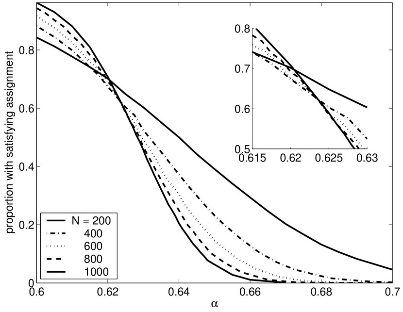
Figure 4: Proportion of problem instances with a satisfying assignment

The major feature of a phase transition in a satisfiability problem is the presence of a threshold in $\alpha$, below which almost all random problem instances are solvable, and above which almost no random problem instances are. Figure 4 shows a plot of the proportion of random problem instances that have a satisfying assignment, versus $\alpha$, for various values of $N$. The proportions are based on running the DP algorithm on 50,000 random problem instances for each value of $N$ and $\alpha$. The expected features are present. The sharpness of the phase transition increases with $N$, and the point at which the curve crosses the line where the proportion of instances with a satisfying assignment equals $0.5$ decreases with $N$.

Experimentally the crossover point is at $\alpha_{c}\approx 0.625$, slightly lower than the upper bound of $\alpha_{u}\approx 0.644$ computed in section IV. In figure 5 (lower curve) we plot the value of $\alpha$ for which 50% of the problem instances were satisfiable as a function of the number of bits. The curve appears to have an asymptote around $\alpha_{c}\approx 0.625$.

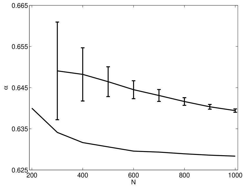
Figure 5: Top curve: plot of the maximum complexity of the DP algorithm. Lower curve: the position of the crossing point of proportion with satisfying assignment = 0.5

V.2 Complexity of the Davis-Putnam Algorithm

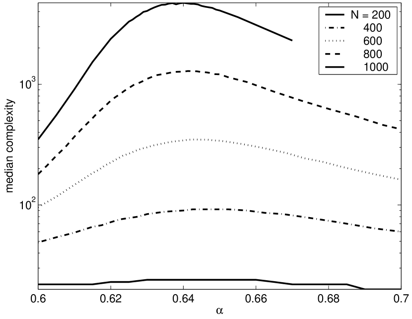
Figure 6: Computational complexity of DP

Figure 6 shows plots of the median complexity of the Davis-Putnam (DP) algorithm (complexity is defined as the number of calls to the function Find_Model displayed in Table 1). The median was taken over 50,000 random problem instances. As expected, because the DP algorithm is complete, its performance scales exponentially with problem size, $N$. Note also that the value of $\alpha$ for which the maximum complexity occurs is above $\alpha_{c}$, and slowly reduces as $N$ increases. In figure 5 (upper curve) we plot the position of the maximum complexity and its uncertainty. we note that for the range of values of $N$ considered, it does not appear to have converged to an asymptote, but the curve does not appear to contradict our earlier result of $\alpha_{c}\approx 0.625$.

Fitting an exponential law to the peak complexity gives $C=6.13\exp(0.0067\times N)$, a very slow rate of increase – an order of magnitude slower than reported results on the complexity of DP applied to 3-SAT ksat2 .

VI Summary

In this paper we have proposed a new method for analyzing subgraphs (subformulae) of the random graph (formula) subject to simple geometric constraints. For every constraint satisfaction problem one can identify a core – a subformula that is satisfiable if and only if the original formula was satisfiable. In fact simplifying the original formula is typically a first step before applying general-purpose algorithms such as the Davis-Putnam routine or simulated annealing, and the best algorithms use it. This may become an essential tool for the analysis of “smart” algorithms that perform transformations on the instance of the problem or even on intermediate steps. We have also applied the methods used in the present paper for the approximate analysis of the quantum adiabatic algorithm for positive $1$-in-$K$-SAT problem self .

We have also tried to estimate the satisfiability transition from the above for three problems: $K$-XOR-SAT, $K$-SAT and Positive $1$-in-$K$-SAT. The results for $K=3$ are as follows: $\alpha_{u}\approx 0.918$ for $K$-XOR-SAT (exact), $\alpha_{u}\approx 5.189$ for $K$-SAT (vs. $\alpha_{c}\approx 4.2$ experimentally) and $\alpha_{u}\approx 0.644$ for positive $1$-in-$K$-SAT (vs. $\alpha_{c}\approx 0.625$ experimentally).

The bound for $K$-SAT was an insignificant improvement over the annealing approximation despite deleting irrelevant clauses that contribute to the entropy. Results for $K$-XOR-SAT and $1$-in-$K$-SAT were quite good. Note that random $1$-in-$K$-SAT (where variables may appear in clauses either positively or negatively with probability $1/2$, akin to $K$-SAT) is quite simple. The satisfiability transition coincides with percolation, and algorithms solve the problem very efficiently in the satisfiable phase. A precise way to state this is that the dynamical transition coincides with the satisfiability transition, shrinking the difficult region. This is not the case for positive $1$-in-$K$-SAT that we consider, where most likely $\alpha_{d}<\alpha_{c}$.

That the annealing approximation for the simplified formula fails to predict the correct transition suggests that a large number of solutions remains up to the satisfiability threshold. In all likelihood these individual solutions are well-separated, which may explain the poor performance of algorithms. We conjecture that random instances of positive $1$-in-$K$-SAT are significantly simpler to solve than those of $K$-SAT. This view is partly supported by simulations. Also observe that the answer for $K$-XOR-SAT – a polynomial problem – is exact.

VII Acknowledgments

This work was supported in part by the National Security Agency (NSA) and Advanced Research and Development Activity (ARDA) under Army Research Office (ARO) contract number ARDA-QC-P004-J132-Y03/LPS-FY2003, we also want to acknowledge the partial support of NASA CICT/IS program.

Appendix A The Davis-Putnam Algorithm

The Davis-Putnam (DP) algorithm davis60 , or a variation, is regarded as the most efficient complete algorithm for satisfiability problems. An outline of the DP algorithm is given in table 1 ksat2 . The version we used varies from this outline in one major respect. We perform a sort of the variables before the first call to Find_Model, sorting on the number of clauses which use the variable. This was found to produce, on average, a very large speed-up in the algorithm’s execution.

The unit_propagate step of the algorithm is also extremely efficient for the $1$-in-$K$-SAT problem. Once one variable in a clause is set to $1$, the value of the other two variables is fixed, and extensive propagation often occurs. Also, because a single variable in a clause being set to $1$ determines the other two variables in the clause, we call Find_Model( theory AND x ) first.

Table 1: Outline of the Davis-Putnam Algorithm

Find_Model( theory )
  unit_propagate( theory );
  if contradiction discovered return(false);
  else if all variables are valued return(true);
  else {
    x = some unvalued variable;
    return( Find_Model( theory AND x ) OR
            Find_Model( theory AND NOT x ) );
  }

References

- (1) P. Cheeseman, B. Kanefsky and W.M. Taylor, Proc. of the International Joint conference on Artificial Intelligence, 1, pp. 331-337 (1991).
- (2) Crawford, J.M. and Auton, L.D.: Experimental Results on the Crossover Point in Satisfiability Problems. Proc. Eleventh National Conference on Artificial Intelligence (1993)
- (3) R. Monasson, R. Zecchina, S. Kirkpatrick, B. Selman, L. Troyansky “Determining computational complexity from characteristic ’phase transitions”’, Nature 400, pp. 133 - 137 (1999)
- (4) Y.T. Fu, P.W. Anderson, “Application of statistical mechanics to NP-complete problems in combinatorial optimization”, J. Phys. A. 19, pp. 1605-1620 (1985).
- (5) R.M. Karp, in R.E. Miller and J.W. Thatcher, eds. Complexity of Computer Computations, Plenum Press, New York, 1972, pp. 85-103.
- (6) P.W. Shor, “Algorithms for quantum computation: Discrete logarithms and factoring”, Proc. 35th Symp. on Fondations of Computer Science, (S. Goldwasser, ed.) pp. 124-134 (1994)
- (7) E. Farhi, J. Goldstone, S. Gutmann, J. Lapan, A. Lundgren, and D. Preda, “A Quantum Adiabatic Evolution Algorithm Applied to Random Instances of an NP-Complete Problem” ,Science 292, pp. 472-475 (2001)
- (8) W. van Dam, M. Mosca, U. Vazirani, “How Powerful is Adiabatic Quantum Computation?”, Proc. 42nd Ann. Symp. on Foundations of Computer Science, pp. 279-287 (2001).
- (9) T. Hogg, “Adiabatic Quantum Computing for Random Satisfiability Problems”, Phys. Rev. A 67, 022314 (2003).
- (10) M. Mézard, G. Parisi, and R. Zecchina, “Analytic and Algorithmic Solution of Random Satisfiability Problems”, Science 297, pp. 812-815 (2002).
- (11) D. Achlioptas, “Lower bounds for random 3-SAT via differential equations”, Theoretical Computer Science 265, pp. 159-185 (2001).
- (12) O. Dubois, “Upper bounds on the satisfiability threshold “, Theoretical Computer Science 265, pp. 187-197 (2001).
- (13) M. Mezard, F. Ricci-Tersenghi, R. Zecchina, “Alternative solutions to diluted p-spin models and XORSAT problems”, J. Stat. Phys. 111, 505 (2003).
- (14) B. Pittel, J. Spencer, N. Wormald, ”Sudden Emergence of a Giant k-Core in a Random Graph”, J. of Combinatorial Theory, B 67, pp. 111-151 (1996).
- (15) M. Bauer, O. Golinelli, “Core percolation in random graphs: a critical phenomena analysis”, Eur. Phys. J. B 24, pp. 339-352 (2001); also arXiv:cond-mat/0102011.
- (16) M. Weigt, “Dynamics of heuristic optimization algorithms on random graphs”, Eur. Phys. J. B 28, 369 (2002); also arXiv:cond-mat/0203281.
- (17) R.M. Karp, M. Sipser, “Maximum matchings in sparse random graphs”, Proc. of the 22nd Annual IEEE Symp. on Foundations of Computing, pp. 364-375 (1981).
- (18) A.Z.Broder, A.M. Frieze, E. Uptal “On the satisfiability and maximum satisfiability of random 3-CNF formulas”, 4th Annual ACM-SIAM Symp. on Discrete Algorithms, Austin, TX, 1993, ACM, New York 1993, pp. 322-330.
- (19) Y. Boufkhad, V. Kalapala, and C. Moore, “The Phase Transition in Positive 1-in-3 SAT”, to be published.
- (20) Davis, M. and Putnam, H. “A computing procedure for quantification theory” J. ACM, 7, 201-215 (1960).
- (21) V. Smelyanskiy, S. Knysh, R.D. Morris, “Quantum adiabatic optimization and combinatorial landscapes”, arXiv:quant-ph/0402199.