Quantum dynamics under coherent and incoherent effects of a spin bath in the Keldysh formalism: application to a spin swapping operation

Abstract

We develop the Keldysh formalism for the polarization dynamics of an open spin system. We apply it to the swapping between two qubit states in a model describing an NMR cross-polarization experiment. The environment is a set of interacting spins. For fast fluctuations in the environment, the analytical solution shows effects missed by the secular approximation of the Quantum Master Equation for the density matrix: a frequency decrease depending on the system-environment escape rate and the quantum quadratic short time behavior. Considering full memory of the bath correlations yields a progressive change of the swapping frequency.

1 Introduction

The characterization and control of spin dynamics in open and closed spin systems of intermediate size remain a problem of great interest [1]. Recently, such systems have become increasingly important in the emerging field of quantum information processing [2]. The quantum interferences of these systems become damped by the lack of isolation from the environment and one visualizes this phenomenon as decoherence. Indeed, the inclusion of the degrees of freedom of the environment may easily become an unsolvable problem and requires approximations not fully quantified. This motivates a revival of interest on previous studies in various fields such as Nuclear Magnetic Resonance [3], quantum transport [4] and the quantum-classical correspondence problem [5, 6] with a view on their application to emergent fields like the quantum computation [7, 8, 9] and molecular electronics [10, 11, 12, 13].

The most standard framework adopted to describe the system-environment interaction is the use of the Quantum Master Equation, derived from the Liouville-von Newman equation [14, 15] in a fast fluctuation approximation. Interactions with the environment occur at a rate given by the Fermi Golden Rule (FGR) providing a dissipative mechanism that could induce a non unitary dynamics into the system. An overall (conservation) balance condition is obtained by imposing a convergence into the thermal equilibrium state. While sufficient for most traditional applications, this approximation leaves aside important memory effects and interferences in the time domain produced by the coherent interaction between the system and the bath which are becoming of increasing interest [16].

The present work focuses on two spin correlation functions in small open systems with environmental interactions under conditions where the dynamical feedback effects, that go beyond the Fermi Golden Rule, become relevant. For this, we will resort to the Keldysh non-equilibrium formalism which leads to an integral solution of the Schrödinger equation. While this novel situation is presented here for the first time, the formalism already inspired original experimental and theoretical developments in coherent spin dynamics involving quantum interferences in the time domain. In particular, it was used to develop the notion of polarization waves leading to mesoscopic echoes [17, 18], to establish the influence of chaos on time reversal (Loschmidt echoes) [19, 20] and to establish the possibility of a spin projection chromatography [21]. A rough account of many-body decoherence enabled the interpretation  of anomalies in spin “diffusion” experiments as a manifestation of the quantum Zeno effect [22]. We now make a leap forward in the development of this formalism by showing how it deals with open systems. The application to a case with an exact analytical solution [23] and where more standard approximations can be obtained [3] will show the potential of our proposal.

2 The Keldysh formalism for open systems

In this section we make a brief introduction to the Keldysh formalism, summarizing our results for closed systems of Ref. [21]. Our aim is to extend them to open systems. Let us start considering a system with $M$ spins 1/2. The spin correlation function,

$$P_{m,n}(t)=\frac{\left\langle\Psi_{eq}\right|\widehat{S}_{m}^{z}(t)\widehat{S}_{n}^{z}(0)\left|\Psi_{eq}\right\rangle}{\left\langle\Psi_{eq}\right|\widehat{S}_{n}^{z}(0)\widehat{S}_{n}^{z}(0)\left|\Psi_{eq}\right\rangle},$$ (1)

gives the amount of the $z$ component of the local polarization at time $t$ on $m$-th site, provided that the system was, at time $t=0,$ in its equilibrium state with a spin “up” added at the $n$-th site. Here, $\widehat{S}_{m}^{z}(t)=e^{\mathrm{i}\mathcal{H}t/\hbar}\widehat{S}_{m}^{z}e^{-\mathrm{i}\mathcal{H}t/\hbar}$ is the spin operator in the Heisenberg representation and $\left|\Psi_{eq}\right\rangle=\sum_{N}a_{N}\left|\Psi_{eq}^{(N)}\right\rangle$ is the thermodynamical many-body equilibrium state constructed by adding states with different number $N$ of spins up with appropriate statistical weights and random phases. The Jordan-Wigner transformation (JWT) [24, 25] $\widehat{S}_{n}^{+}=\widehat{c}_{n}^{+}\exp\{\mathrm{i}\pi\sum_{m=1}^{n-1}\widehat{c}_{m}^{+}\widehat{c}_{m}\},$ establishes the relation between spin and fermion operators at site $n.$ Symbols $\widehat{c}_{n}^{+}$ and $\widehat{c}_{n},$ stand for the fermion creation and destruction operators, and $\widehat{S}_{n}^{\pm}$ are the rising and lowering spin operator $\widehat{S}_{n}^{\pm}=\widehat{S}_{n}^{x}\pm\mathrm{i}\widehat{S}_{n}^{y}$, where $\widehat{S}_{n}^{\;u}$ ($u=x,y,z$) represents the Cartesian spin operator. The initial polarized state is described by the non-equilibrium state $\left|\Psi_{\mathrm{n.e.}}\right\rangle=\widehat{c}_{n}^{+}\left|\Psi_{\mathrm{eq.}}\right\rangle$ formed by creating an excitation in the $n$-th site at $t=0$. Its further evolution is contained in the particle density function [26, 27] in the Keldysh formalism $G_{m,n}^{<}(t_{2},t_{1})=\tfrac{\mathrm{i}}{\hbar}\left\langle\Psi_{\mathrm{n.e.}}\right|\widehat{c}_{m}^{+}(t_{1})\widehat{c}_{n}(t_{2})\left|\Psi_{\mathrm{n.e.}}\right\rangle$ which can be split into contributions $G_{m,n}^{<\,_{(N)}}(t_{2},t_{1})$ from each subspace with $N$ particles (or equivalently $N$ spins up). Considering that we are in the high temperature regime, i.e., $k_{B}T$  is much higher than any energy scale of the system, this enables us to re-write Eq. (1) as [21]

$$P_{m,n}(t) =\tfrac{2\hbar}{\mathrm{i}}G_{m,m}^{<\,}(t,t)-1,\,\,\mathrm{with}$$ (2)

$$G_{m,m}^{<\,}(t,t) =\sum_{N=1}^{M}\dfrac{\left(\genfrac{}{}{0.0pt}{1}{M-1}{N-1}\right)}{2^{M-1}}G_{m,m}^{<\,_{(N)}}(t,t).$$ (3)

Notice that the non-equilibrium density $G_{m,m}^{<\,}(t,t)$ depends implicitly on the index $n$ that indicates the site of the initial ($t=0$) excitation. The expression for this initial condition is

$$G_{k,l}^{<_{(N)}}(0,0)=\tfrac{\mathrm{i}}{\hbar}\left(\tfrac{N-1}{M-1}\delta_{k,l}+\tfrac{M-N}{M-1}\delta_{k,n}\delta_{n,l}\right).$$ (4)

Here the first term is the equilibrium density and it can be seen that is identical for all the sites. The second term represents the non-equilibrium contribution where only the $n$-th site is different from zero. In general, this density function evolves under the Schrödinger equation expressed in the Danielewicz form [28], which becomes:

$$G_{m,m}^{\;<_{(N)}}(t_{2},t_{1})=\hbar^{2}\sum_{l,k}G_{m,k}^{R\,_{(N)}}(t_{2},0)G_{k,l}^{\;<_{(N)}}(0,0)G_{l,m}^{A_{(N)}}(0,t_{1})$$

$$+\sum_{l,k}\int_{0}^{t_{2}}\int_{0}^{t_{1}}G_{m,k}^{R_{(N)}}(t_{2},t_{k})\Sigma_{k,l}^{\,\,<_{(N)}}(t_{k},t_{l})G_{l,m}^{A_{(N)}}(t_{l},t_{1})\mathrm{d}t_{k}\mathrm{d}t_{l}.$$ (5)

Here $G_{m,k}^{R_{(N)}},$ and $G_{k,m}^{A_{(N)}}$ are the exact retarded ($t_{2}>t_{1}>0$)  and advanced ($0<t_{2}<t_{1}$) two particle propagators or Green’s functions of the many-body system.

The first term in the rhs of Eq. (5) can be seen as a generalization of the integral form of the (reduced) density matrix ($\rho(t)=\mathrm{e}^{-\mathrm{i}\mathcal{H}t/\hbar}\rho(0)\mathrm{e}^{\mathrm{i}\mathcal{H}t/\hbar}$) projected over a basis of single particle excitations in its real space representation. This term is all one needs to solve systems such as a finite or infinite one dimensional chain with nearest neighbors $XY$ interaction [21]. In contrast, systems with topological defects [23], long range interaction or Ising terms in the spin Hamiltonian present complex many-body effects in the particle description. These lead to mean-life, $\mathrm{Im}\Sigma^{\,\,R},$ of the single particle states, producing the non-conservation of probability on the retarded and advanced propagators, $G^{R\,}$ and $G^{A\,}$. In this case, the second term would collect incoherent reinjections, given by $\Sigma^{<},$ that compensate any eventual “leak” from the coherent evolution. They also can account for processes not conserving the spin projection. A key idea in this paper is that a similar effect of density non-conservation appears when one attempts to reduce the whole $XY$ system into a “system” of $2$ spins and an “environment” with $M-2$ spins. Under these conditions the sum in Eq. (3) will run only over the subspaces allowed within the “system”, $N=1,2.$ The effects of the “environment” will be included in the form of self-energy terms, $\Sigma_{k,l}^{\,\,<}(t_{k},t_{l})$ and $\Sigma_{k,l}^{\,\,R}(t_{k},t_{l})$ modifying the reduced “system”.

If we replace Eq. (5) into Eq. (3) and perform the summation in the $N$ index only over the “system”, the result can be seen as the sum of two contributions reproducing the structure of Eq. (5). Then, the first term will be called the coherent contribution because it is related to the initial condition within the “system”. The evolution of this initial density decays with time $t$ as a consequence of its escape towards the region called the “environment”.

The second term will account for the thermodynamical nature of the “environment” when $M\rightarrow\infty$. It can be seen as a boundary condition that modifies the density of the “system”. If the mean occupation of the “environment” is lower than that of the “system”, there will be a flux of probability from the “system” to the “environment” included in the formalism through the retarded and advanced propagators. On the other hand, if the “environment” mean occupation were higher than that of the “system”, it would establish a probability flow from the “environment” to the “system” and this could be seen as if the “environment” were injecting probability into the “system”. The evolution of this injected probability is described by the second term in Eq. (3) which will be called the incoherent contribution. Thus, the probability within the “system” would be fed by the “environment”.

In general terms Eq. (3) and (5) involve two time functions. In order to take profit of the information hidden in the time correlations, it is convenient to use the new time-energy variables [$t,\varepsilon$] [29]. This is inspired in the Wigner coordinates that exploit the spatial correlations to define the position-momentum variables [$x,p_{x}$]. Appendix A shows how this procedure is performed. Applying this technique to Eq.(5) we obtain

$$G_{m,m}^{\;<\,_{(N)}\,}(t,t)=\\ \hbar^{2}\int_{-\infty}^{\infty}\int_{-\infty}^{\infty}\sum_{k,l=-1}^{0}G_{m,k}^{R_{(N)}\,}(\varepsilon+\tfrac{\hbar\omega}{2})G_{k,l}^{\;<\,_{(N)}}(0,0)G_{l,m}^{A_{(N)}\,}(\varepsilon-\tfrac{\hbar\omega}{2})\exp(-\mathrm{i}\omega t)\frac{\mathrm{d}\omega}{2\pi}\frac{\mathrm{d}\varepsilon}{2\pi\hbar}\\ +\int_{0}^{t}\int_{-\infty}^{\infty}\int_{-\infty}^{\infty}\sum_{k,l=-1}^{0}G_{m,k}^{R\,_{(N)}\,}(\varepsilon+\tfrac{\hbar\omega}{2})\Sigma_{k,l}^{\;<\;_{(N)}}(\varepsilon,t_{i})G_{l,m}^{A_{(N)}\,}(\varepsilon-\tfrac{\hbar\omega}{2})\times\\ \exp\{-\mathrm{i}\omega(t-t_{i})\}\frac{\mathrm{d}\omega}{2\pi}\frac{\mathrm{d}\varepsilon}{2\pi\hbar}\mathrm{d}t_{i}.$$ (6)

We will apply this formalism to a system of $M$ spins$~{}\frac{\mathrm{1}}{\mathrm{2}}$ arranged in a chain. Their interaction through an $XY$ coupling enables the swapping between nearest neighbor spins. In the presence of a magnetic field, the Hamiltonian is

$$\widehat{\mathcal{H}}^{\mathrm{chain}}=\sum_{n=1}^{M}\hbar\Omega_{n}\left[\widehat{S}_{n}^{+}\widehat{S}_{n}^{-}-\tfrac{1}{2}\right]+\tfrac{1}{2}\sum_{n=1}^{M-1}J_{n,n+1}(\widehat{S}_{n}^{+}\widehat{S}_{n+1}^{-}+\mathrm{c.c.}),$$ (7)

which has a Zeeman part, $\widehat{\mathcal{H}}_{Z}$, proportional to $\widehat{S}_{n}^{z}$ with $\hbar\Omega_{n}$ the Zeeman energy; and a swapping (flip-flop) term, $\widehat{\mathcal{H}}_{XY},$ where $J_{n,n+1}$ is the coupling between sites $n$ and $n+1$.

This simplified model can be used as an approximation to real ¹³C$-^{1}$H systems in an NMR cross-polarization (CP) experiment [30, 3]. We will model the ¹³C and ¹H nuclei, close to the Hartmann-Hahn condition, as the first two sites of the linear chain and the rest of the chain would represent the proton spin bath or “environment”.

Instead of solving a high dimensional spin Hamiltonian (7) describing the “system” plus the “spin bath”, the JWT provides a map into a fermionic system. For a one dimensional chain or ring with nearest neighbor interactions the dimension of the Hilbert space can be reduced from 2^M to $M$ enabling the calculation of different aspects of spin dynamics [17, 18, 23] and quantum coherences [31]. Since the interaction is restricted to nearest neighbors, the only non-zero coupling terms are proportional to $\widehat{c}_{n}^{+}\widehat{c}_{n+1}=\widehat{S}_{n}^{+}\widehat{S}_{n+1}^{-}$. Each subspace with $({\genfrac{}{}{0.0pt}{}{M}{N}})$ states of spin projection $\left\langle\sum_{n=1}^{M}\widehat{S}_{n}^{z}\right\rangle=N-M/2$ is now a subspace with $N$ non-interacting fermions. The eigenfunctions $\left|\Psi_{\gamma}^{(N)}\right\rangle$ of these sub-spaces are expressed as single Slater determinants built-up with the single particle wave functions $\varphi_{\alpha}$ of energy $\varepsilon_{\alpha}$. Under these conditions $G_{m,n}^{R\,_{(N)}}=G_{m,n}^{R\,}$ for all $N.$

3 A two-spin system connected to a spin bath

We label the “system” sites with the numbers $-1$ for the ¹³C and $0$ for the ¹H containing the initial excitation. Thus, we want to obtain an analytical expression for the local polarization at each site of the “system” that, according to Eq. (2), is proportional to the particle density Green’s function $G_{i,i}^{<}(t)$ (for $i=-1,0$).

In these conditions, the effective (reduced) Hamiltonian is:

$$\mathbf{\tilde{H}}=\left(\begin{array}[c]{cc}E_{-1}&V\\ V&E_{0}+\Sigma_{0}^{R}\end{array}\right),$$ (8)

where $E_{-1}\equiv\hbar\Omega_{-1}$ and $E_{0}\equiv\hbar\Omega_{0}$, are site energies and $V=\frac{J}{2}$ represents the swapping strength. For simplicity we will take $E_{-1}=E_{0}$. The self-energy $\Sigma_{0}^{R}$ renormalizes the site energy of the $0$-th site due to the action of the rest of the chain [32]. This procedure makes possible to trace out all the degrees of freedom of the environment without loss of information. It satisfies

$$\Sigma_{0}^{R}(\varepsilon)=(\frac{V_{0}}{V_{c}})^{2}\Sigma_{1}^{R}(\varepsilon),$$

where $V_{0}$ is the system-environment coupling through the $0$-th site. In a finite chain $\Sigma_{1}^{R}(\varepsilon)$ can be calculated using the recurrence relations

$$\Sigma_{i}^{R}(\varepsilon)=\frac{V_{c}^{2}}{\varepsilon-E_{c}-\Sigma_{i+1}^{R}(\varepsilon)},$$ (9)

stating with $\Sigma_{M}^{R}(\varepsilon)=0.$ Here $E_{c}$ is the center of the energy band of the homogeneous linear chain that is acting as the environment, $V_{c}$ is the nearest neighbor hopping within the chain. In this case, $\Sigma_{0}^{R}(\varepsilon)$ is the ratio between polynomials of degree $M-3$ and $M-2$ on $\varepsilon.$ The roots of the denominator are the $M-2$ eigenenergies of the  environment. This functional dependence accounts exactly for the memory effects in the “environment” and describes a variety of interference phenomena such as quantum beats and mesoscopic echoes. In order to include the effect of irreversible loss of information and simplify the calculations, we let the number of spins conforming the linear chain tends to infinity, that is, $M\rightarrow\infty.$ On that situation, $\Sigma_{i}^{R}(\varepsilon)=\Sigma_{i+1}^{R}(\varepsilon)=\Sigma^{R}$ and Eq. (9) becomes a Dyson equation [4]. When the energy $\varepsilon$ lies within the band of propagating excitations, $\left|\varepsilon-E_{c}\right|\leq 2\left|V_{c}\right|,$ the solution is

$$\Sigma^{R}(\varepsilon) =\Delta_{c}(\varepsilon)-\mathrm{i}\Gamma_{c}(\varepsilon)$$ (10)

$$=\frac{\varepsilon-E_{c}}{2}-\mathrm{i}\sqrt{V_{c}^{2}-(\frac{\varepsilon-E_{c}}{2})^{2}}.$$

For the present problem we will work with the assumption that $\left|E_{0}-E_{-1}\right|,V,V_{0}\ll V_{c}.$ This means that the temporal fluctuations of the environment are faster than any characteristic time of the adopted model. This approximation allows us to consider that $\operatorname{Im}\Sigma_{0}^{R}(\varepsilon)\simeq(\frac{V_{0}}{V_{c}})^{2}\Gamma_{c}(E_{0})=\Gamma$ and the level $E_{0}$ becomes broaden according to the Fermi Golden Rule. Since typically, $E_{0}\simeq E_{c},$ the corresponding shift $\operatorname{Re}\Sigma_{0}^{R}(\varepsilon)\simeq(\frac{V_{0}}{V_{c}})^{2}\Delta_{c}(E_{0})$ is a small correction that can be neglected.

In order to obtain the contribution of the coherent term in Eq. (6), we need to compute the Fourier transform of the product of two propagators $G_{m,k}^{R\,}(\varepsilon+\tfrac{1}{2}\hbar\omega)G_{l,m}^{A\,}(\varepsilon-\tfrac{1}{2}\hbar\omega)$ obtained as matrix elements of the resolvent $\mathbf{G}(\varepsilon)=\left|\varepsilon\mathbf{I-\tilde{H}}\right|^{-1}.$ One then integrates over the energy variable $\varepsilon$.

Figure 1: $a)$ Schematic representation of the spin system at time $t=0.$ The shaded region stands for the thermodynamic equilibrium state at high temperature and establish a background probability level. The black filling represents the excess of probability over the equilibrium state which is responsible for the observed dynamics. In $b)$ the same system as in $a)$ after the JWT, that is, under the particle point of view. Note that in this situation the background contribution is removed and the dynamics is described by the excess of probability $\Delta P$. In $c)$ we represent the complementary problem of the case $b)$. Here the black filling stands for the hole that represent the excitation. In this representation it is easier to calculate the memory effects in the bath (see text).

The evaluation of the incoherent contribution requires some explanation about the model for the $\Sigma_{k,l}^{\;<\;}(\varepsilon,t_{i})$ function. Following Eq. (3.15) in Ref. [29]

$$\Sigma_{k,l}^{\;<\;}(\varepsilon,t_{i})=\mathrm{i}2\Gamma_{0}(\varepsilon)\mathrm{f}_{1}(\varepsilon,t_{i})\delta_{k,0}\delta_{0,l},$$

with $\Gamma_{0}(\varepsilon)=\Gamma$ as was previously presented and $\mathrm{f}_{n}(\varepsilon,t_{i})=\left(\frac{1}{2}+\Delta P\right)\theta(t_{i})$ stands for the occupation factor of the spin bath. Initially, all the ¹H nuclei are equally polarized and this represents the initial condition at $t=0$ for the environment. A schematic representation of this situation can be seen in Fig. 1 $(a).$ All the dynamics arises from the excess of probability $\Delta P$ at the ¹H sites. It is interesting to note, as will be explained later, that the background probability (shaded region) does not contribute to the dynamics of the system, neither in $P_{0,0}(t)$ nor in $P_{-1,0}(t).$ Having this in mind, the initial condition, in the particle language can be expressed with a normalized occupation factor $\mathrm{f}_{n}(\varepsilon,t_{i})=1\times\theta(t_{i})$ for the $0$-th site (¹H nucleus) and the spin bath, while the $-1$-th site is empty of excitation $\mathrm{f}_{-1}(\varepsilon,t_{i})=0\times\theta(t_{i})$, as can be seen in Fig. 1 $(b)$. At $t=0$ we allow the environment to interact with the system and starts injecting probability into the system through the $0$-th site. Then we have

$$\Sigma_{k,l}^{\;<\;}(\varepsilon,t_{i})=\mathrm{i}\theta(t_{i})2\Gamma\delta_{k,0}\delta_{0,l}.$$ (11)

To evaluate Eq. (2) we need $G_{0,0}^{<}(t,t)$ from Eq. (6) which is determined by Eq. (11). Taking into account that for a two spin system the sum in eq. (3) has only two terms, $N=1$ and $N=2$, we obtain

$$P_{0,0}(t)=1-\dfrac{\exp\{-\frac{t\Gamma}{\hbar}\}}{2\cos^{2}(\phi)}+\dfrac{\exp\{-\frac{t\Gamma}{\hbar}\}}{2\cos^{2}(\phi)}\cos(\alpha t),$$ (12)

where we have defined $\alpha=\tfrac{2V}{\hbar}\sqrt{\left(1-(\tfrac{\Gamma}{2V})^{2}\right)}$ and $\phi=\arctan\left\{\left(\left(\tfrac{2V}{\Gamma}\right)^{2}-1\right)^{-\frac{1}{2}}\right\}$.

The same calculations for $G_{-1,-1}^{<}(t,t)$ leads to

$$P_{-1,0}(t)=1-\dfrac{\exp\{-\frac{t\Gamma}{\hbar}\}}{2\cos^{2}(\phi)}-\dfrac{\exp\{-\frac{t\Gamma}{\hbar}\}}{2\cos^{2}(\phi)}\cos(\alpha t-2\phi).$$ (13)

For both, $P_{0,0}(t)$ and $P_{-1,0}(t),$ the $-1$ term in the rhs of Eq. (2) cancels out with the sum of the coherent evolution of the first term in Eq. (4) and the term corresponding to the injection in the $N=2$ sub-space . This justifies Fig. 1 $(b).$

Note that for $\Gamma\rightarrow 0$ the above expressions tend to the dynamics in two isolated sites:

$$P_{0,0}(t) =\left(\frac{1}{2}+\frac{1}{2}\cos(2Vt/\hbar)\right),$$ (14)

$$P_{-1,0}(t) =\left(\frac{1}{2}-\frac{1}{2}\cos(2Vt/\hbar)\right)=1-\left|\cos(Vt/\hbar)\right|^{2}.$$ (15)

It is also interesting to note that the characteristic time for the decay of the probability, $\tau_{2}=\frac{\hbar}{\Gamma},$ is exactly twice that of a single site with the same environment. The interpretation of this is that due to the symmetry adopted ($E_{0}=E_{-1}$) the particle is half of the time on each site being less affected by the interaction with the spin bath.

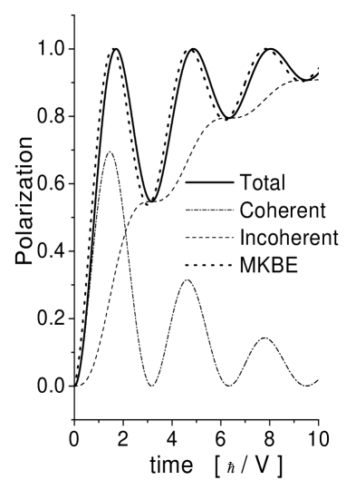
Figure 2: The ¹³C polarization (solid line) is composed by the sum of a coherent part (dash-dotted line) and an incoherent contribution (dashed line). For comparison, the evolution obtained with the secular approximation of Ref. [3] (dotted line) is shown denoted as MKBE. Parameters: $\Gamma/V=0.25$

Figure 2 shows the behavior of the ¹³C polarization. It can be seen that it reaches the value of 1 periodically, converging to the equilibrium value of 1 at the exponential rate $1/\tau_{2}$. The first maximum occurs at a relatively short time compared with $\tau_{2}.$ This feature is used in the spin swap operation by stopping rf irradiation (and hence the interaction) at a maximal transfer. The maxima in our curves of $P_{-1,0}(t)$ are always equal to one because of the symmetry adopted ($E_{0}=E_{-1}$). However, only the first maxima of the coherent component decaying as $\exp[-t/\tau_{2}],$ i.e. about 0.7 for our choice of parameters, would be useful in quantum information processing. The incoherent component of the polarization, having no definite phase relation with respect to the original state, bears no information on the quantum evolution. This can be observed by NMR interferometry as done in Refs. [18, 19]. In this case the observed polarization at ¹³C presents high frequency oscillations consequence of the interference between the polarization amplitude that survived at the ¹³C and the component returning after wandering in the ¹H system. This interference would be diminished if, in the last CP, one uses the second maximum.

Another interesting feature of Eqs. (12) and (13) is that they have zero slope for $t=0$ as can be seen in Fig 3. This expresses that the quantum nature of the problem has not disappeared within the present approximation, in contrast with the result obtained by using the secular approximation $\Gamma$ $\ll$ $V$, standard in NMR calculations [3]. Performing the same approximation as in Ref. [3], but considering $XY$ coupling between the system and the spin reservoir, we obtain for the normalized polarization of the ¹³C nucleus

$$P_{-1,0}(t)=1-\frac{\exp\{-\frac{t\Gamma}{\hbar}\}}{2}-\frac{\exp\{-\frac{t\Gamma}{\hbar}\}}{2}\cos(2Vt/\hbar).$$ (16)

Both Eqs. (13) and (16) are obtained considering the fast fluctuations approximation which leads to $\Gamma_{c}(\varepsilon)=$constant. However, comparing Eqs. (13) and (16) it can be seen that the main differences between them are the decrease of the swapping frequency and the extra phase that result from the Keldysh formalism. The frequency decrease is a natural effect of the damping in an harmonic oscillator and hence its meaning is clear. The extra phase provides the correct quadratic behavior for short times. Both effects would introduce corrections up to a 10% if one attempts an estimation of the dipolar frequency (here $2V/\hbar$) from the first experimental maximum. However, if the frequency is evaluated from the FT of the signal it differs from the dipolar one in a factor of $(1-(\frac{\Gamma}{2V})^{2})^{1/2}$. This can have important consequences when one attempts to perform a quantification of the ¹³C$-^{1}$H average distances [33].

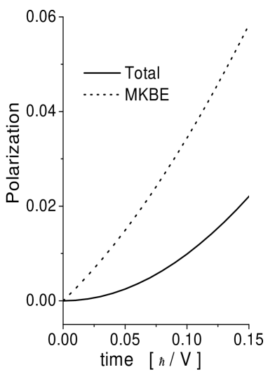
Figure 3: It is shown the short time regime for the Polarization function for the ${}^{13}C$ nucleous obtained within the Keldysh formalism (solid line) in contrast with the the evolution obtained with the seccular approximation (MKBE) of Ref. [3] (doted line). Parameters: $\Gamma/V=0.25$

4 Memory effects of the spin bath

The ¹³C polarization, $P_{-1,0}(t)$, in the Keldysh formalism arises from the coherent evolution of the initial particle density, for which the environment is a “sink”,  and an incoherent contribution where the bath acts as a particle “source”. This can be compared with the complementary framework. Instead of dealing with a “particle” problem let us consider it as a “hole” problem (Fig. 1 $(b)$ and $(c)$ respectively). On these grounds, at $t=0,$ all the sites are occupied except for the “hole” excitation at the $-1$-th site. See Fig. 1 $(c)$ where the black color stands for the hole excitation. At later times this excitation evolves in the system and also propagates through the reservoir. The “environment” does not have holes to inject back into the “system” but those evolved coherently from the initial hole (i.e. $\Sigma^{<}\equiv 0$). Here the environment is a perfect “sink”. Thus all the dynamics would be coherent, in the sense previously explained. If we add the result obtained in this case with that of Eq. (13) we obtain a one for all times consequence of the particle-hole symmetry. This is a particularly good test of the consistency of the formalism because in each result the “environment” is set in a different framework. It also shows that the background polarization does not contribute to the dynamics.

This “hole” picture can help us to get a very interesting insight on the dynamics in a case where the memory on the environment becomes relevant. Consider, for example, the case $V=V_{0}=V_{c}$ and $E_{0}=E_{-1}$. The finite version of this effective Hamiltonian applies to the actual experiments reported in Ref. [34]. In this case, the simplifying approximations of the fast fluctuations regime are not justified. However, the exact dynamics of the system can be analytically obtained if one considers an infinite chain. This enables the use of Eq. (10) to evaluate the propagator in the first term of Eq. (6). The integration gives the first Bessel function, hence:

$$P_{-1,0}(t)=1-\left|\frac{\hbar}{tV}J_{1}(2tV/\hbar)\right|^{2}.$$ (17)

A first observation is that the frequency above is roughly increased by a factor of two as compared with that in Eq. (15). Since the maxima of $P_{-1,0}$ are zeroth of the Bessel function it is clear that the frequency increases slightly with time. These are memory effects of the environment that are dependent on the interplay between the spectral density of the bath and that of the system.

We notice that the memory effect can also appear in other condition for the bath. For example, if the proton nuclei have random polarizations and the density excitation is at site $-1$, i.e. in Fig. 1 ($a$)  $\mathrm{f}_{n}(\varepsilon)=\left(\frac{1}{2}\right)$ for $n=0,1,..$ representing the ¹H sites filled up to the shaded region; and the ¹³C site with an occupation $\frac{1}{2}+\Delta P$. In this case the excitation propagates over a background level (shaded region) that does not contribute to the dynamics. The schematic view of this initial condition is equivalent to that of Fig. 1 ($c$) where now the black filling represents a particle excitation. The solution of the polarization is the first Bessel function, $P_{-1,-1}(t)=\left|\frac{\hbar}{tV}J_{1}(2tV/\hbar)\right|^{2}.$ Apart from the finite size mesoscopic effect, this is precisely the situation observed in Ref. [34], although without enough resolution for a quantitative comparison. The effect of a progressive modification of the swapping frequency is often observed in many experimental situations such as CP experiments. Depending on the particular system, the swapping frequency can accelerate or slow down. Reported examples are Fig. 5 on Ref. [19] and Fig. 4 on Ref. [35]. This simple example solved so far shows that environmental correlations have fundamental importance in the dynamics and deserve further attention.

5 Conclusions

Summarizing, we have solved the Schrödinger equation within the Keldysh formalism with a source boundary condition which results in an injection of quantum waves without definite phase relation with the initial state. The model proposed allowed us to consider the effect of the environment over the system via the decay of the initial state followed with an incoherent injection. We obtained analytical expressions for the polarization of each of the components of a ¹³C$-^{1}$H system coupled to a spin bath, improving the result obtained through the application of the secular approximation [3] in standard density matrix calculation.

Of particular interest is the inclusion of temporal correlations within the spin bath in a model which has exact solution. On one side, it enabled us to show a novel result: memory effects can produce a progressive change of the swapping frequency. On the other side, this results will serve to test approximate methods developed to deal with complex correlations.

In general, our analytical results based in the spin-particle mapping, allow a deeper understanding of the polarization dynamics. They may constitute a starting point for the study of other problems, such as different topologies [23] with XY interaction and the extension to dipolar and isotropic couplings.

Appendix A

Let us define the function

$$G_{0,0}^{\;<\,\mathrm{inc.}_{(N)}\,}(t_{2},t_{1})=\sum_{n,m}\int_{0}^{t_{2}}\int_{0}^{t_{1}}G_{0,m}^{R_{(N)}}(t_{2},t_{m})\Sigma_{m,n}^{\,\,<_{(N)}}(t_{m},t_{n})G_{n,0}^{A_{(N)}}(t_{n},t_{1})\mathrm{d}t_{m}\mathrm{d}t_{n},$$ (18)

which is the second term in Eq. (5). A similar expression holds for the coherent part. The manipulation that follows is independent on the subspace index ($N$), and we will keep it implicit. Rewriting the integrand in Eq.(18) as

$$G_{0,m}^{R}(t_{2},t_{m})\Sigma_{m,n}^{<}(t_{m},t_{n})G_{n,0}^{A}(t_{n},t_{1})$$

$$=G_{0,m}^{R\,\,}(t_{2}-t_{m},\tfrac{t_{2}+t_{m}}{2})\Sigma_{m,n}^{\;<\;}(t_{m}-t_{n},\tfrac{t_{m}+t_{n}}{2})G_{n,0}^{A\,}(t_{n}-t_{1},\tfrac{t_{n}+t_{1}}{2})$$

$$=\int\int\int G_{0,m}^{R\,\,}(\varepsilon_{R},\tfrac{t_{2}+t_{m}}{2})\Sigma_{m,n}^{\;<\;}(\varepsilon^{\prime},\tfrac{t_{m}+t_{n}}{2})G_{n,0}^{A\,}(\varepsilon_{A},\tfrac{t_{n}+t_{1}}{2})$$

$$\exp\left[-\mathrm{i}\varepsilon_{R}(t_{2}-t_{m})/\hbar\right]\exp\left[-\mathrm{i}\varepsilon^{\prime}(t_{m}-t_{n})/\hbar\right]\exp\left[-\mathrm{i}\varepsilon_{A}(t_{n}-t_{1})/\hbar\right]\tfrac{\mathrm{d}\varepsilon_{R}}{2\pi\hbar}\tfrac{\mathrm{d}\varepsilon^{\prime}}{2\pi\hbar}\tfrac{\mathrm{d}\varepsilon_{A}}{2\pi\hbar}.$$ (19)

Let’s define the macroscopic time as $t=\tfrac{1}{2}(t_{2}+t_{1})$ and the quantum correlation time $\delta t=t_{2}-t_{1}$ which have related time scales of the injection processes as $t_{i}=\frac{1}{2}\left(t_{m}+t_{n}\right)$ and $\delta t_{i}=t_{m}-t_{n}.$ These time scales are associated with  $\varepsilon=\frac{1}{2}\left(\varepsilon_{R}+\varepsilon_{A}\right),$ the energies characterizing the quantum correlation, and $\omega=\frac{1}{\hbar}\left(\varepsilon_{R}-\varepsilon_{A}\right)$ the frequencies in the observables. The argument in the exponential function becomes

$$\varepsilon_{R}t_{2}-\varepsilon_{R}t_{m}+\varepsilon_{A}t_{n}-\varepsilon_{A}t_{1}$$

$$=\varepsilon_{R}t+\varepsilon_{R}\tfrac{\delta t}{2}-\varepsilon_{R}t_{i}-\varepsilon_{R}\tfrac{\delta t_{i}}{2}+\varepsilon_{A}t_{i}-\varepsilon_{A}\tfrac{\delta t_{i}}{2}-\varepsilon_{A}t+\varepsilon_{A}\tfrac{\delta t}{2}$$

$$=\hbar\omega(t-t_{i})+\varepsilon\delta t-\varepsilon\delta t_{i},$$

and also

$$\varepsilon^{\prime}(t_{m}-t_{n})=\varepsilon^{\prime}\delta t_{i}.$$

The Green’s functions take the form

$$G_{0,m}^{R\,\,}(\varepsilon_{R},\tfrac{t_{2}+t_{m}}{2}) =G_{0,m}^{R\,\,}(\varepsilon+\tfrac{\hbar\omega}{2},\tfrac{t+t_{i}}{2}+\tfrac{\delta t+\delta t_{i}}{4})$$

$$G_{n,0}^{A\,}(\varepsilon_{A},\tfrac{t_{n}+t_{1}}{2}) =G_{n,0}^{A\,}(\varepsilon-\tfrac{\hbar\omega}{2},\tfrac{t+t_{i}}{2}-\tfrac{\delta t+\delta t_{i}}{4})$$

$$\Sigma_{m,n}^{\;<\;}(\varepsilon^{\prime},\tfrac{t_{m}+t_{n}}{2}) =\Sigma_{m,n}^{\;<\;}(\varepsilon^{\prime},t_{i}).$$

Finally due to the fact that the transformation have the property that its Jacobian is equal to one, we have $\mathrm{d}t_{m}\mathrm{d}t_{n}=\mathrm{d}t_{i}\mathrm{d}\delta t_{i}$ and $\mathrm{d}\varepsilon_{R}\mathrm{d}\varepsilon_{A}=\hbar\mathrm{d}\varepsilon\mathrm{d}\omega.$ Replacing all these expressions in the integral of Eq. (18) we have

$$\sum_{n,m}\int_{t_{0}}^{t_{2}}\int_{t_{0}}^{t_{1}}G_{0,m}^{R\,\,}(t_{2},t_{m})\Sigma_{m,n}^{\;<\;}(t_{m},t_{n})G_{n,0}^{A\,}(t_{n},t_{1})\mathrm{d}t_{m}\mathrm{d}t_{n}\\ =\int\int\int\int\int G_{0,m}^{R\,\,}(\varepsilon+\tfrac{\hbar\omega}{2},\tfrac{t+t_{i}}{2}+\tfrac{\delta t+\delta t_{i}}{4})\Sigma_{m,n}^{\;<\;}(\varepsilon^{\prime},t_{i})G_{n,0}^{A\,}(\varepsilon-\tfrac{\hbar\omega}{2},\tfrac{t+t_{i}}{2}-\tfrac{\delta t+\delta t_{i}}{4})\\ \times\exp\{-\mathrm{i}[\hbar\omega(t-t_{i})+\varepsilon\delta t-\varepsilon\delta t_{i}+\varepsilon^{\prime}\delta t_{i}]/\hbar\}\mathrm{d}t_{i}\mathrm{d}\delta t_{i}\frac{\mathrm{d}\varepsilon}{2\pi\hbar}\frac{\mathrm{d}\varepsilon^{\prime}}{2\pi\hbar}\frac{\mathrm{d}\omega}{2\pi}.$$

Then, we can express Eq. (18) as

$$G_{0,0}^{\;<\,\mathrm{inc.}}(t,\delta t)=\int G_{0,0}^{\;<\,\mathrm{inc.}}(\varepsilon,t)\exp\left[-\mathrm{i}\varepsilon\delta t/\hbar\right]\frac{\mathrm{d}\varepsilon}{2\pi\hbar},$$

and using the last two expressions we can identify

$$G_{0,0}^{\;<\,\mathrm{inc.}\,}(\varepsilon,t)=\\ \int\int\int\int G_{0,m}^{R\,\,}(\varepsilon+\tfrac{\hbar\omega}{2},\tfrac{t+t_{i}}{2}+\tfrac{\delta t+\delta t_{i}}{4})\Sigma_{m,n}^{\;<\;}(\varepsilon^{\prime},t_{i})G_{n,0}^{A\,}(\varepsilon-\tfrac{\hbar\omega}{2},\tfrac{t+t_{i}}{2}-\tfrac{\delta t+\delta t_{i}}{4})\\ \times\exp\left[-\mathrm{i}[\left(\hbar\omega(t-t_{i})-\varepsilon\delta t_{i}+\varepsilon^{\prime}\delta t_{i}\right)/\hbar\right]~{}\mathrm{d}t_{i}\mathrm{d}\delta t_{i}\frac{\mathrm{d}\omega}{2\pi}\frac{\mathrm{d}\varepsilon^{\prime}}{2\pi\hbar}.$$

A similar expression holds for the coherent term.

Integrating in energy we obtain $G_{0,0}^{\;<\,\,}(t,t).$ If we consider that the system Hamiltonian is time independent the last complex expression simplifies to

$$G_{0,0}^{\;<\,\mathrm{inc.}\,}(t,t)=\int_{t_{0}}^{t}\int_{-\infty}^{\infty}\int_{-\infty}^{\infty}\sum_{n,m}G_{0,m}^{R\,\,}(\varepsilon+\tfrac{\hbar\omega}{2})\Sigma_{m,n}^{\;<\;}(\varepsilon,t_{i})G_{n,0}^{A\,}(\varepsilon-\tfrac{\hbar\omega}{2})\\ \exp\left[-\mathrm{i}\omega(t-t_{i})\right]\frac{\mathrm{d}\omega}{2\pi}\frac{\mathrm{d}\varepsilon}{2\pi\hbar}\mathrm{d}t_{i},$$

which is similar to the second term in Eq. (6).

References

- [1] F. Meier, J. Levy, D. Loss, Phys. Rev. Lett. 90 (2003) 047901.
- [2] C.H. Bennet, D.P. DiVincenzo, Nature 404 (2000) 247.
- [3] L. Müller, A. Kumar, T. Baumann, R.R. Ernst, Phys. Rev. Lett. 32 (1974) 1402.
- [4] J.L. D’Amato, H.M. Pastawski, Phys. Rev. B 41 (1990) 7411.
- [5] J.P. Paz, W.H. Zurek, 72nd Les Houches Summer School on “Coherent Matter Waves”, July-August (1999).
- [6] W.H. Zurek, Rev. Mod. Phys. 75 (2003) 715.
- [7] L.A. Wu, D.A. Lidar, Phys. Rev. Lett. 88 (2002) 207902.
- [8] V.V. Dobrovitski, H.A. De Raedt, M.I. Katsnelson, B.N. Harmon, Phys. Rev. Lett. 90 (2003) 210401.
- [9] C.H. Tseng, S. Somaroo, Y. Sharf, E. Knill, R. Laflamme, T.F. Havel, D.G. Cory, Phys. Rev. A 62 (2000) 032309.
- [10] V. Mujica, M. Kemp, M.A. Ratner, J. Chem. Phys. 101 (1994) 6856.
- [11] S. Pleutin, H. Grabert, G.L. Ingold, A. Nitzan, J. Chem. Phys. 118 (2003) 3756.
- [12] Xin-Qi Li, Yi Jing Yan, Appl. Phys. Lett. 79 (2001) 2190.
- [13] N. Zimbovskaya, J. Chem. Phys. 118 (2003) 4.
- [14] A. Abragam, The principles of nuclear magnetism, Clarendon Press., Oxford (1961).
- [15] R.R. Ernst, G. Bodenhausen, A. Wokaun, Principles of nuclear magnetic resonance in one and two dimensions, Oxford University Press., Oxford (1987).
- [16] J.M. Taylor, A. Imamoglu, M.D. Lukin, Phys. Rev. Lett. 91 (2003) 246802.
- [17] H.M. Pastawski, P.R. Levstein, G. Usaj, Phys. Rev. Lett. 75 (1995) 4310.
- [18] H.M. Pastawski, G. Usaj, P.R. Levstein, Chem. Phys. Lett. 261 (1997) 329.
- [19] P.R. Levstein, G. Usaj, H.M. Pastawski, J. Chem. Phys. 108 (1998) 2718.
- [20] R.A. Jalabert, H.M. Pastawski, Phys. Rev. Lett. 86 (2001) 2490.
- [21] E.P. Danieli, H.M. Pastawski, P.R. Levstein, Chem. Phys. Lett. 384 (2004) 306.
- [22] H.M. Pastawski, G. Usaj, Phys. Rev. B 57 (1998) 5017.
- [23] E.P. Danieli, H.M. Pastawski, P.R. Levstein, Physica B 320 (2002) 351.
- [24] E.H. Lieb, T. Schultz, D.C. Mattis, Ann Phys. 16 (1961) 407.
- [25] C.D. Batista, G. Ortiz, Phys. Rev. Lett. 86 (2001) 1082.
- [26] L.V. Keldysh, ZhETF 47 (1964) 1515 [Sov. Phys.-JETP 20 (1965) 335].
- [27] G.D. Mahan, Many-Particle Physics, second edition, Plenum Press., New York, (1990).
- [28] P. Danielewicz, Ann. Phys. 152 (1984) 239.
- [29] H.M. Pastawski, Phys. Rev. B 46 (1992) 4053.
- [30] A. Pines, M.G. Gibby, J.S. Waugh, J. Chem. Phys. 56 (1972) 1776.
- [31] S.I. Doronin, E.B. Fel’dman, S. Lacelle, J. Chem. Phys. 117 (2002) 9646.
- [32] P.R. Levstein, H.M. Pastawski, J.L. D’Amato, J. Phys. Condens. Matter 2 (1990) 1781.
- [33] P. Bertani, J. Raya, P. Reinheimer, R. Gougeon, L. Delmotte, J. Hirschinger, Solid State Nucl. Magn. Reson. 13 (1999) 219.
- [34] Z.L. Mádi, B. Brutscher, T. Schulte-Herbrüggen, R. Brüschweiler, R.R. Ernst, Chem. Phys. Lett. 268 (1997) 300.
- [35] P.R. Levstein, A.K. Chattah, H.M. Pastawski, J. Raya, J. Hirschinger, J. Chem. Phys. 121 (2004) 7313.