Critical temperature for the two-dimensional attractive Hubbard Model

Abstract

The critical temperature for the attractive Hubbard model on a square lattice is determined from the analysis of two independent quantities, the helicity modulus, $\rho_{s}$, and the pairing correlation function, $P_{s}$. These quantities have been calculated through Quantum Monte Carlo simulations for lattices up to $18\times 18$, and for several densities, in the intermediate-coupling regime. Imposing the universal-jump condition for an accurately calculated $\rho_{s}$, together with thorough finite-size scaling analyses (in the spirit of the phenomenological renormalization group) of $P_{s}$, suggests that $T_{c}$ is considerably higher than hitherto assumed.

The attractive Hubbard modelMRR90 ; Wilson01 has been successfully used to elucidate a number of important and fundamental issues in both conventional and high-temperature (cuprate) superconductivity. The nature of the crossover between BCS superconductivity (at weak coupling, or small on-site attraction) and Bose-Einstein condensation of tightly bound pairs (strong coupling) has been shown to be smooth Leggett80 ; Randeria98 . The appearance of preformed pairs within a certain range of parameters in the normal phase, especially below a characteristic temperature, has been related to pseudogap behavior of high-temperature superconductors Randeria92 ; dS94 . Further, this model allows one to introduce disorder on the fermionic degrees of freedom Litak92 ; Scalettar99 and investigate the behavior near the quantum critical point of the two-dimensional insulator-superconductor transition; this provides an alternative to the dirty-boson picture Fisher90 to discuss the universal conductivity Hsu95 . The attractive Hubbard model with a periodic modulation of $U$ has been used to interpret superconductivity in layered structures Paiva .

A basic concern has run through many of these calculations, in particular those based on Quantum Monte Carlo (QMC) simulations. In two dimensions, there is a consensus that the early QMC phase diagram Scalettar89 ; Moreo91 – in the space of critical temperature, $T_{c}$, electronic density, $\langle n\rangle$, and magnitude of the on-site attraction, $|U|$ – is qualitatively correct. However, some serious quantitative discrepancies have emerged over the years, pointing towards higher critical temperatures; see, e.g., the Bogoliubov-Hartree-Fock (BHF) approach of Ref. Denteneer91-93, . Our purpose here is to examine the dependence of $T_{c}$ with $\langle n\rangle$, for fixed $U$, by resorting to a much wider (namely, larger system sizes and several electronic densities) set of QMC data, together with alternative procedures to locate the critical temperature. Establishing an accurate value for this most fundamental property of the model is important, especially as the physics of variants of the attractive Hubbard Hamiltonian is explored, and comparisons are made to the original system.

The model is defined by the Hamiltonian

$${\cal H}= -t\sum_{\langle{\bf i},{\bf j}\rangle,\,\sigma}\left(c_{{\bf i}\sigma}^{\dagger}c_{{\bf j}\sigma}^{\phantom{\dagger}}+{\rm H.c.}\right)-\mu\sum_{\bf i}\left(n_{{\bf i}\uparrow}^{\phantom{\dagger}}+n_{{\bf i}\downarrow}^{\phantom{\dagger}}\right)$$ (1)

$$-|U|\sum_{\bf i}\left(n_{{\bf i}\uparrow}^{\phantom{\dagger}}-\frac{1}{2}\right)\left(n_{{\bf i}\downarrow}^{\phantom{\dagger}}-\frac{1}{2}\right)$$

where $c_{{\bf i}\sigma}^{\phantom{{}^{\dagger}}}$ ($c_{{\bf i}\sigma}^{{}^{\dagger}}$) destroys (creates) an electron with spin $\sigma$ on site ${\bf i}$ of a square lattice, $\langle{\bf i},{\bf j}\rangle$ denotes nearest neighbor sites, $n_{{\bf i}\sigma}\equiv c_{{\bf i}\sigma}^{{}^{\dagger}}c_{{\bf i}\sigma}^{\phantom{{}^{\dagger}}}$, $|U|$ is the strength of the attractive interaction and $\mu$ is the chemical potential. From now on, all energies are expressed in units of the hopping amplitude, $t$, and we also set $k_{B}=1$.

At half filling (which corresponds to the particle-hole symmetric point, $\mu=0$), the degeneracy of charge-density wave (CDW) and singlet superconducting (SS) correlations leads to a three-component order parameter shiba ; the transition temperature is therefore suppressed to zero. Away from half-filling, CDW correlations are suppressed and a finite temperature Kosterlitz-Thouless (KT) transition kt into a SS phase takes place Moreo91 ; Assaad94 ; this phase has only algebraically decaying correlations for $0<T\leq T_{c}$. Further, close to half filling an exact mapping onto the two-dimensional Heisenberg antiferromagnetic model in a magnetic field leads to Scalettar89 ; Moreo91 $T_{c}\simeq-2\pi J/\ln|1-\langle n\rangle|$, so that $T_{c}$ rises sharply from zero as one dopes away from $\langle n\rangle=1$.

We start by employing the analysis of Ref. Moreo91, to new data for the SS pairing correlation function,

$$P_{s}=\langle\Delta^{\dagger}\Delta+\Delta\Delta^{\dagger}\rangle,$$ (2)

with

$$\Delta^{\dagger}=\frac{1}{\sqrt{N}}\sum_{i}c_{{\bf i}\uparrow}^{{}^{\dagger}}c_{{\bf i}\downarrow}^{{}^{\dagger}}.$$ (3)

For $0<T\leq T_{c}$, one expects

$$\Gamma(r)\equiv\langle c_{{\bf i}\uparrow}^{\dagger}c_{{\bf i}\downarrow}^{\dagger}c_{{\bf j}\downarrow}^{\phantom{\dagger}}c_{{\bf j}\uparrow}^{\phantom{\dagger}}+{\rm H.c.}\rangle\sim r^{-\eta(T)}$$ (4)

where $r\equiv|{\bf i}-{\bf j}|$, and $\eta(T)$ increases monotonically between $\eta(0)=0$ and $\eta(T_{c})=1/4$ kt ; Berche02 .

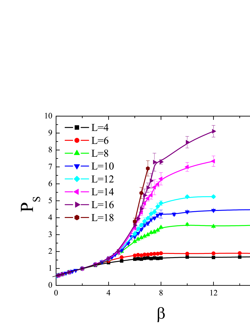
Figure 1: (Color online) $P_{s}$ as a function of $\beta\equiv 1/T$ for $\langle n\rangle=0.5$ and different lattice sizes, $L$.

The finite-size scaling behavior of $P_{s}$ is therefore obtained upon integration of $\Gamma(r)$ over a two-dimensional system of linear dimension $L$. One then has Moreo91

$$P_{s}=L^{2-\eta(T_{c})}f(L/\xi),\ \ \ L\gg 1,\ T\to T_{c}^{+},$$ (5)

with

$$\xi\sim\exp\left[\frac{A}{(T-T_{c})^{1/2}}\right];$$ (6)

in the thermodynamic limit, one recovers $P_{s}\sim\xi^{7/4}$. For completeness, one should mention that since $\eta\to 0$ as $T\to 0$, the system displays long-range order in the ground state, so that a ‘spin-wave scaling’ is expected to hold Huse88 :

$$\frac{P_{s}}{L^{2}}=|\Delta_{0}|^{2}+\frac{C}{L},$$ (7)

where $\Delta_{0}$ is the superconducting gap function at zero temperature, and $C$ is a $|U|$-dependent constant.

Similarly to Ref. Moreo91, , here we use the determinant QMC algorithm qmc to calculate $P_{s}$. Typically our data have been obtained after 500 warming-up steps followed by 50,000 sweeps through the lattice. The discretized imaginary-time interval qmc was set to $\Delta\tau=0.125$, which is small enough for the results not to depend on this choice in any significant way.

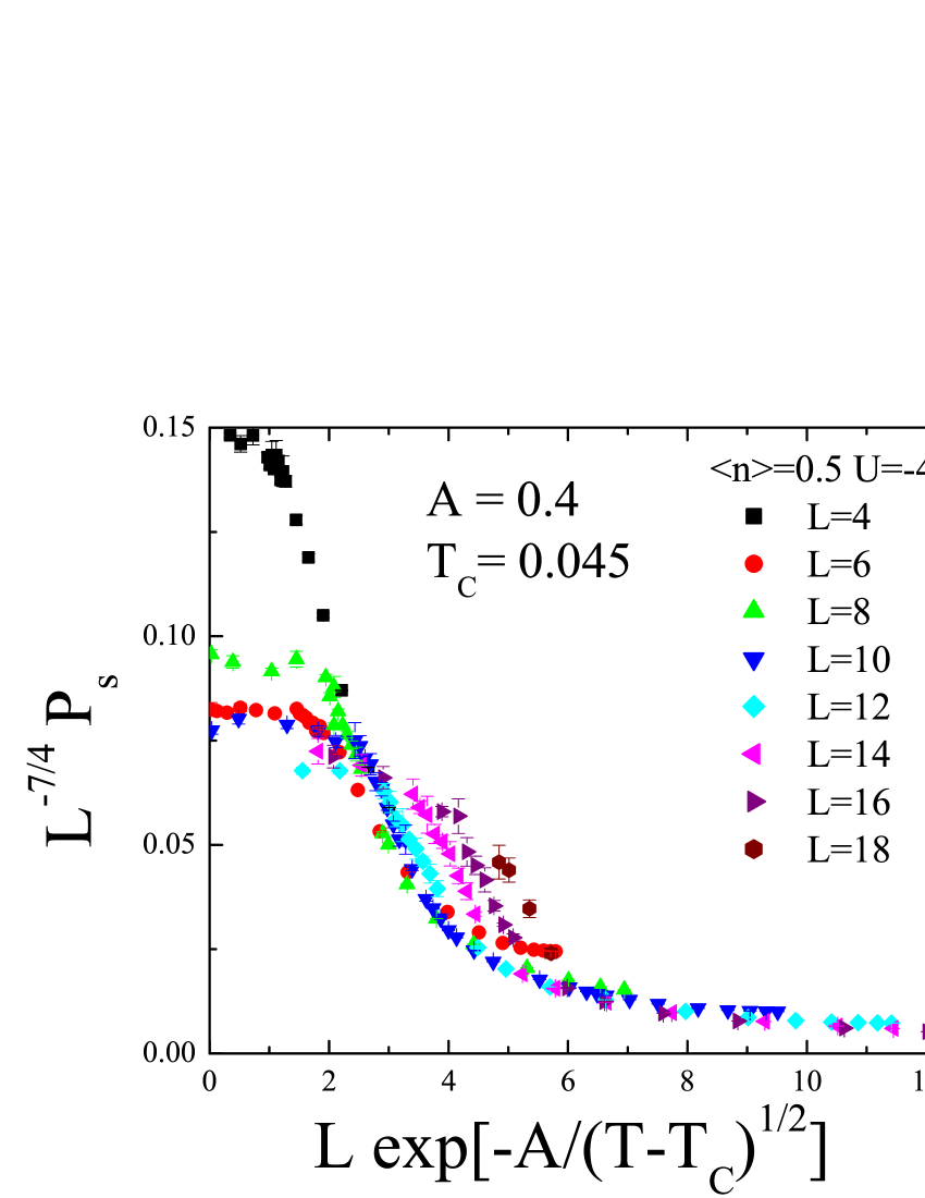
Figure 2: (Color online) Rescaled $P_{s}$ as a function of $w\equiv L\exp[-A/(T-T_{c})^{1/2}]$ for $\langle n\rangle=0.5$ and different lattice sizes, $L$. The values for $A$ and $T_{c}$ are the ones determined in Ref. Moreo91, .

In Fig. 1 we show raw data for $P_{s}$ as a function of $(1/T)$, for fixed density, $\langle n\rangle=0.5$ and $U=-4$, and for different lattice sizes. The crossover between temperature- and size-limited regimes is described by finite-size scaling (FSS) theory Cardy and appears as a levelling off of $P_{s}$ below a certain temperature for each system size. Before a more quantitative scaling analysis, we can already see a suggestion that $T_{c}$ is around 1/6 from the raw $P_{s}$ data. In general, at temperatures for which correlations are short ranged, a structure factor like $P_{s}$ is independent of lattice size. As $T$ is decreased, the point at which the structure factor begins growing with lattice size signals the temperature at which the correlation length $\xi$ is becoming large (comparable to the lattice size $L$), thus providing a crude estimate of $T_{c}$. The subsequent plateau at low temperatures occurs when $\xi>>L$. This crossover is contemplated by the FSS form, Eq. (5), which can be invoked to determine $T_{c}$ by plotting $L^{-7/4}P_{s}$ as a function of of $w\equiv L\exp[-A/(T-T_{c})^{1/2}]$, at a given $U$, for different system sizes, with $T_{c}$ and $A$ being adjusted to give the best possible data collapse, as done in Ref. Moreo91, . Figure 2 shows the resulting scaling plot, in which the values $A=0.4$ and $T_{c}=0.045$ were determined in Ref. Moreo91, . With our substantially increased amount of data points it becomes clear that the data collapse onto a single curve with the parameters $A$ and $T_{c}$ of Ref. Moreo91, becomes rather unsatisfactory. We furthermore note that Eq. (6) is expected to hold only for $t\lesssim 10^{-2}$ ($t\equiv(T-T_{c})/T_{c}$), see, e.g., Ref. gupta, . For the value of $T_{c}$ used in Fig. 2, only few data obtained for $L=4,6,8,10$ in Ref. Moreo91, satisfy this criterion.

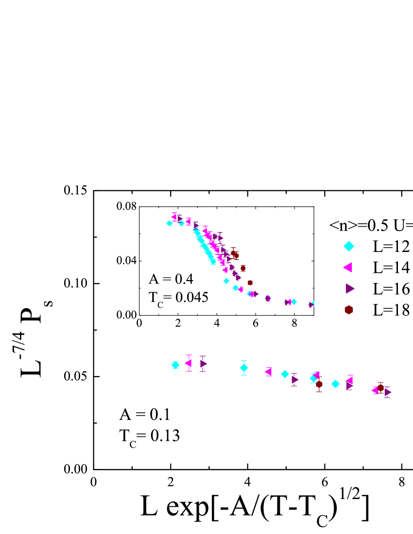
Figure 3: (Color online) Same as Fig. 2, but with $A$ and $T_{c}$ determined from the present data. Inset shows same system sizes, with $A$ and $T_{c}$ from Ref. Moreo91, .

We therefore obtain new values of $A$ and $T_{c}$ from our expanded data set. We disregard the data from the smallest system sizes, $L=4$ (which, additionally, has a special topology, being equivalent to a $2\times 2\times 2\times 2$ four-dimensional lattice), $L=6$, $L=8$ and also $L=10$; as we will see below, the SS pairing correlation function presents large finite size effects for these lattice sizes. Furthermore, we only include data points for temperatures $T$ for which Eq. (6) is expected to hold (see above). Fig. 3 clearly shows that, for the larger latices, our newly determined parameters $A=0.1$ and critical temperature $T_{c}=0.13$ render a much better data collapse than the old parameters.

The present analysis shows that the estimates of $T_{c}$ obtained in Ref. Moreo91, can be quantitatively quite unreliable. In our opinion, this is due to the fact that the finite-size behaviour of $P_{s}$, Eqs. (5)-(6), follows from an analysis which is valid only for large enough lattice sizes, since it involves the binding-unbinding of rather large structures (vortices) in the KT transition kt . Moreover, the parameters $A$ and $T_{c}$ that have to be found via data fitting both reside in an exponent, resulting in large uncertainties for the individual fitted parameters. Although the lattice sizes used in the present study may not be large enough to determine $T_{c}$ with high accuracy, our result is bound to be an improvement and in any case indicates that the actual $T_{c}$ may be much larger (by even a factor of 3) than believed sofar.

This tendency towards higher critical temperatures appears as well in a completely independent analysis, based on the behavior of the helicity modulus (HM). The latter is a measure of the response of the system in the ordered phase to a ‘twist’ of the order parameter Fisher73 , and can be expressed in terms of the current-current correlation functions as follows Scalapino92

$$\rho_{s}=\frac{D_{s}}{4\pi e^{2}}=\frac{1}{4}[\Lambda^{L}-\Lambda^{T}],$$ (8)

where $D_{s}$ is the superfluid weight, and

$$\Lambda^{L}\equiv\lim_{q_{x}\to 0}\Lambda_{xx}(q_{x},q_{y}=0,\omega_{n}=0),$$ (9)

and

$$\Lambda^{T}\equiv\lim_{q_{y}\to 0}\Lambda_{xx}(q_{x}=0,q_{y},\omega_{n}=0),$$ (10)

are, respectively, the limiting longitudinal and transverse responses, with

$$\Lambda_{xx}(\vec{q},\omega_{n})=\sum_{\vec{\ell}}\int_{0}^{\beta}d\tau\ e^{i\vec{q}\cdot\vec{\ell}}e^{i\omega_{n}\tau}\Lambda_{xx}(\vec{\ell},\tau),$$ (11)

where $\omega_{n}=2n\pi T$;

$$\Lambda_{xx}(\vec{\ell},\tau)=\langle j_{x}(\vec{\ell},\tau)j_{x}(0,0)\rangle,$$ (12)

where

$$j_{x}(\vec{\ell},\tau)=e^{{\cal H}\tau}[it\sum_{\sigma}(c_{\vec{\ell}+\hat{x},\sigma}^{{}^{\dagger}}c_{\vec{\ell},\sigma}-c_{\vec{\ell},\sigma}^{{}^{\dagger}}c_{\vec{\ell}+\hat{x},\sigma}]e^{-{\cal H}\tau}$$ (13)

is the $x$-component of the current density operator; see Ref. Scalapino92, for details.

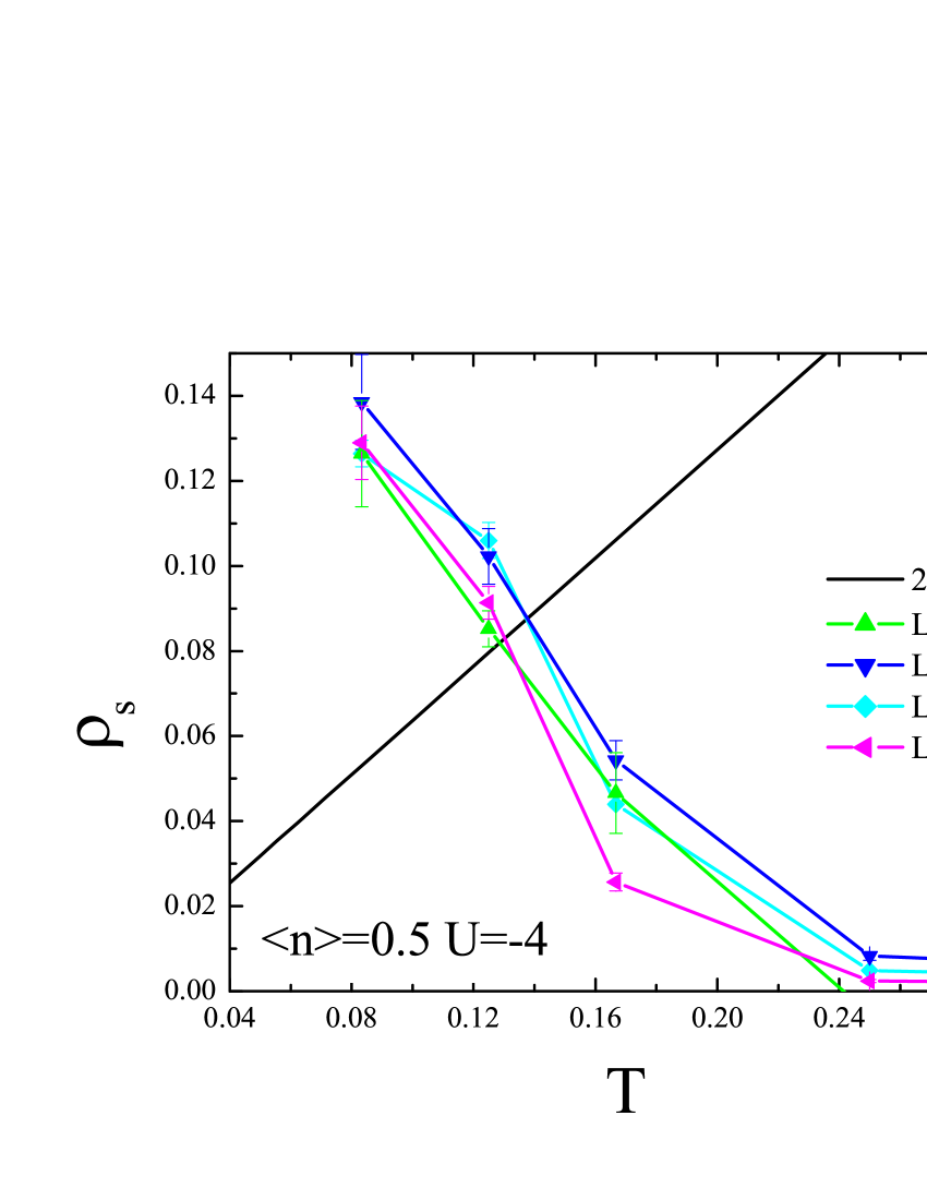
Figure 4: (Color online) Helicity modulus as a function of temperature for $\langle n\rangle=0.5$ and different lattice sizes, $L$. The straight line corresponds to $2T/\pi$.

At the KT transition, the following universal-jump relation involving the helicity modulus holds Nelson77 :

$$T_{c}=\frac{\pi}{2}\rho_{s}^{-},$$ (14)

where $\rho_{s}^{-}$ is the value of the helicity modulus just below the critical temperature. Thus we can obtain $T_{c}$ by plotting $\rho_{s}(T)$, and looking for the intercept with $2T/\pi$. This procedure has been used before, with $\rho_{s}$ calculated within a Bogoliubov-Hartree-Fock (BHF) approximation Denteneer91-93 ; Denteneer94 ; since transverse current-current correlations were neglected, $\rho_{s}$ is likely to have been overestimated, and the ensuing $T_{c}$’s may have been too high. Here we calculate both $\Lambda^{L}$ and $\Lambda^{T}$ by QMC simulations to obtain $\rho_{s}$ through Eq. (8); a typical example of $\rho_{s}(T)$, for $\langle n\rangle=0.5$, is shown in Fig. 4. We see that finite-size effects are not too drastic, since all curves cross the straight line within a small range of temperatures; that is, from Fig. 4 we can estimate $T_{c}=0.14\pm 0.02$.

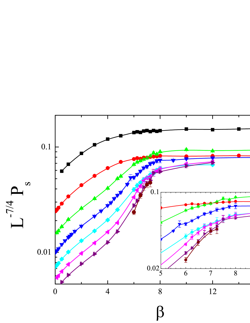
Figure 5: (Color online) Logarithm-linear plot for the rescaled $P_{s}$ as a function of $\beta$, for $\langle n\rangle=0.5$ and for different lattice sizes, $L$, symbols are the same as in Fig. 2. The inset shows a blow-up of the region centered about $\beta=7$. No parameters are adjusted.

In order to check the robustness of this method, we can extract $T_{c}$ from $P_{s}$ through a ‘phenomenological renormalization group’ (PRG) Nightingale82 ; dS81 analysis, provided some subtleties peculiar to the KT transition are kept in mind. Since $\xi\to\infty$ for all $T<T_{c}$, Eq. (5) implies that curves for $L^{-7/4}P_{s}(L,\beta)$, when plotted as functions of $\beta$, and for different $L$, should all merge for $\beta>\beta_{c}$. Figure 5 shows that this characteristic feature only sets in for the largest system sizes, namely, $L\geq 12$, from which we can infer $\beta_{c}=7.5\pm 0.25$; these error bars are somewhat arbitrary, and result from visual inspection. It should be stressed that this estimate for $\beta_{c}$ agrees remarkably well with the one obtained from the helicity modulus, indicating the robustness of both procedures to extract $T_{c}$. Interestingly, we should notice that the curves for $L=6$ and 8 cross each other (as in an ordinary second order transition) at $\beta\simeq 7$, which is very close to $\beta_{c}$ estimated from the larger systems. Therefore, within the context of PRG, for the smallest sizes a KT transition appears as an ordinary transition, only crossing over to the merging feature for the largest sizes.

The critical temperature has been estimated for other electronic densities, $\langle n\rangle=0.1$ (HM and PRG), 0.3 (PRG), 0.7 (PRG), and 0.875 (HM and PRG); all PRG plots display the crossing and merging tendency observed for $\langle n\rangle=0.5$. The resulting phase diagram is shown in Fig. 6; for comparison, we also plot the early QMC results Moreo91 , the parquet data from Luo and Bickers Luo93 , and the estimates from the BHF approximation Denteneer91-93 . While close to half filling all results (but BHF) are in fair agreement, for larger dopings agreement is only found between the results from PRG and those from the helicity modulus. The inescapable conclusion is that the critical temperature for the superconducting transition in the attractive Hubbard model is actually higher than previously assumed.

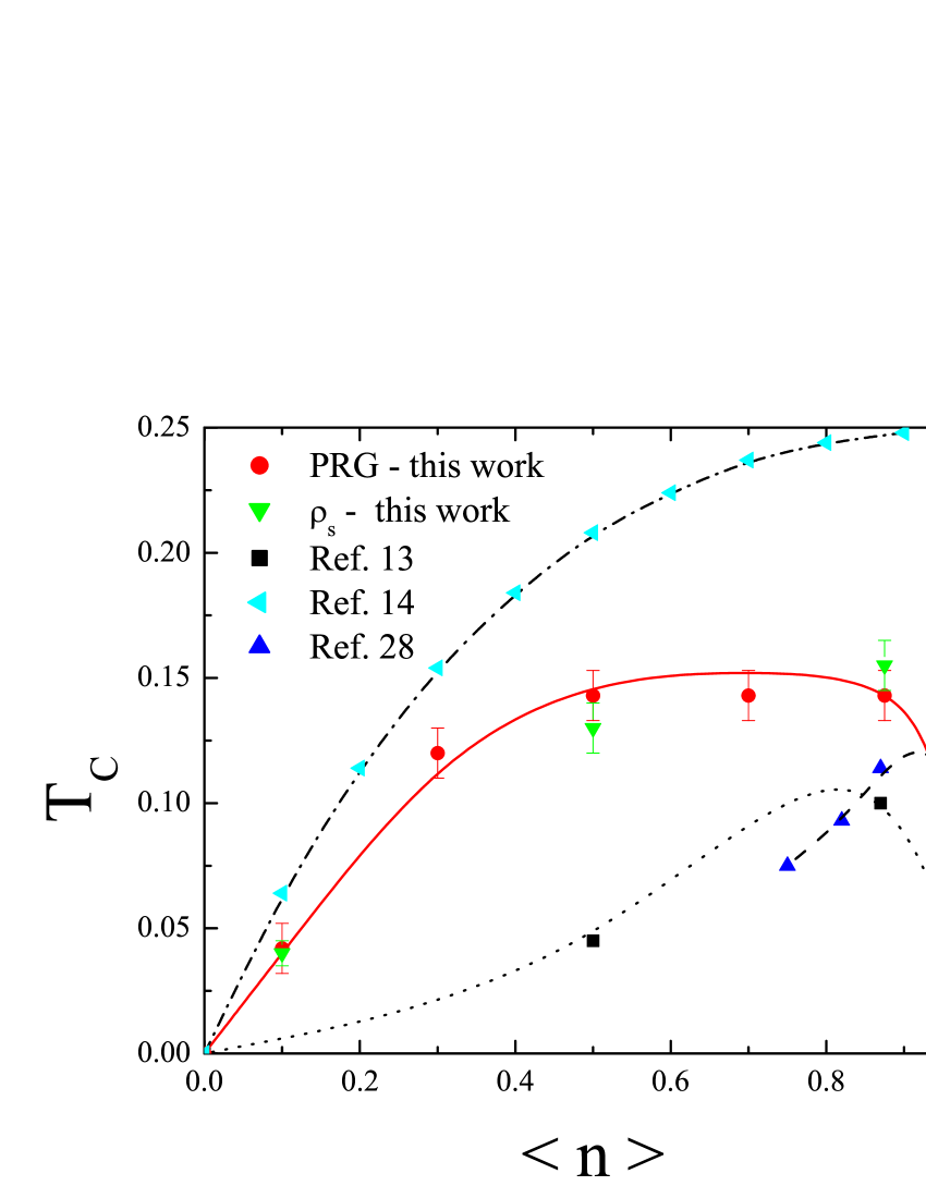
Figure 6: (Color online) Critical temperature as a function of band-filling, obtained by different methods. All lines through data points are guides to the eye.

In summary, we have established very reliable estimates for the critical temperature of the square-lattice attractive Hubbard model. This is done by finding quantitative agreement between entirely different procedures to extract $T_{c}$ from two independent correlation functions (both computed by determinant QMC). As a result, the critical temperature is found to be substantially higher than the currently accepted values, also obtained using QMC, but with a different data analysis; as expected, they are also substantially lower than estimates obtained within a Hartree-Fock/mean field approximation.

- (1) R. Micnas, J. Ranninger, and S. Robaszkiewicz, Rev. Mod. Phys. 62, 113 (1990).
- (2) J.A. Wilson, J.Phys.: Condens. Matter 13, R945 (2001).
- (3) A.J. Leggett, in Modern Trends in the Theory of Condensed Matter, edited by A. Pekalski and J. Przystawa (Springer, Berlin, 1980).
- (4) M. Randeria, in Proceedings of the International School of Physics ”Enrico Fermi”, edited by G. Iadonisi, J.R. Schrieffer, and M. Chiofalo (IOS Press, Amsterdam, 1998).
- (5) M. Randeria, N. Trivedi, A. Moreo, and R.T. Scalettar, Phys. Rev. Lett. 69, 2001 (1992).
- (6) R.R. dos Santos, Phys. Rev. B50, 635 (1994).
- (7) G. Litak, K.I. Wysokiski, R. Micnas and S. Robaszkiewicz, Physica C 199, 191 (1992).
- (8) R.T. Scalettar, N. Trivedi, and C. Huscroft, Phys. Rev. B59, 4364 (1999).
- (9) M. P. A. Fisher, G. Grinstein, and S. M. Girvin, Phys. Rev. Lett. 64, 587 (1990).
- (10) S.-Y. Hsu, J. A. Chervenak, and J. M. Valles, Jr, Phys. Rev. Lett. 75, 132 (1995).
- (11) T. Paiva, M. El Massalami, and R.R. dos Santos, J. Phys: Condens. Matter 15, 7917 (2003).
- (12) R.T. Scalettar, E.Y. Loh, Jr., J.E. Gubernatis, A. Moreo, S.R. White, D.J. Scalapino, R.L. Sugar, and E. Dagotto, Phys. Rev. Lett. 62, 1407 (1989).
- (13) A. Moreo and D.J. Scalapino, Phys. Rev. Lett. 66, 946 (1991).
- (14) P.J.H. Denteneer, G. An and J.M.J. van Leeuwen, Europhys. Lett. 16, 5 (1991); Phys. Rev. B47, 6256 (1993).
- (15) H. Shiba, Progr. Theor. Phys. 48, 2171 (1972).
- (16) J.M. Kosterlitz and D.J. Thouless, J.Phys. C 6, 1181 (1973).
- (17) F. F. Assaad, W. Hanke, and D. J. Scalapino, Phys. Rev. B49, 4327 (1994).
- (18) B. Berche, A. Farinas Sanchez, and R. Paredes, Europhys. Lett. 60, 539 (2002).
- (19) D.A. Huse, Phys. Rev. B37, 2380 (1988).
- (20) R. Blankenbecler, R. L. Sugar, and D. J. Scalapino, Phys. Rev. D24, 2278 (1981); S. R. White, D. J. Scalapino, R. L. Sugar, E. Y. Loh, Jr., J. E. Gubernatis, and R. T. Scalettar, Phys. Rev. B40, 506 (1989); R. R. dos Santos, Braz. J. Phys. 33, 36 (2003).
- (21) J.L. Cardy, Finite-size scaling in “Current Physics - Sources and Comments”, Vol. 2 (North-Holland, Amsterdam, 1988).
- (22) R. Gupta and C.F. Baillie, Phys. Rev. B45, 2883 (1992).
- (23) M. E. Fisher, M. N. Barber, and D. Jasnow, Phys. Rev. A8, 1111 (1973).
- (24) D. J. Scalapino, S. R. White, and S. C. Zhang, Phys. Rev. Lett. 68, 2830 (1992); Phys. Rev. B47, 7995 (1993).
- (25) D. R. Nelson and J.M. Kosterlitz, Phys. Rev. Lett. 39, 1201 (1977).
- (26) P. J. H. Denteneer, Phys. Rev. B49, 6364 (1994).
- (27) M.P. Nightingale, J. Appl. Phys. 53, 7927 (1982).
- (28) R.R. dos Santos and L. Sneddon, Phys. Rev. B23, 3541 (1981).
- (29) J. Luo and N.E. Bickers, Phys. Rev. B48, 15983 (1993).