Phase equilibria and fractionation in a polydisperse fluid

Abstract

We describe how Monte Carlo simulation within the grand canonical ensemble can be applied to the study of phase behaviour in polydisperse fluids. Attention is focused on the case of fixed polydispersity in which the form of the ‘parent’ density distribution $\rho^{\circ}(\sigma)$ of the polydisperse attribute $\sigma$ is prescribed. Recently proposed computational methods facilitate determination of the chemical potential distribution conjugate to $\rho^{\circ}(\sigma)$. By additionally incorporating extended sampling techniques within this approach, the compositions of coexisting (‘daughter’) phases can be obtained and fractionation effects quantified. As a case study, we investigate the liquid-vapor phase equilibria of a size-disperse Lennard-Jones fluid exhibiting a large ($\delta=40\%$) degree of polydispersity. Cloud and shadow curves are obtained, the latter of which exhibit a high degree of fractionation with respect to the parent. Additionally, we observe considerable broadening of the coexistence region relative to the monodisperse limit.

I Introduction

Many complex fluids, whether natural or synthetic in origin, comprise mixtures of similar rather than identical constituents. Examples are to be found in a host of soft matter materials. For instance, a colloidal dispersion may contain particles which exhibit a range of sizes, surface charge or chemical character; while many synthetic materials contain macromolecules having a range of chain lengths. This dependence of particle properties on one or more continuous parameters is termed polydispersity. It affects the performance of materials in applications ranging from foodstuffs to polymer processing LARSON99 .

In describing polydisperse systems, it is usual to label the polydisperse attribute by a continuous variable $\sigma$. The state of the system is then specified by a density distribution $\rho(\sigma)$ measuring the number density of particles of each $\sigma$. Certain systems such as micelles, may exhibit variable polydispersity in which the form of $\rho(\sigma)$ depends on the prevailing chemical and thermodynamic conditions. Others such as colloids and polymers exhibit so-called fixed polydispersity because $\rho(\sigma)$ is set by the synthesis of the fluid. In this letter we shall focus on the latter case.

Polydisperse fluids differ from their monodisperse counterparts in a variety of aspects. Principal among these is the much richer character of their phase behaviour SOLLICH02 . This richness is traceable to fractionation effects. At phase coexistence, particles of each $\sigma$ may partition themselves unevenly between two (or more) coexisting ‘daughter’ phases as long as–due to particle conservation–the overall composition $\rho^{\circ}(\sigma)$ of the ‘parent’ phase is maintained. This partitioning alters the character of phase diagrams. For example, the conventional liquid-gas binodal of a monodisperse system (which connects the ends of tie-lines in a density-temperature diagram) splits into a ‘cloud’ and a ‘shadow’ curve. These give, respectively, the density at which phase coexistence first occurs and the density of the incipient phase; the curves do not coincide because the shadow phase in general differs in composition from the parent. Only recently has experimental work started to elucidate in a systematic fashion the generic consequences of fractionation for phase coexistence properties EVANS98 ; FAIRHURST04 ; HEUKELUM03 .

Computational solutions for dealing with polydispersity have generally focused on the semi-grand canonical ensemble (SGCE). Within this framework, the instantaneous form of $\rho(\sigma)$ is permitted to fluctuate under the control of a distribution of chemical potential differences $\mu_{d}(\sigma)$, subject to a fixed overall number of particles. Use of such an approach is attractive because it permits the sampling of many different realizations of the ensemble of particle sizes, thereby ameliorating finite-size effects. For the investigation of phase coexistence, the SGCE has been combined with Gibbs-Duhem integration BOLHUIS ; KOFKE93 and Gibbs ensemble simulations STAPLETON ; KRISTOF . However, these studies were restricted to the case of variable polydispersity; no attempts were made to target a specific form of $\rho(\sigma)$ or determine cloud and shadow curves.

The computational difficulties associated with tackling fixed polydispersity are potentially quite severe: one needs to determine that form of the chemical potential distribution $\mu(\sigma)$ for which the ensemble averaged composition distribution $\bar{\rho}(\sigma)$ matches the target i.e. the prescribed parent $\rho^{\circ}(\sigma)$. Unfortunately, the chemical potential distribution is unavailable a priori, it being an unknown functional (i.e. $\mu(\sigma)=\mu[\rho^{\circ}(\sigma)]$), of the parent. Recently however, techniques have been developed that efficiently overcome this difficulty within the framework of a full grand canonical ensemble (GCE) WILDING02 ; ESCOBEDO01 ; WILDING03 . The latter is particular well suited to the study of fluid phase transitions due to the fluctuating overall particle number. In this letter we demonstrate that when combined with extended sampling methods, the new techniques facilitate the detailed and efficient study of phase behaviour in fluids of fixed polydispersity.

II Computational aspects

The grand canonical ensemble Monte Carlo algorithm we employ has been described in ref. WILDING02 and invokes four types of operation: particle displacements, deletions, insertions, and resizing. The polydisperse attribute $\sigma$ is itself represented as a strictly continuous variable, subject to some upper bound $\sigma_{c}$. However, observables such as the instantaneous composition distribution $\rho(\sigma)$ are accumulated in the form of a histogram by discretising the $\sigma$ domain into a prescribed number of bins. This discretisation also applies to the chemical potential distribution $\mu(\sigma)$, i.e. all particles whose $\sigma$ values is encompassed by the same bin are subject to an identical chemical potential.

The form of the ensemble averaged composition distribution $\bar{\rho}(\sigma)$ is controlled by $\mu(\sigma)$, via its role in the acceptance probabilities for particle transfers and resizing moves. For fixed polydispersity one wishes to match $\bar{\rho}(\sigma)$ to the desired parent distribution. The latter can be written as

$$\rho^{\circ}(\sigma)=n_{0}f(\sigma),$$ (1)

where $n_{0}=N/V$ is the overall particle number density, while $f(\sigma)$ is a prescribed normalized shape function. Since $\rho^{\circ}(\sigma)$ may vary only in terms of its scale $n_{0}$, the system is constrained to traverse a dilution line in the full phase space of possible compositions. The task is then to determine, as a function of temperature, the form of $\mu(\sigma)$ along the dilution line. More specifically, we seek the intersection of the dilution line with a coexistence region. Recently developed simulation techniques facilitate this, as we now summarize.

The non-equilibrium potential refinement (NEPR) scheme WILDING03 permits the efficient iterative determination of $\mu[\rho^{\circ}(\sigma),T]$, from a single simulation run, and without the need for an initial guess of its form. To achieve this, the method continually updates $\mu(\sigma)$ in such as way as to minimize the deviation of the instantaneous density distribution $\rho(\sigma)$ from the target form (i.e. the parent). However, tuning $\mu(\sigma)$ in this manner clearly violates detailed balance. To counter this, successive iterations reduce the degree of modification applied to $\mu(\sigma)$, thereby driving the system towards equilibrium and ultimately yielding the equilibrium form of $\mu[\rho^{\circ}(\sigma),T]$.

For the purpose of exploring phase diagrams, Histogram Extrapolation (HE) techniques have proved invaluable HR . In the present context, their use permits histogram of observables accumulated at one $\mu(\sigma)$ to be reweighted to estimate observables at some other $\mu(\sigma)$. In ref. WILDING02 we have shown how HE can be combined with a minimization scheme, to track a dilution line in a stepwise fashion. We shall deploy this approach again in the present study.

Simulation studies of phase coexistence present distinctive challenges. Principal among these is the large free energy (surface tension) barrier separating the coexisting phases. In order to accurately locate coexistence points, a sampling scheme must be utilized which enables this barrier to be surmounted BRUCE03 . One such scheme is multicanonical preweighting, which utilizes a weight function in the MC acceptance probabilities, in order to encourage the simulation to sample the interfacial configurations of low probability BERG92 . At a given coexistence state point, the requisite weight function takes the form of an approximation to the inverse of the distribution of the fluctuating number density, $p(n)$, with $n=N/V$. While specialized techniques allow determination of $p(n)$ from scratch, in situations where one wishes to track a fluid-fluid phase boundary, prior determination of a weight function is unnecessary provided one commences from the vicinity of the critical point where the barrier to inter-phase crossings is small. Data accumulated here can be used (together with HE) to provide estimates of suitable multicanonical weight functions at lower temperatures WILDING95 where the barrier height is greater.

III Model

The techniques outlined above have been deployed to obtain the liquid-vapor coexistence properties of a fluid of particles interacting via a pairwise potential of the Lennard-Jones (LJ) form:

$$U(r_{ij},\sigma_{ij})=4\epsilon\left[\left(\frac{\sigma_{ij}}{r_{ij}}\right)^{12}-\left(\frac{\sigma_{ij}}{r_{ij}}\right)^{6}\right]\>,$$ (2)

with $\sigma_{ij}=(\sigma_{i}+\sigma_{j})/2$. A cutoff was applied to this potential for particle separations $r_{ij}>2.5\sigma_{ij}$.

The polydispersity enters solely through the distribution of diameters $\sigma_{i}$. Our algorithm finds that $\mu(\sigma)$ for which the diameters are distributed according to $f(\sigma)$ given a choice for $n_{0}$ (cf. eq. 1). We have assigned $f(\sigma)$ the Schulz form:

$$f(\sigma)=\frac{1}{z!}\left(\frac{z+1}{\bar{\sigma}}\right)^{z+1}\sigma^{z}\exp\left[-\left(\frac{z+1}{\bar{\sigma}}\right)\sigma\right]\>.$$ (3)

Here $\bar{\sigma}\equiv 1$ is the average particle diameter, while $z$ is a width parameter, the value of which was set to $z=5$, corresponding to a high degree of polydispersity (standard deviation of $f(\sigma)$), $\delta=40\%$. Additionally, for convenience, $f(\sigma)$ was truncated at $\sigma_{c}=3.0$. Histograms of observables were formed by discretising the permitted range $0\leq\sigma\leq\sigma_{c}$ into $120$ bins.

IV Simulation strategy and results

The strategy employed for mapping the liquid-vapor coexistence curve of our model was as follows. In order to bootstrap the dilution line tracking procedure, the NEPR method WILDING03 was employed to determine $\mu(\sigma)$ for a gas phase state point on the dilution line at a moderately low temperature. Starting from this point, the dilution line was then followed towards increasing density (with the aid of HE) until the gas spontaneously liquefied. Having estimated the location of a coexistence state point in this manner, the temperature was increased in steps (whilst remaining on the dilution line) until the density difference between the gas and the spontaneously formed liquid vanished, signalling the proximity of the critical point. Finite-size scaling methods WILDING95 were then used to home in on the critical parameters.

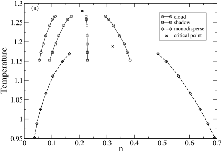
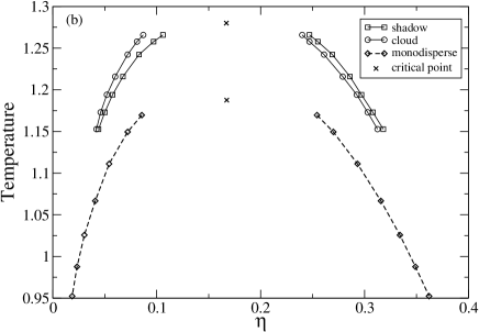
Figure 1: The measured phase diagram of the size-disperse LJ fluid. (a) The $n-T$ representation. (b) The $\eta-T$ representation. In both cases, the phase diagram of the monodisperse limit (broken line) is shown for comparison. Critical points (determined by finite-size scaling) are shown as crosses. Statistical errors do not exceed the symbol sizes.

Having located the critical point, a detailed mapping of the cloud and shadow curves was performed for a large simulation box of volume $V=11390\bar{\sigma}^{3}$. Attention was focused on the distribution of the fluctuating overall number density, $p(n)$. The gas phase cloud point (incipient liquid phase) corresponds to the situation where $p(n)$ is bimodal, but with vanishingly small weight in the liquid peak. Under these conditions, the position of the low density gas peak provides an estimate of the gas phase cloud density, while that of the liquid peak gives the gas phase shadow density. The converse is true for the liquid phase cloud point and its shadow. Determining the cloud and shadow points as a function of temperature yields the cloud and shadow curves. We have tracked the gas and liquid cloud curves (and their shadows) in a stepwise fashion downwards in temperature from the critical point. Histogram extrapolation was employed to negotiate each temperature step, yielding estimates for both the form of $\mu(\sigma)$ on the cloud curve at the next temperature, and the requisite multicanonical weight function.

The resulting phase diagram is shown in fig. 1(a), together with that of the monodisperse LJ fluid, determined in an earlier study WILDING95 . It should be pointed out that while the positions of the peaks in $p(n)$ provide an accurate estimate of cloud and shadow points at low temperatures, this breaks down near the critical point due to finite-size effects WILDING95 . Thus a naive extrapolation of our curves to their intersection point will tend to overestimate the critical temperature. However, our independent determination of the critical point using finite-size scaling methods (as indicated in fig. 1(a)) is considerably more accurate.

The results of fig. 1(a) show a stark separation of the cloud and shadow curves in the $n-T$ plane. Furthermore, the whole phase diagram is considerably shifted with respect to that of the monodisperse fluid. Specifically, one observes that the critical point occurs at a considerably higher temperature than in the monodisperse limit. This particular finding contrasts with that of a previous theoretical study of a size-disperse van-der Waals fluid BELLIER00 , which predicts a suppression of the critical temperature with respect to the monodisperse limit.

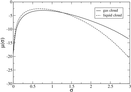
Figure 2: The measured form of the chemical potential distribution $\mu(\sigma)$ at the gas and liquid phase cloud points for $T=0.91T_{c}$. Statistical errors do not exceed the symbol sizes.

The standard order of cloud and shadow curves with increasing density is cloud-shadow-cloud-shadow. By contrast, the pattern apparent in fig. 1(a) is cloud-shadow-shadow-cloud. Interestingly, however, the order reverts to the standard pattern if one plots the data in terms of the volume fraction $\eta=(\pi/6)\int d\sigma\sigma^{3}\rho(\sigma)$, rather than the number density, as shown in fig. 1(b). Moreover, one sees that in the $\eta-T$ representation the differences between cloud and shadow phase properties become much less pronounced. In particular, while the critical number density of the polydisperse fluid is considerably less than its value in the monodisperse limit, the critical volume fraction for the mono- and polydisperse fluid agree to within error. However, irrespective of the choice of data representation, we observe that for our model the critical point occurs very close to the top of the coexistence curve. No clear evidence was discernible for distinct cloud and shadow points, at or above $T_{c}$.

Notwithstanding these intriguing findings, not all differences between gas and liquid cloud points at a given temperature can be camouflaged by a simple change of variable. At temperatures significantly below criticality, we observe dramatic broadening of the coexistence curve in the space of $\mu(\sigma)$. This is shown in fig. 2 which presents the form of $\mu(\sigma)$ at the respective cloud points for the lowest temperature studied, $T=0.91T_{c}$. Such broadening does not occur in monodisperse systems (coexistence occurs at a single value of the chemical potential, not a range of values). The effect is surprisingly large, even given the high degree of polydispersity of the parent ($\delta=40\%$). Indeed, in simulation terms, the respective cloud points are so far separated in phase space that to connect them directly (via a route crossing the phase boundary) required a dozen overlapping simulations–twice as many as were required to connect the cloud point to the critical point at this temperature. We remark in passing that similar aspects of coexistence curve broadening have recently been analyzed within the context of Landau theory by Rascon and Cates RASCON03 .

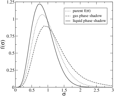
Figure 3: The normalized form of the particle size distribution at the gas and liquid phase shadow points at $T=0.91T_{c}$. The average particle diameter in the gas phase shadow is $\bar{\sigma}=1.167(3)$, while that in the liquid-phase shadow is $\bar{\sigma}=0.863(2)$. Also shown for comparison is the parent shape function $f(\sigma)$, corresponding to the respective cloud phase distributions.

Finally in this section we present the normalized daughter phase distributions at the gas and liquid cloud points for $T=0.91T_{c}$. The data show that at the gas phase cloud point, larger particles preferentially occupy the shadow phase. Conversely at the liquid phase cloud point, there is a predominance of smaller particles in the shadow phase. Clearly the scale of these fractionation effects is considerable: the polydispersity of the gas phase shadow at this temperature is close to $50\%$, while that of the liquid phase shadow is $\approx 33\%$, to be compared with a parent polydispersity of $40\%$.

V Discussion and conclusions

In summary, we have demonstrated how extended sampling grand canonical simulations can be combined with histogram extrapolation methods and a new non-equilibrium potential refinement scheme to accurately determine the phase behaviour of a polydisperse fluid. The results show that in contrast to existing theoretical predictions, the critical temperature of the polydisperse system exceeds that of its monodisperse counterpart. As regards the sub-critical region, we find that the relative order of cloud and shadow curves changes depending on whether the data is represented in terms of the overall number density or the volume fraction. Additionally, we observe considerable polydispersity-induced broadening of the coexistence region: at a given temperature, the cloud points of the respective phases (which coincide in a monodisperse system) are widely separated in terms of their chemical potential distributions. The scale of this effect is mirrored in the disparate forms of the shadow phase daughter distributions.

In a future publication WILDING04 , we will present further simulation results for the magnitude of critical point shifts as a function of the width of the governing size distribution $f(\sigma)$. These results will be compared with those of a moment based theoretical analysis SOLLICH98 ; SOLLICH01 of an improved model free energy for the size disperse van der Waals fluid. The latter correctly captures the sign of polydispersity-induced critical point shifts and provides insights into the deficiencies of previous approaches.

- (1) Larson R.G., The Structure and Rheology of Complex fluids (Oxford University Press, New York, 1999).
- (2) Sollich P., J. Phys. Condens. Matter 14,R79,(2002).
- (3) Evans R.M.L., Fairhurst D.J. and Poon W.C.K., Phys. Rev. Lett. 81, 1326, (1998)
- (4) Fairhurst D.J. and Evans R.M.L., Colloid and Polymer Science (in press), (2004).
- (5) van Heukelum A., Barkema G.T., Edelman M.W., van der Linden E., de Hoog E.H.A.,Tromp R.H.,Macromolecules 36, 6662, (2003).
- (6) Bolhuis P.G., Kofke D.A., Phys. Rev. E59, 618 (1999).
- (7) D.A. Kofke, J. Chem. Phys. 98, 4149, (1993).
- (8) Stapleton M.R., Tildesley D.J., Quirke N., J. Chem. Phys. 92, 4456 (1990).
- (9) Kristóf T., Liszi J., Mol. Phys. 99, 167 (2001).
- (10) Wilding N.B. and Sollich P., J. Chem. Phys. 116, 7116, (2002).
- (11) Escobedo F., J. Chem. Phys. 115, 5642 (2001).
- (12) Wilding N.B., J. Chem. Phys. 119, 12163 (2003).
- (13) Ferrenberg A.M. and Swendsen R.H., Phys. Rev. Lett. 63, 1195 (1989).
- (14) Bruce A.D., Wilding N.B., Adv. Chem. Phys. 127, 1 (2003).
- (15) Berg B. and Neuhaus T., Phys. Rev. Lett.68, 9 (1992).
- (16) Wilding N.B., Phys. Rev. E52, 602 (1995).
- (17) Bellier-Castella L., Xu H. and M. Baus, J. Chem. Phys.113, 8337 (2000).
- (18) Rascón, C., M.E. Cates, J. Chem. Phys 118, 4318 (2003).
- (19) Wilding N.B., Fasolo M. and Sollich P., Unpublished.
- (20) Sollich P. and Cates M.E., Phys. Rev. Lett.80, 1365, (1998)
- (21) Sollich P., Warren P.B., Cates M.E., Adv. Chem. Phys. 116, 265 (2001).