Microscopic dynamics and relaxation processes in liquid Hydrogen Fluoride

Abstract

Inelastic x-ray scattering and Brillouin light scattering measurements of the dynamic structure factor of liquid hydrogen fluoride have been performed in the temperature range$T=214\div 283K$. The data, analysed using a viscoelastic model with a two timescale memory function, show a positive dispersion of the sound velocity $c(Q)$ between the low frequency value $c_{0}(Q)$ and the high frequency value $c_{\infty\alpha}(Q)$. This finding confirms the existence of a structural ($\alpha$) relaxation directly related to the dynamical organization of the hydrogen bonds network of the system. The activation energy $E_{a}$ of the process has been extracted by the analysis of the temperature behavior of the relaxation time $\tau_{\alpha}(T)$ that follows an Arrhenius law. The obtained value for $E_{a}$, when compared with that observed in another hydrogen bond liquid as water, suggests that the main parameter governing the $\alpha$-relaxation process is the number of the hydrogen bonds per molecule.

I Introduction

To understand how the presence of a relaxation process affects the dynamics of the density fluctuations in liquids is one of the open problems in the physics of the condensed matter. Despite the fact that a large effort has been devoted to shed light on this subject, the matter is still under debate. In this respect, among all the relaxations active in a liquid, particular attention has been paid to relaxation processes of viscous nature which strongly affect the longitudinal density modes. They include at least two distinct contributions: a structural (or $\alpha$) and a microscopic (or $\mu$) process. The $\alpha$-process is associated to the structural rearrangement of the particles in the liquid and its characteristic time ($\tau_{\alpha}$) is strongly temperature dependent. $\tau_{\alpha}$ can vary several order of magnitude going from the ps, in the high temperature liquid phase, to $\sim 100~{}s$ in glass-forming materials at the glass transition temperature. The $\mu$-process takes its origin from the oscillatory motion of a particle in the cage of its nearest neighbors before escaping. Its characteristic time $(\tau_{\mu})$ is shorter than $\tau_{\alpha}$ and its ”strength” is often larger than the strength of the $\alpha$-process. Other relaxation processes, beyond the $\alpha$ and the instantaneous processes, associated with the internal molecular degrees of freedom may be observed in molecular liquids Monaco et al. (1999b); Brodin et al. (2002). The existence of the $\alpha$ and $\mu$ processes, already introduced several years ago in a molecular dynamic simulation study on a Lennard-Jones fluid Levesque et al. (1973), has recently been proved by experiments on liquid metals Scopigno et al. (2002a); Scopigno et al. (2001); Scopigno et al. (2000a, b). In this respect another very important class of liquids to consider are the hydrogen bonded (HB) liquid systems. In these compounds indeed, the highly directional hydrogen bond plays a crucial role in the determination of their microscopic properties. Despite the large number of theoretical studies  Honda (2002); Rothlisberger and Parrinello (1997); Jedlovszky and Vallauri (1997a, b); Jedlovszky and Vallauri (1998); Kreitmeir et al. (2003); Bertolini et al. (1998); Balucani et al. (1999, 2000), the way in which the peculiarities of the hydrogen bond networks affect the static organization and the dynamical behavior of these compounds is still a subject of discussion. Many are the parameters related to the hydrogen bond that must be considered in the description of the physical properties of these liquids, as for example the hydrogen bond strength, the spatial network arrangement of the hydrogen bonds and the number of hydrogen bonds per molecule. From an experimental point of view, a study of the collective dynamics as a function of these parameters is extremely important to clarify the role played by each of them on the physical properties of HB systems. Among the HB liquids, hydrogen fluoride (HF) represents one of the most intriguing systems as demonstrated by the large amount of theoretical study on its static  Honda (2002); Rothlisberger and Parrinello (1997); Jedlovszky and Vallauri (1997a, b); Jedlovszky and Vallauri (1998); Kreitmeir et al. (2003) and dynamic  Bertolini et al. (1998); Balucani et al. (1999, 2000) properties. It represents, in fact, a perfect HB model system: it has a simple diatomic molecule and a very strong hydrogen bond that determines a linear chain arrangement of the HB network. Nevertheless, despite its apparent simplicity, only few experimental data are available because of the very high reactivity of the material that consequently makes its handling extremely difficult. In a previous work Angelini et al. (2002) we studied the high frequency dynamics of liquid HF by inelastic x-ray scattering (IXS) at fixed temperature demonstrating the presence of both structural and microscopic relaxation processes. In the present paper we present an extended study of HF as a function of the temperature in the liquid phase between $T_{B}=292~{}K$ the boiling point and $T_{M}=193~{}K$ the melting point. Comparing the results obtained with two different techniques, IXS and Brillouin light scattering (BLS), we find the presence of a structural relaxation process in the entire explored temperature range. The relaxation time $\tau_{\alpha}(T)$, in the sub-picosecond time scale, follows an Arrhenius temperature dependence with an activation energy strictly related to the number of hydrogen bonds. The paper is organized as follow: Sec. II is devoted to the description of the experimental aspects related to the IXS and BLS measurements of the dynamic structure factor of HF. Sec. III is dedicated to the data analysis, in Sec. IV the main results are discussed and finally in Sec. V the outcomes of this study are summarized.

II Sample environment and experimental set-up

High purity (99.9%) hydrogen fluoride has been purchased by Air Products and distilled in the scattering cell without further purification. The sample cell was made out of a stainless steel block, this material is well suited to resist to the chemical reactivity of HF. To allow the passage of the incident and scattered beam, two sapphire windows of $250\mu m$ thickness and $6~{}mm$ diameter, have been glued on two holder plates which have then been screwed to the body of the cell. An o-ring of parofluor has been applied between the window holders and the cell to guarantee a good tightness. The whole cell has been thermoregulated by means of a liquid flux cryostat DC50-K75 Haake. Further details of the sample cell will be described elsewhere Angelini

II.1 Brillouin light scattering experiment

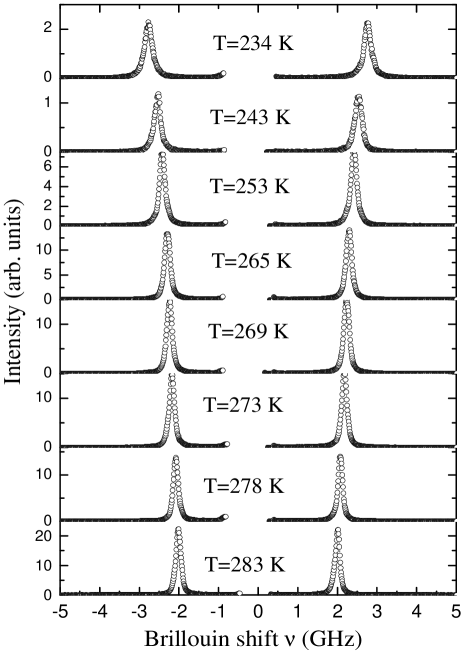
Figure 1: Brillouin light scattering spectra of hydrogen fluoride at the indicated temperatures.

The dynamic structure factor of HF in the GHz range has been measured by Brillouin light scattering using a Sandercock-type multi-pass tandem Fabry-Perot interferometer characterized by high contrast ($>5\cdot 10^{10}$), resolution (FWHM $\approx$ 0.1 GHz) and a finesse of about 100. The wavelength of the incident radiation was $\lambda=514.5nm$ and the light scattered by the sample was collected in the back-scattering geometry ($\theta=180^{0}$). The free spectral range (FSR) was set to 10 GHz, the integration time was approximately $2.5~{}s/channel$. The polarization of the incident light was vertical while the light scattered by the sample was collected in the unpolarized configuration. The aim of the present measurement is to determine the frequency position and width of the Brillouin doublets associated to the propagation of the sound modes. As the relaxation time for HF ,in the investigated temperature range, is in the sub-picosecond region, we do not expect any evidence of the mentioned relaxation processes in the GHz range. Thus from the measured Brillouin peak position and width, it is possible to extract information about the adiabatic sound velocity $c_{0}$ and the kinematic longitudinal viscosity $\nu_{L}$.

II.2 Inelastic x-rays scattering experiment

The inelastic x-rays experiment has been carried out at the very high energy resolution IXS beam-line ID16 at the European Synchrotron Radiation Facility. The instrument consists of a back-scattering monochromator and five independent analyzers operating at the (11 11 11) Si Bragg reflection. They are held one next to the other with a constant angular offset on a 6.5 m long analyzer arm. The used configuration Masciovecchio et al. (1996a), gives an instrumental energy resolution of 1.6 meV full width half maximum (FWHM) and a Q offset of 3 $nm^{-1}$ between two neighbor analyzers. The momentum transfer, Q, is selected by rotating the analyzer arm. The spectra at constant Q and as a function of energy were measured with a Q resolution of $0.4\ \ nm^{-1}$ FWHM. The energy scans were performed varying the back-scattering monochromator temperature with respect to that of the analyzer crystals. Further details on the beam-line are reported elsewhere Masciovecchio et al. (1996b). Each scan took about 180 min and each spectrum at fixed Q was obtained by summing up to 3 or 6 scans.

III Data reduction

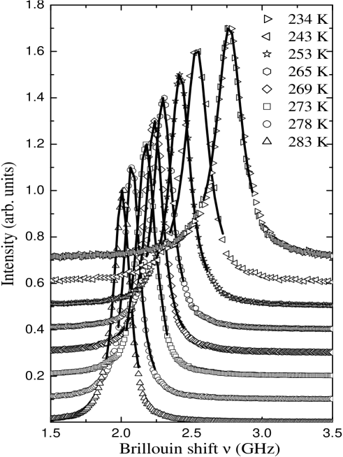
Figure 2: Stokes part of the Brillouin light scattering spectra of HF at the indicated temperatures. The fit (solid line) are superimposed to the data (open symbols). The curves are shifted on the y-axis one respect to the other.

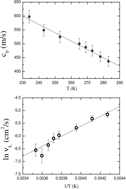
Figure 3: (a) Sound velocity $c_{0}$ and (b) Kinematic longitudinal viscosity $\nu_{L}$ from Table 1 as calculated from the position and the width of the Brillouin light scattering excitations in back-scattering geometry $(\theta=180^{0})$ (full circles). The straight lines represent the linear fit to the data.

III.1 Brillouin light scattering

Unpolarized Brillouin spectra collected in a temperature range between $234~{}K$ and $283~{}K$ are shown in Fig. 1. The quantities of interest are the position and the width of the Brillouin peaks directly related to the sound velocity $c_{0}$ and to the kinematic longitudinal viscosity $\nu_{L}$ of HF. In order to extract these two parameters the experimental data have been fitted in a limited region around the inelastic peaks with the function obtained by the convolution of the instrumental resolution $R(\omega)$ with a damped harmonic oscillator (DHO) function:

$$I(Q,\omega)=R(\omega)\otimes A{{2\Gamma(Q)\Omega(Q)^{2}}\over(\Omega(Q)^{2}-\omega^{2})^{2}+(2\omega\Gamma(Q))^{2}}$$ (1)

where $\Omega=2\pi\nu_{0}$ is the bare oscillation frequency and $2\Gamma$ is approximately the full width at half maximum (FWHM) of the sound excitations. The results of the fitting procedure are reported in Fig. 2 superimposed to the experimental data.

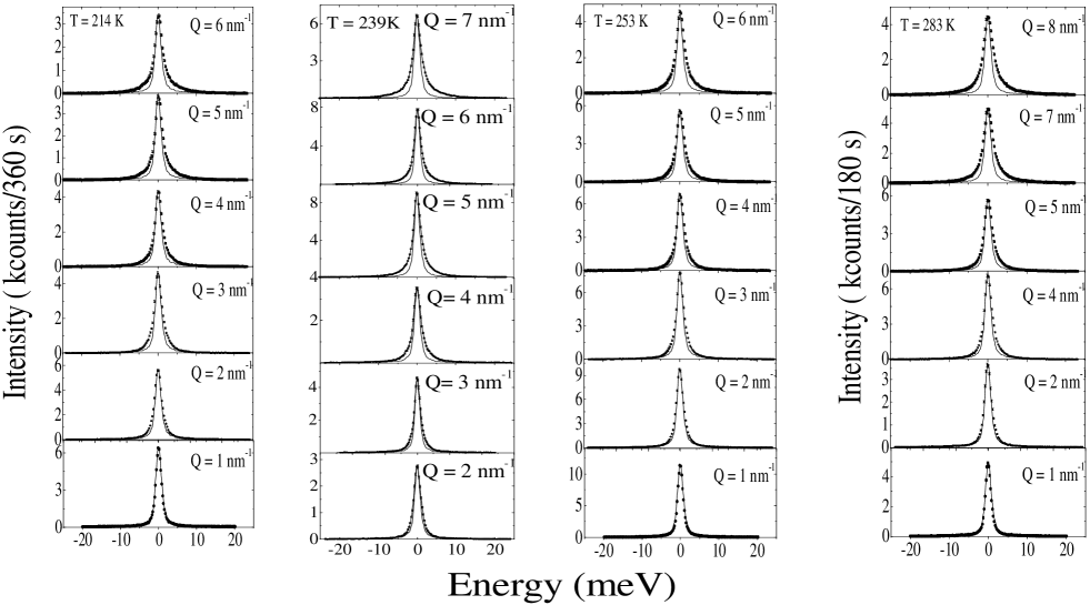
Figure 4: IXS spectra of HF at fixed temperature in the low-Q region. The raw data (lines + symbol) are plotted together with the corresponding experimental resolutions (dashed lines).

Table 1: Values of the frequency position $\nu_{0}$ and of the width $2\Gamma$ of the Brillouin doublet as obtained by the fitting procedure described in the text. The Q values, are also reported together with the sound velocities $c_{0}$ and the kinematic longitudinal viscosities $\nu_{L}$.

T			$\nu_{0}$			$2\Gamma/2\pi$			$Q$		$c_{0}$			$\nu_{L}$
(K)			$(GHz)$			$(GHz)$			$(nm^{-1})$		$(m/s)$			$(cm^{2}/s)$
234			2.74			0.24			0.029		600			0.0058
243			2.51			0.20			0.029		550			0.0049
253			2.39			0.14			0.029		530			0.0034
265			2.27			0.10			0.029		500			0.0026
269			2.21			0.09			0.028		490			0.0023
273			2.15			0.07			0.028		480			0.0017
278			2.05			0.05			0.028		450			0.0011
283			1.97			0.06			0.028		440			0.0014

By exploiting the relations $\Omega(Q)=c_{0}Q$ and $\nu_{L}=2\Gamma/2\pi$, the adiabatic sound velocity $c_{0}$ and the kinematic longitudinal viscosity $\nu_{L}$ are obtained. The exchanged momentum $Q$ values are determined via the relation $Q={4\pi n\over\lambda}sin({\theta\over 2})$, where $n$ is the refractive index and $\theta$ is $180^{0}$ in the used scattering geometry. The temperature dependent refractive index, $n(T)$, has been obtained by using the Clausius-Mossotti relation:

$${n(T)^{2}-1\over n(T)^{2}+2}={4\over 3}\pi\rho_{n}(T)\alpha$$ (2)

where $\rho_{n}$ is the number density and $\alpha$ the optical polarizability of the HF molecule. The latter quantity, $\alpha$, has been obtained using the values of $n(T\approx 293K)$ Lide (1998) and $\rho(T\approx 293K)$ Landolt-Boernestein (1998) and assuming no temperature dependence for this parameter which turns out to be $\alpha=(9.606\pm 0.008)~{}\AA^{3}$. The data for $n(T)$ have then been obtained at each temperature by using $\alpha$ and $\rho(T)$ whose expression is given by  Landolt-Boernestein (1998)

$$\rho(T)=\rho_{0}+A\cdot T$$ (3)

with $\rho_{0}=(1.616\pm 0.003)~{}g/cm^{3}$ and $A=-(2.25\pm 0.01)\cdot 10^{-3}~{}g/cm^{3}K$. The derived values of the sound velocity $c_{0}$ and the kinematic longitudinal viscosity $\nu_{L}$ are reported in Tab. I and shown in Fig. 3. The quantity $c_{0}(T)$ follows a linear behavior characterized by a temperature dependence well represented by the equation:

$$c_{0}(T)=c_{0}+B\cdot T$$ (4)

with $c_{0}=(1290\pm 40)~{}m/s$ and $B=(-3.0\pm 0.1)~{}m/sK$. The same procedure has been applied to derive the kinematic longitudinal viscosity $\nu_{L}$ for which the linear fit provides a temperature behavior described by the relation:

$$ln\nu_{L}(T)=C+{D\over T}$$ (5)

with $C=(-13.5\pm 0.7)~{}cm^{2}/s$ and $D=(1960\pm 170)~{}cm^{2}K/s$. All the values of Q, of the fit parameters and of the calculated $\nu_{L}$ and $c_{0}$, are reported in Table 1.

III.2 Inelastic x-rays scattering

The IXS measurements, performed to probe the dynamics of HF in the mesoscopic regime, are compared to the BLS results of the previous section in order to characterize the transition from the hydrodynamic regime to the mesoscopic. In this case the $S(Q,\omega)$ has been studied at four temperatures in the range 214-283 K at T = 214 K, T = 239 K, T = 254 K and T = 283 K as a function of the wave vector Q. It has been varied between $1\div 15nm^{-1}$ for all the studied temperatures excepted for T = 239 K, where it has been selected between $2\div 31nm^{-1}$. Each energy scan took 180 min and each spectrum at fixed Q was obtained by summing up to 6 or 3 scans. We report in Fig. 4 an example of the measured spectra at the investigated temperatures and at the indicated momentum transfer (dotted line); they are compared with the instrumental resolution aligned and scaled to the central peak (full line).

III.2.1 Markovian approach

Figure 5: Dispersion curves at the indicated temperatures. The upper full lines are the linear fits to the high-Q data. The lower dashed lines indicate the adiabatic sound velocity as measured by Brillouin light scattering as shown in Sec. II.1.

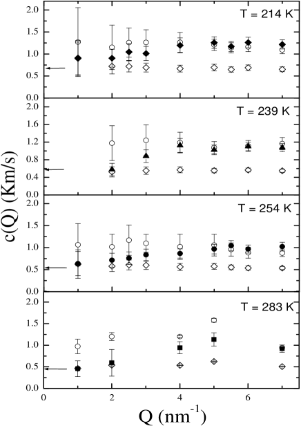
Figure 6: Q-dependence of the sound velocities $c_{0}(Q)$ (open diamonds) and $c_{\infty\alpha}(Q)$ (open circles) from a viscoelastic analysis, together with $c(Q)$ (full symbols) from Fig. 5. The value of the adiabatic sound velocity, $c_{0}$, is indicated by the arrow.

A first raw analysis of the spectra has been done in terms of the Markovian approximation in the memory function approach Balucani and Zoppi (1994). In this approach the $S(Q,\omega)$ is expressed as:

$$S(Q,\omega)=I(Q){{\omega_{0}(Q)}^{2}M^{\prime}(Q,\omega)\over[\omega^{2}-\omega_{0}(Q)^{2}-\omega M^{\prime\prime}(Q,\omega)]^{2}+[\omega M^{\prime}(Q,\omega)]^{2}}$$ (6)

where $\omega_{0}(Q)^{2}=(K_{B}T/mS(Q))Q^{2}$ is the normalized second frequency moment of $S(Q,\omega)$, $K_{B}$ is the Boltzmann constant, $m$ is the mass of the molecule and $M^{\prime}(Q,\omega)$, $M^{\prime\prime}(Q,\omega)$ are respectively the real and the imaginary part of the Laplace transform of the memory function $M(Q,t)$. In the Markovian approximation, the decay of the memory function is faster than any system time scale and is modelled with a $\delta$ function in the time domain Balucani and Zoppi (1994) in such a way that Eq. 6 reduces to a DHO. To fit our data we used this function plus a Lorentzian to take into account the finite width of the quasi elastic central peak . The detailed balance and the convolution with the instrumental resolution have also been taken into account during the fitting procedure. One of the parameters we are interested in, is $\Omega(Q)$ which corresponds to the frequency of the sound modes. Its dispersion curve (i.e. its Q-dependence)is shown in Fig. 5 at low $Q$ for the four analysed temperatures. The data show a common behaviour in the entire investigated T range, namely a linear dependence in the $Q$ range $4-5\div 7~{}nm^{-1}$, with a slope corresponding to sound velocities higher than the adiabatic values $c_{o}$ measured by BLS and reported in the previous section. In addition for lower Q, the apparent sound velocity $c(Q)$ determined by IXS seems to show a transition from the low frequency value $c_{o}$ to the higher value. This result provides the necessary information to extend what recently observed in liquid HF at $T=239~{}K$ Angelini et al. (2002) to a wider temperature range. The increase of $c(Q)$ with increasing Q, in fact, is interpreted as due to the presence of a relaxation process, the structural relaxation, already observed in HF at $T=239~{}K$ and still present in the whole explored temperature region.

III.2.2 Viscoelastic approach

Figure 7: Q-dependence of the relaxation times $\tau_{\alpha}(Q)$ from the viscoelastic analysis at the indicated temperatures. A constant fit in the low Q region (dashed line) is also reported.

Figure 8: Q-dependence of the parameter $\Gamma_{\mu}(Q)$ (full circles) in liquid HF at the analyzed temperatures from a viscoelastic analysis. The full lines are the parabolic fits to the low-Q data.

The existence of a relaxation process with a characteristic time $\tau$ in the range of the probed sound waves (i.e. such that $\Omega\tau\simeq 1$), as evident from the dispersion of $\Omega(Q)$, calls for a more refined choice of the memory function with respect to the Markovian approximation. To describe the effect of this relaxation in $S(Q,\omega)$, we use the memory function based on the viscoelastic model. In this approach we describe a two relaxation process scenario with a memory function $M(Q,t)$ given by the sum of an exponential decay contribution and a $\delta$-function Angelini et al. (2002) :

$$M(Q,t)=\Delta_{\alpha}^{2}(Q)e^{-{t/\tau_{\alpha}(Q)}}+\Gamma_{\mu}(Q)\delta(t)$$ (7)

where $\Delta_{\alpha}^{2}(Q)=[c_{\infty\alpha}(Q)^{2}-c_{0}(Q)^{2}]Q^{2}$, is the strength of the $\alpha$ process and $\Gamma_{\mu}(Q)=\Delta_{\mu}^{2}\tau_{\mu}(Q)$. As in pure HF at $T=239~{}K$ Angelini et al. (2002) in fact, one expects a structural process described by an exponential decay and a microscopic process, very fast respect to the investigate time scale Monaco et al. (1999a) described by a $\delta-$function. This approach has been successfully applied in the past to describe the dynamics of simple liquids Cunsolo et al. (2001) and liquid metals Scopigno et al. (2002b, a); Scopigno et al. (2001); Scopigno et al. (2000a, b). The thermal contribution in the memory function has been neglected being the value of the specific heats ratio $\gamma$ close to 1. The experimental data have been fitted to the convolution of the experimental resolution function with the dynamic structure factor model given by the combination of Eq. 6 and 7.

The Q dependence of the fit parameters $c_{\infty\alpha}(Q)$, $c_{0}(Q)$, $\tau_{\alpha}(Q)$ and $\Gamma_{\mu}(Q)$ is described in the following .

In Fig. 6 the Q behavior of the sound velocities is shown in the low Q region and for all the investigated temperatures. Both he infinite $c_{\infty\alpha}(Q)$ and zero $c_{0}(Q)$ frequency limiting values, as obtained from the viscoelastic fit, are reported (open symbols). The comparison with the apparent sound velocity $c(Q)=\Omega(Q)/Q$ (full symbols) as derived from the dispersion curve of Fig. 5, shows the transition of c(Q) from $c_{0}(Q)$ to $c_{\infty\alpha}(Q)$. The consistency between the two independent analysis strongly suggests that this transition is governed by the $\alpha$-relaxation process in the entire temperature range.

The Q dependence of the relaxation time $\tau_{\alpha}(Q)$ is reported in Fig. 7 at the four investigated temperatures and in the $Q$ range $1\div 15~{}nm^{-1}$. It shows a constant behavior, within the error bars, in the low Q region and a very week decrease at increasing Q as already observed in water Monaco et al. (1999a) and many other systems Balucani and Zoppi (1994). The fit of the data in the $1\div 7~{}nm^{-1}$ range yields values $\tau_{\alpha}(Q\rightarrow 0)$ reported in Tab. 2. In Fig. 8 the Q dependence of the strength of the microscopic relaxation, $\Gamma_{\mu}(Q)$, is reported at the four analyzed temperatures. The data show a quadratic behavior and have been fitted with a parabolic function

$$\Gamma_{\mu}(Q)=DQ^{2}$$

The values of the parameter $D$ are reported in Tab 2 as a function of the temperature.

Figure 9: (a) Behavior of the sound velocities in $HF$ as a function of the temperature : $c_{0}$ (open squares), $c_{\infty\alpha}$ (open circles). (b) Sound velocities ratio $c_{\infty\alpha}/c_{0}$ (symbols); the straight line represents a constant fit to the data.

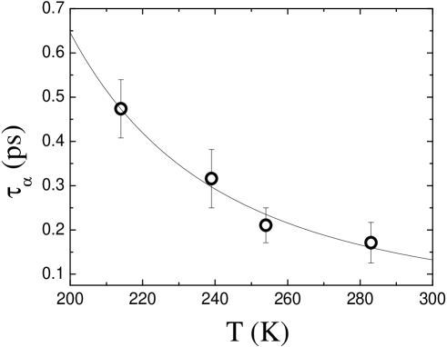
Figure 10: T dependence of the low-Q extrapolation of the relaxation times $\tau_{\alpha}(Q)$ of Figure 7 together with the Arrhenius fit (full line) of Eq. 8.

Table 2: Low Q values of the parameters used to calculate the kinematic longitudinal viscosity $\nu_{L}(0)$ of Eq. 9: $c_{0}(0)$ from Eq. 4; $c_{\infty\alpha}(0)$ from the linear fit of Fig. 5; $\tau(0)$ and $\Gamma$ derived from the viscoelastic analysis as described in the text.

T			$c_{0}(0)$			$c_{\infty\alpha}(0)$			$\tau_{\alpha}(0)$			$D$			$\nu_{L}(0)$
$(K)$			$(m/s)$			$(m/s)$			$(ps)$			$(cm^{2}/s)$			$(cm^{2}/s)$
214			650			1220			0.47			0.0030			0.007
239			580			1080			0.32			0.0022			0.004
254			530			1010			0.21			0.0026			0.003
283			480			980			0.17			0.0026			0.003

IV Discussions

This section is dedicated to the discussion of the temperature dependence of the low Q behavior of the different parameters analysed in the previous paragraphs. These parameters fully characterize the collective dynamics of our system in the mesoscopic regime. The values of $c_{0}$, $c_{\infty\alpha}$ and $c_{\infty\alpha}/c_{o}$ at the four investigated temperatures are reported in Fig. 9. As shown in Fig. 9(b) the ratio $c_{\infty\alpha}/c_{o}$ is temperature independent in all the explored T-range and it is close to two as in the case of water Sette et al. (1996). The temperature dependence of the structural relaxation time in the $Q\rightarrow 0$ limit has been deduced from Fig. 7. Here the low $Q$ part of $\tau_{\alpha}(Q)$ has been fitted using a constant function. The obtained values are reported in Fig. 10 on a linear scale as a function of the temperature. In the explored temperature range, the $\tau_{\alpha}(T)$ behavior is well described by the Arrhenius law (full line):

$$\tau_{\alpha}(T)=\tau_{0}e^{{E_{a}\over K_{B}T}}$$ (8)

with an activation energy $E_{a}=(1.9\pm 0.2)~{}kcal/mol$ and $\tau_{0}=(6\pm 2)10^{-15}s$. The temperature dependence in the limit $Q\rightarrow 0$ of the last fit parameter $D$ is reported in Tab. 2. It yields values which appear to be temperature independent being $D=(0.170\pm 0.025)~{}meV/nm^{-2}=(2.6\pm 0.4)\cdot 10^{-3}~{}cm^{2}/s$. This result is consistent with previous findings according to which the microscopic relaxation is a temperature independent process Monaco et al. (1999a). Using the low Q values $\tau_{\alpha}(0)$ of Tab. 2 together with the low Q extrapolations of the other parameters (see Tab. 2), it is possible to calculate the kinematic longitudinal viscosity $\nu_{L}$ from the relation Balucani and Zoppi (1994):

$$\nu_{L}=\tau_{\alpha}({0})(c_{\infty\alpha}^{2}(0)-c_{0}^{2}(0))+{D\over 2Q^{2}}$$ (9)

where $c_{0}$ is the adiabatic sound velocity measured by Brillouin light scattering as discussed in previous section. The derived values for $\nu_{L}$ are reported in Fig. 11: they are found to be consistent with the hydrodynamic data reported in Tab. 1 . This equivalence gives further support to the validity of the employed viscoelastic model. In the same figure we also report two viscosity data determined by molecular dynamics (MD) simulation simulations. A recent MD study of the transport coefficients (longitudinal and shear viscosity, thermal diffusivity and conductivity) of hydrogen fluoride Balucani et al. (2000) provides two values for the longitudinal viscosity $\eta_{L}$, one at $T=205K$, $\eta_{L}(T=205K)=0.91\cdot 10^{-2}g/cms$ and the other at $T=279K$, $\eta_{L}(T=279K)=0.38\cdot 10^{-2}g/cms$. They are reported in Fig. 11 after rescaling for the density of Eq. 3 according to the relation $\nu_{L}(T)=\eta_{L}(T)/\rho(T)$, they are quite consistent with the experimental data.

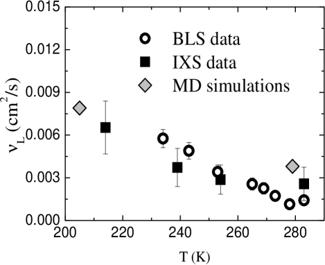
Figure 11: Temperature dependence of the kinematic longitudinal viscosity: from IXS as calculated through Eq. 9 (full squares), from the Brillouin light scattering values of Table 1 (open circles) and from molecular dynamic simulations at $T=205K$ and $T=279K$ (full diamonds) Balucani et al. (2000).

Figure 12: Arrhenius plot for the relaxation time as obtained from viscoelastic analysis of the dynamical structure factor for water (diamonds) Monaco et al. (1999a) and hydrogen fluoride (circles); The dashed lines indicate the best linear fit to the data and their slop give an activation energy of $3.8~{}kcal/mol$ for water and $1.9~{}kcal/mol$ for HF.

In Fig. 12 we report, on an Arrhenius plot, the comparison between the relaxation times for hydrogen fluoride and for water Monaco et al. (1999a). The activation energy found in water, constant in the examined temperature range, was $E_{a}=(3.8\pm 0.6)~{}kcal/mol$ while the one for hydrogen fluoride is $E_{a}=(1.9\pm 0.2)~{}kcal/mol$ as previously discussed. It is worthwhile to relate the values of the activation energies to the different networks present in the two liquids. While hydrogen fluoride forms linear chains with one hydrogen bond on average for each molecule, the preferred arrangement of water is the three-dimensional tetraedric structure with two hydrogen bonds for each molecule. If we indicate with $n_{HB-H_{2}O}$ and $n_{HB-HF}$ the number of hydrogen bonds for $H_{2}O$ and $HF$ respectively and $E_{a-H_{2}O}$, $E_{a-HF}$ the activation energies for the two liquids, we see that they satisfy the ratio:

$${E_{a-H_{2}O}\over n_{HB-H_{2}O}}\approx{E_{a-HF}\over n_{HB-HF}}$$ (10)

In previous studies on water Montrose et al. (1974) the activation energy has been associated with that of the H-bond $(\approx 5kcal/mol)$ Pauling (1939). The result of Eq. 10 strengthens the idea that the structural relaxation process involves the H-bond networks of the system and it seems also to suggest that in this case the activation energy of the process is related to the number of H-bonds to make and break and not only to the strength of each H-bond.

V Conclusions

We have presented inelastic Brillouin light and inelastic x-rays scattering measurements of liquid hydrogen fluoride, a prototype of the class of hydrogen bonded liquid systems, in a temperature range comprised between $214~{}K$ and $283~{}K$. We demonstrated that the collective dynamics of liquid HF is characterized by a structural relaxation process in the sub-picosecond time scale. In the explored temperature region this relaxation process affects the collective dynamics in a Q range between $1\div 7nm^{-1}$. An accurate analysis in terms of the viscoelastic model in the memory function approach allowed to extract and determine the temperature dependence of the parameters describing the dynamics at microscopic level. The relaxation time related to the structural relaxation process follows an Arrhenius temperature behavior with an activation energy $E_{a}$ which, compared with the value previously measured in liquid water, enables to establish a connection between $E_{a}$ and the number of hydrogen bonds per molecule of the specific system.