Finite spin-glass transition of the $\pm J$ XY model in three dimensions

Abstract

A three-dimensional $\pm J$ XY spin-glass model is investigated by a nonequilibrium relaxation method. We have introduced a new criterion for the finite-time scaling analysis. A transition temperature is obtained by a crossing point of obtained data. The scaling analysis on the relaxation functions of the spin-glass susceptibility and the chiral-glass susceptibility shows that both transitions occur simultaneously. The result is checked by relaxation functions of the Binder parameters and the glass correlation lengths of the spin and the chirality. Every result is consistent if we consider that the transition is driven by the spin degrees of freedom.

I Introduction

Random and/or frustrated systems exhibit a variety of exotic phenomena. Common knowledge of uniform systems may not be applied to these systems. Randomness sometimes brings order to disorder. Exotic states may appear in the ground state. New-type phase transitions occur in these systems. They are referred to as complex systems and have been attracting wide interest.

Spin glasses SGReview are prototype of complex systems. Ferromagnetic interaction and antiferromagnetic interaction are randomly distributed in the materials. There is frustration in local interaction bonds. Magnetic spins cannot always minimize the interaction energy. They freeze at low temperatures while pointing random directions. This freezing is called the spin-glass transition.

Theoretical investigations on spin glasses are mainly made into the Edwards-Anderson modelEdwards . Spins are located on a regular lattice but the interaction bonds between spins are randomly distributed. Many theoretical methods have been developed. By progress of computational facilities numerical simulations are recently performed. However, simulations in spin glasses suffer from serious slow dynamics. It takes a long time to realize equilibrium states at low temperatures. A numerical method overcoming this difficulty can be successfully applied to other complex systems. One example is an application of the temperature-exchange Monte Carlo methodhukuexchange to protein folding problemsokamoto1 .

Not many problems have been made clear due to the difficulty of simulations in spin glasses. One unsolved problem is whether or not a theoretical model with short-range interaction bonds can explain the real spin-glass transition. There is a general consensus that the spin-glass transition occurs in the Ising model in three dimensions.Bhatt ; Ogielski ; KawashimaY The estimated critical exponents agree with the corresponding experimental resultsAruga . Spins of many spin-glass materials are of Heisenberg type. The Heisenberg spin-glass model in three dimensions should exhibit the spin-glass transition. However, numerical investigations McMillan ; Olive ; Morris concluded that there is no spin-glass transition in this model. There has been discrepancy between theory and experiment in this model.

There are three major theories explaining this discrepancy. One is the anisotropy theory. There are finite magnetic anisotropies in exchange interactions in real materials. Even though there is no spin-glass order in the isotropic Heisenberg model, the spin-glass transitions in real materials are explained by finite anisotropy. Matsubara et al. showed that the anisotropy reinforces the spin-glass order.Matsubara The second theory is the chirality mechanism introduced by Kawamura.KawamuraH1 ; HukushimaH It is argued that there occurs the chiral-glass transition without the spin-glass transition. Finite anisotropy in real materials mixes the chiral degrees of freedom and the spin degrees of freedom. This mixture links the chirality and the spin. The spin-glass transitions in real materials are driven by this chiral-glass transition. This scenario is based on that there is no spin-glass transition in the isotropic model. Since the chirality is defined by spin variables, the chiral-glass transition trivially occurs if the spin-glass transition occurs. Therefore, it is crucial to check whether both transitions occurs at the same temperature or not. The third theory argues a possibility of this simultaneous transition. Matsubara et al. Matsubara3 ; Matsubara4 ; Endoh2 showed several lines of evidence that the spin-glass transition occurs at a finite temperature. Nakamura et al. Nakamura ; Nakamura2 investigated the model by a nonequilibrium relaxation method Stauffer ; Ito ; ItoOz1 ; OzIto2 ; Shirahata2 and obtained the consistent results. Here, we note that nonequilibrium relaxation of the spin-glass susceptibilityHuse and that of the Binder parameterBlundell are known to exhibit the algebraic divergence at the spin-glass transition temperature in the Ising model. Lee and Young Lee also concluded a single chiral-glass and spin-glass transition in the model with Gaussian random bond distributions. These results suggest that the previous investigations which concluded no spin-glass transition have some technical problems.

The situation is same in the XY spin-glass model in three dimensions. Spins are restricted to point in the XY plane in this model. A domain-wall energy analysis Morris and a Monte Carlo simulation analysis Jain concluded no spin-glass transition. The chirality mechanism was originally proposed in this model.KawamuraXY1 ; KawamuraXY2 ; KawamuraXY3 However, a possibility of the finite spin-glass transition has been suggested by recent investigations Lee ; Maucourt ; Kosterlitz ; Granato ; yamamotoissp .

In this paper we focus on the problem in the XY spin-glass model in three dimensions: whether or not the spin-glass transition and the chiral-glass transition occur at the same temperature. It is also made clear why there has been the discrepancy even though investigating the same theoretical model with similar methods. We consider the following three points as origins of the discrepancy. One is ambiguity in the scaling analysis. The obtained results are sometimes dependent on a temperature range of data used in the analysis. We introduce a new scaling criterion to eliminate this ambiguity. The second point is strong effects from system sizes and boundary conditions. We carefully observe how these effects appear in the relaxation data. It is found that the effects are very strong and strange. The third point is a use of the spin-glass susceptibility and the Binder parameter in the equilibrium simulations on finite lattices. Both quantities are under the strong influence of the size effects. These points are discussed in this paper.

The present paper is organized as follows. Section II describes the present model and our method. A new scaling procedure is explained with an example of the ferromagnetic Ising model in two dimensions. Section III shows our results. A finite-time-scaling analysis on the glass susceptibility is performed. The results are confirmed by relaxation functions of the Binder parameter and the glass correlation lengths. Section IV is devoted to summary and discussions.

II Model and Method

II.1 Model and physical quantities

A model we consider in this paper is the $\pm J$ random bond XY model in a simple cubic lattice. The Hamiltonian is given by

$${\cal H}=-\sum_{\langle ij\rangle}J_{ij}\mbox{\boldmath$S$}_{i}\cdot\mbox{\boldmath$S$}_{j}=-\sum_{\langle ij\rangle}J_{ij}\cos{(\theta_{i}-\theta_{j})},$$ (1)

where the sum runs over all the nearest-neighbor spin pairs $\langle ij\rangle$. Each spin, $S$, is defined by angle, $\theta_{i}$, in the XY plane: $\mbox{\boldmath$S$}_{i}=(\cos\theta_{i},\sin\theta_{i})$. The angle $\theta_{i}$ takes continuous values in $[0,2\pi)$, but we divide it to 1024 discrete states in this paper. Effects of the discreteness are checked to be negligible by comparing data of 1024-state simulations with those of 2048-state simulations. The interactions $J_{ij}$ take two values of $+J$ and $-J$ with the same probability. The temperature $T$ is scaled by $J$. Linear lattice sizes are denoted by $L$. Total number of spins is $N=L\times L\times(L+1)$, and skewed periodic boundary conditions are imposed. Spins are updated by the single-spin-flip algorithm using the conventional Metropolis probability.

Physical quantities observed in our simulations are the spin-glass susceptibility $\chi_{\mathrm{sg}}$, the chiral-glass susceptibility $\chi_{\mathrm{cg}}$, the Binder parameters $g_{\mathrm{sg}}$ and $g_{\mathrm{cg}}$, the glass correlation length $\xi_{\mathrm{sg}}$ and $\xi_{\mathrm{cg}}$. The spin-glass susceptibility is defined by the following expression.

$$\chi_{\mathrm{sg}}\equiv\frac{1}{N}\left[\sum_{i,j}\langle\mbox{\boldmath$S$}_{i}\cdot\mbox{\boldmath$S$}_{j}\rangle^{2}\right]=\frac{2N}{m(m-1)}\left[\sum_{A>B,\mu,\nu}(q_{\mu,\nu}^{AB})^{2}\right]$$ (2)

The subscripts $\mu$ and $\nu$ denote two components, $x$ and $y$, of spin variables $S$. The thermal average is denoted by $\langle\cdots\rangle$, and the random-bond configurational average is denoted by $[\cdots]$. The thermal average is replaced by an average over independent real replicas: $\langle\cdots\rangle\to(1/m)\sum_{A}^{m}$. Replica number is denoted by $m$. Superscripts $A$ and $B$ are the replica indices. The number $m$ determines resolution of the thermal average. It should be large in order to improve the accuracy of average. We prepare 32 replicas ($m=32$) with different initial spin configurations in this paper. Each replica is updated in parallel with a different random number sequence. An overlap between two replicas is defined by

$$q_{\mu\nu}^{AB}\equiv\frac{1}{N}\sum_{i}{S}_{i\mu}^{(A)}{S}_{i\nu}^{(B)}.$$ (3)

The chiral-glass susceptibilityKawamuraXY2 is similarly defined by

$$\chi_{\mathrm{cg}}\equiv\frac{6N}{m(m-1)}\left[\sum_{A>B}(q_{\kappa}^{AB})^{2}\right],$$ (4)

where

$$q_{\kappa}^{AB} \equiv \frac{1}{3N}\sum_{\alpha}\,{\kappa}_{\alpha}^{(A)}{\kappa}_{\alpha}^{(B)},$$ (5)

$$\kappa_{\alpha}^{(A)} \equiv \frac{1}{2\sqrt{2}}\sum_{\langle jk\rangle\in\alpha}J_{jk}\sin{(\theta_{j}^{(A)}-\theta_{k}^{(A)})}.$$ (6)

A local chirality variable, $\kappa_{\alpha}^{(A)}$, is defined at each square plaquette $\alpha$ that consists of the nearest-neighbor bonds $\langle jk\rangle$.

The Binder parameters for the spin glass and for the chiral glass are calculated through the following expressions. Here, we have also replaced the thermal averages by the average over real replicas.

$$g_{\mathrm{sg}} = 3-2\left(\frac{\sum\limits_{\mu,\nu,\delta,\rho}\left[\frac{2}{m(m-1)}\sum\limits_{A>B}^{m}(q_{\mu\nu}^{AB})^{2}(q_{\delta\rho}^{AB})^{2}\right]}{\sum\limits_{\mu,\nu}\left[\frac{2}{m(m-1)}\sum\limits_{A>B}^{m}(q_{\mu\nu}^{AB})^{2}\right]}\right)$$ (7)

$$g_{\mathrm{cg}} = \frac{1}{2}\left(3-\frac{\left[\frac{2}{m(m-1)}\sum\limits_{A>B}^{m}(q_{\kappa}^{AB})^{4}\right]}{\left[\frac{2}{m(m-1)}\sum\limits_{A>B}^{m}(q_{\kappa}^{AB})^{2}\right]}\right)$$ (8)

Since the Binder parameters lose size dependences at the transition temperature, the nonequilibrium relaxation functions exhibit algebraic divergence with an exponent $d/z$.Blundell From the exponent we can obtain a value of the dynamic exponent $z$. It also serves as another check of the spin-glass transition. If the susceptibility and the Binder parameter exhibit algebraic divergence, it is very certain that the phase transition occurs. Kawamura and Li KawamuraXY3 argued that the Binder parameter of the chiral glass shows a negative dip at the transition temperature. They observed crossing behavior of the Binder parameter on the negative side. We observe nonequilibrium relaxation of the Binder parameter in order to check this negative crossing: it should diverge algebraically on the negative side.

A spin-glass correlation function is defined by the following expression.

$$f_{\mathrm{sg}}(l) \equiv \left[\sum_{i}^{N}\langle\mbox{\boldmath$S$}_{i}\cdot\mbox{\boldmath$S$}_{i+l}\rangle^{2}\right]$$

$$= \left[\frac{2}{m(m-1)}\sum_{A>B,i,\mu\nu}q_{\mu\nu}^{AB}(i)q_{\mu\nu}^{AB}(i+l)\right]$$

A length between two spins is denoted by $l$. Here, $q_{\mu\nu}^{AB}(i)=S_{i,\mu}^{(A)}S_{i,\nu}^{(B)}$ is a spin overlap on the $i$ site. A chiral-glass correlation function is defined by the following.

$$f_{\mathrm{cg}}(l)=\left[\frac{2}{3m(m-1)}\sum_{A>B}\sum_{\alpha}q_{\kappa}^{AB}(\alpha)q_{\kappa}^{AB}(\alpha+l)\right]$$ (10)

Here, $q_{\kappa}^{AB}(\alpha)=\kappa_{\alpha}^{(A)}\kappa_{\alpha}^{(B)}$ is a local overlap of the chirality. We only consider a distance $l$ between two parallel square plaquettes. We estimate a spin-glass correlation length $\xi_{\mathrm{sg}}$ and a chiral-glass correlation length $\xi_{\mathrm{cg}}$ fitting the correlation functions by the following expression.

$$f_{\mathrm{sg/cg}}(l)\sim\frac{1}{l^{d-\gamma/\nu}}\exp\left(-\frac{l}{\xi_{\mathrm{sg/cg}}}\right)$$ (11)

Exponent $d$ is a dimension of the lattice ($d=3$), $\gamma$ is the glass susceptibility exponent and $\nu$ is the glass correlation length exponent.

II.2 Nonequilibrium relaxation method

We start simulations from random spin configurations. This is a paramagnetic state at $T=\infty$. The temperature is quenched to a finite value from the first Monte Carlo step. At each step we observe physical quantities and obtain the relaxation functions. Changing an initial spin state, a random bond configuration, and a random number sequence we start another simulation and obtain another set of the relaxation functions. We take averages of relaxation functions over these independent Monte Carlo simulations. The relaxation functions of the susceptibility and the Binder parameter multiplied by $N$ exhibit algebraic divergence at the transition temperature: $\chi_{\mathrm{sg/cg}}\propto t^{\gamma/z\nu}$ and $g_{\mathrm{sg/cg}}\times N\propto t^{d/z}$. A relaxation function of the correlation length also diverges algebraically as $\xi_{\mathrm{sg/cg}}\propto t^{1/z}$. We try to find such a temperature first observing raw relaxation functions. If a temperature is higher than the transition temperature, the susceptibility converges to a finite value even in the infinite-size system. The lowest temperature at which the relaxation data exhibit the converging behavior is the upper bound for the transition temperature.

The second method to estimate the transition temperature is the finite-time scaling analysis OzIto2 . This is a direct interpretation of the conventional finite-size scaling analysis by considering the dynamic scaling hypothesis: $\tau\sim\xi^{z}$. A term “size” is replaced by a term “time” by this relation. We collect relaxation functions of the spin-glass susceptibility at various temperatures. They should fall onto a single universal curve if we properly choose the transition temperature, $T_{\mathrm{sg}}$, and critical exponents, $\gamma$ and $z\nu$. The following equation is the scaling formula.

$$\chi_{\mathrm{sg}}(t)t^{-\gamma/z\nu}=\tilde{\chi}_{\text{sg}}(t/\tau(T)),~{}~{}\tau(T)\propto(T-T_{\mathrm{sg}})^{-z\nu}$$ (12)

Here, $\tilde{\chi}$ denotes a universal scaling function. Monte Carlo step $t$ is scaled by correlation time $\tau(T)$ which diverges algebraically at the transition temperature. We plot data of the spin-glass susceptibility multiplied by $t^{-\gamma/z\nu}$ against $t/(T-T_{\mathrm{sg}})^{-z\nu}$. An estimation of the chiral-glass transition temperature is performed by the same procedure.

At the estimated transition temperature we observe relaxation functions of the Binder parameter and the correlation length. They should exhibit algebraic divergence. The observation supports the occurrence of the transition. The dynamic exponent $z$ is estimated by these relaxation functions. The exponent of the Binder parameter is $d/z$ and that of the correlation length is $1/z$. We can check consistency of the estimates comparing these two values.

II.3 New criterion for scaling analysis

Finite-size/time-scaling analysis is a powerful tool to investigate critical phenomena. The method has been applied to various systems successfully. However, it sometimes has ambiguity obtaining correct values of the transition temperature and the critical exponents. One example is a spin-glass transition problem in the $\pm J$ Heisenberg model in three dimensions. Olive et al. Olive performed a finite-size-scaling analysis of the spin-glass susceptibility and concluded that the phase transition does not occur. Matsubara et al.Matsubara4 reported in the preprint version that the same analysis may give a finite transition temperature. A difference of these two analyses is a temperature range of data used in the scaling. We also experience this kind of ambiguity in the present paper.

Determination of good scaling is usually done by the looks of scaling plots. All the scaled data are fitted by some polynomial functions. One which makes the least standard deviation is selected to be the best scaling result. It may change if we use a different set of temperature/size/time ranges in the analysis. This change is systematic.

For example, we consider a situation when a ratio of exponents $\gamma/z\nu$ in Eq. (12) is larger than the correct value. The left-hand-side of the scaling formula becomes smaller and smaller as time increases. This tendency is stronger at lower temperatures where the correlation time is relatively large. In order to make scaled data fall onto a single curve we must choose $\tau(T)$ at lower temperatures to be smaller than the correct values. This is because the universal scaling function $\tilde{\chi}$ is a decreasing function with respect to $t/\tau(T)$. Since $\tau(T)\propto(T-T_{\mathrm{sg}})^{-z\nu}$, the transition temperature is underestimated when a ratio $\gamma/z\nu$ is larger than the correct value. As we discard data at higher temperatures and restrict our analysis to lower temperature ranges, the transition temperature is more and more underestimated. Contrarily, the transition temperature is more and more overestimated when the ratio $\gamma/z\nu$ is smaller than the correct value. When the ratio is correct, the correct transition temperature is obtained and the value is robust against changes of the temperature range.

Our new criterion for the scaling is to find a temperature and critical exponents so that the obtained results are independent from the temperature range of data used in the scaling analysis. First, we set one temperature range. We obtain the transition temperature which gives the best scaling plot at each point of $\gamma/z\nu$. The obtained transition temperature is plotted against $\gamma/z\nu$. Changing the temperature range we perform the same analysis and obtain another plot for the transition temperature. These plots exhibit systematic behavior as mentioned above. They cross at one point, which is the most probable estimate for the transition temperature.

Figure 1 shows an example of the analysis with the new scaling criterion in the ferromagnetic Ising model in two dimensions. The lattice size is $499\times 500$ with skewed periodic boundary conditions. The Monte Carlo step is 2400. The first 300 steps are discarded, which contain initial relaxation. Simulations are performed at nineteen different temperatures ranging $2.276\leq T\leq 2.35$. Averages over 124000 independent Monte Carlo runs are taken. When a ratio $\gamma/z\nu$ is larger, estimates of the transition temperature go down as the temperature range shrinks to lower temperatures. They go up when a ratio is smaller. The plots cross near the exact point. Deviation from the exact value is larger for the exponent $z\nu$ as shown in Fig. 1(b). Crossing behavior is rough in this case. An estimation of the exponent is difficult compared to the transition temperature. We perform this scaling procedure to estimate the spin-glass transition temperature and the chiral-glass transition temperature.

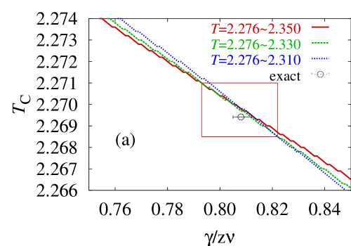
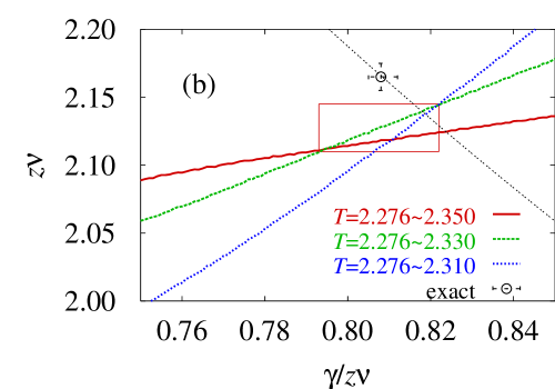
Figure 1: Results of the finite-time-scaling analysis with our new criterion in a ferromagnetic Ising model in two dimensions. An exact estimate using $z=2.165(10)$ 2dising is depicted by a symbol. Boxes depict error bars. (a) $T_{\mathrm{c}}$ versus $\gamma/z\nu$. (b) $z\nu$ versus $\gamma/z\nu$. A thin line is an exact line regardless a value of $z$.

III Results

III.1 Relaxation of the susceptibility

First, we observe raw relaxation functions of the glass susceptibility. We must check time scale when the finite-size effects appear in the relaxation functions. Data must be free from the finite-size effects because the nonequilibrium relaxation method is based upon taking the infinite-size limit before the equilibrium limit is taken. The susceptibility data influenced by the size effects exhibit converging behavior even though it should diverge in the infinite-size limit. It misleads us into thinking that the temperature is in the paramagnetic phase.

Figure 2 shows the appearance of the finite-size effects of $\chi_{\mathrm{sg}}(t)$ and $\chi_{\mathrm{cg}}(t)$. When a size is small, a nonequilibrium relaxation function deviates from the size-independent relaxation curve at a characteristic time. The system finds itself finite at this time. It behaves as an infinite-size system before the time. There is no difference between data of $L=39$ and those of $L=49$. Therefore, relaxation functions of $L=39$ within $t\leq 10^{5}$ are regarded as of the infinite-size system. We mainly use this set of size and time limits in this paper. Number of random bond configurations is typically more than several hundreds. It varies depending on system sizes, Monte Carlo steps, and physical quantities. For example, quite a few configurations are necessary in order to obtain beautiful relaxation functions for the Binder parameter and the correlation length.

It is also noted in Fig. 2 that behavior of the finite-size effects of the chiral-glass susceptibility is opposite to the spin-glass one. The spin-glass susceptibility deviates from the diverging curve just to converge to a finite value. It is natural behavior. On the other hand, the chiral-glass susceptibility increases when the size effects appear. It eventually converges to a finite value and is overtaken by the infinite-size one. This strange behavior is also observed in the $\pm J$ Heisenberg model in three dimensions.Nakamura

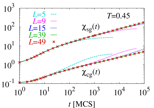
Figure 2: Finite-size effects of relaxation functions of $\chi_{\mathrm{sg}}(t)$ and $\chi_{\mathrm{cg}}(t)$. The temperature $T=0.45$ is near our estimate for the transition temperature. There is no size dependence for $L=39$ within $10^{5}$ Monte Carlo step.

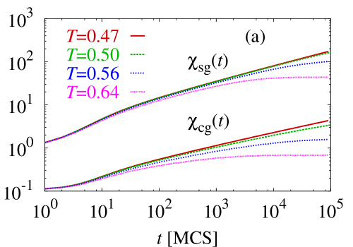
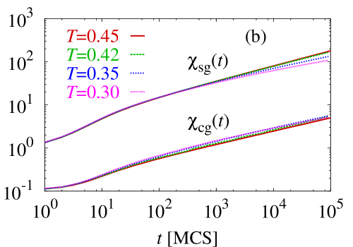
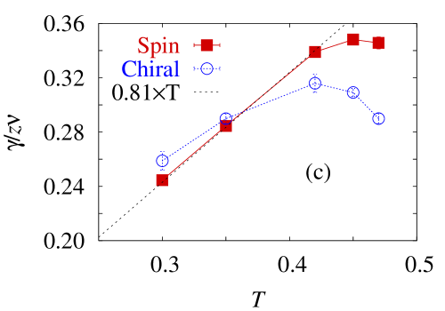
Figure 3: Relaxation functions of $\chi_{\mathrm{sg}}$ and $\chi_{\mathrm{cg}}$ at various temperatures. (a) Plots at $T\geq 0.47$: high temperature side. (b) Plots at $T\leq 0.45$: low temperature side. (c) Exponents of algebraic divergence in $\chi_{\mathrm{sg}}$ and $\chi_{\mathrm{cg}}$ at lower temperatures.

Figure 3(a) shows relaxation functions of $\chi_{\mathrm{sg}}(t)$ and $\chi_{\mathrm{cg}}(t)$ for $T\geq 0.47$. This is a plot on the high temperature side. It is clear that there is no spin-glass/chiral-glass transition at $T>0.50$. Both susceptibility exhibit converging behavior. They exhibit algebraic divergence at $T=0.47$. It suggests that the spin-glass transition occurs at a temperature near $T=0.47$. Figure 3(b) shows a plot at lower temperatures. The spin-glass susceptibility diverges algebraically with exponents decreasing with the temperatures. The exponent is largest at $T=0.45$. We consider it to be near the transition temperature. The same behavior is observed in the $\pm J$ Ising model in three dimensions below the spin-glass transition temperature.Komori ; totaIsing Slow dynamics appear in the low-temperature spin-glass phase. Relaxation of the glass susceptibility may become algebraically slow. The chiral-glass susceptibility also exhibit algebraic divergence at lower temperatures. The amplitude as well as the exponent is dependent on the temperatures.

Temperature dependences of the exponents are shown in Fig. 3(c). Algebraic divergence starts appearing at $T\sim 0.47$. An exponent of the spin-glass susceptibility takes a maximum value near $T=0.45$. It is considered in the vicinity of the transition temperature. The exponent decreases as the temperature decreases. This temperature dependence is linear with $T$:

$$\gamma/z(T)\nu=0.81T,~{}~{}1/z(T)\sim 0.4T.$$ (13)

Here, we have used our final estimate for a ratio $\gamma/\nu=2.0(2)$ obtained in Sec. III.4. The temperature dependence of $1/z$ in the Ising model with Gaussian bond distributions is reported by Komori et al. Komori to be $1/z(T)=0.17T$. The low-temperature phase in the present XY model is similar to that of the Ising model.

Temperature dependences of an exponent of the chiral-glass susceptibility is strange compared with the spin-glass one. The algebraic divergence begins at $T=0.47$. As the temperature decreases, the exponent first increases and takes a maximum value at $T=0.42$ and then decreases with temperature. The temperature of the maximum exponent is lower than that of the spin-glass one.

From the relaxation functions of the susceptibility it is very possible that the spin-glass phase transition occurs at $T=0.45\pm 0.03$. The chiral-glass transition also occurs within this temperature range. Since the chirality trivially freezes if the spin freezes, these two transitions may occur simultaneously. The low-temperature relaxation functions of the spin-glass susceptibility exhibit a property of the spin-glass phase: an inverse of the dynamic exponent is linearly dependent on the temperature. We check these findings performing the finite-time scaling analysis. Stress is put upon consistency of a transition temperature and a ratio of critical exponents $\gamma/z\nu$ at that temperature.

III.2 Finite-time-scaling analyses

We perform a finite-time-scaling analysis with our new criterion. Figures 4(a) and 4(b) show results of the scaling on the spin-glass transition. For each value of $\gamma/z\nu$ we choose $T_{\mathrm{sg}}$ and $z\nu$ so that fitting error of the scaled data becomes smallest. The fitting is done by a polynomial expression up to the 7th order. Relaxation data of the first two thousand steps are discarded. We considered them to be the initial relaxation. The scaling results are dependent on the temperature range. The dependence is also as described in Sec. II.1: when $\gamma/z\nu$ is larger, the transition temperature becomes underestimated as high temperature data are discarded, and vice versa. From the crossing point we obtain our estimates as

$$T_{\mathrm{sg}} = 0.455\pm 0.015$$ (14)

$$\gamma/z\nu = 0.355\pm 0.005$$ (15)

$$z\nu = 4.8\pm 0.4.$$ (16)

Figure 4(c) shows a scaling plot using the obtained results. All data fall onto a single scaling function very nicely. The obtained transition temperature is higher than other estimates. Granato Granato gave $T_{\mathrm{sg}}=0.39(2)$, $\nu=1.2(2)$ and $z=4.4(3)$. A value of $z\nu$ is consistent with our value. Lee and Young Lee gave for the Gaussian model $T_{\mathrm{sg}}=0.34(2)$ and $\nu=1.2(2)$. Our estimate for $\nu$ is $\nu=0.85(15)$, where we use a value of $z$ which will be obtained in Sec. III.4 (Eq. (20)). Though the transition temperature is quite different, critical exponents are consistent.

Values of $T_{\mathrm{sg}}$ and $\gamma/z\nu$ obtained by the scaling analysis agree with the relaxation function of the susceptibility in the previous subsection. As shown in Fig. 3(c) an exponent of the spin-glass susceptibility takes a maximum value at around $T=0.45$ and the exponent is $\gamma/z\nu=0.348$. Both values are consistent with the scaling results. A scaling estimation of $T_{\mathrm{sg}}=0.4$ is possible if we artificially choose $\gamma/z\nu$ and the temperature range of the data used in the scaling analysis. An example is a set of choices: $\gamma/z\nu=0.366$ and $T=0.50\sim 0.56$ as shown in Fig. 4(a) with circles. However, it is inconsistent with the relaxation functions of the spin-glass susceptibility. It does not diverge with an exponent $\gamma/z\nu=0.366$ at $T=0.4$. Only the scaling results that are independent from the temperature ranges (a crossing point in the figure) become consistent with the raw relaxation functions.

Figures 5(a), 5(b) and 5(c) shows results on the chiral-glass transition. Estimations of the transition temperature and critical exponents are

$$T_{\mathrm{cg}} = 0.467\pm 0.010$$ (17)

$$\gamma_{\kappa}/z_{\kappa}\nu_{\kappa} = 0.30\pm 0.01$$ (18)

$$z_{\kappa}\nu_{\kappa} = 4.7\pm 0.2.$$ (19)

Subscripts $\kappa$ of the critical exponents denote chirality. Kawamura and Li gave $T_{\mathrm{cg}}=0.39(3)$, $\nu_{\kappa}=1.2(2)$, $\gamma_{\kappa}/\nu_{\kappa}=1.85(20)$, and $z_{\kappa}=7.4(10)$. Our estimation for the transition temperature is higher than their value. We will obtain a value of $z_{\kappa}=6.3(5)$ from a relaxation function of the chiral-glass correlation length in Sec. III.4. Then, an exponent $\nu_{\kappa}=0.75(10)$ is obtained. This value is also smaller than their value. However, a ratio of exponents, $\gamma_{\kappa}/\nu_{\kappa}=1.9(2)$, is consistent. As observed in Fig. 3(c) an exponent $\gamma_{\kappa}/z_{\kappa}\nu_{\kappa}$ of the chiral-glass susceptibility takes a maximum value of $\gamma_{\kappa}/z_{\kappa}\nu_{\kappa}=0.315$ at $T=0.42$. This temperature is consistent with the estimation of Kawamura and Li. However, this set of $T$ and $\gamma_{\kappa}/z_{\kappa}\nu_{\kappa}$ is inconsistent with the scaling results of Fig. 5(a). To the contrary, our scaling estimations are consistent with the relaxation functions of the chiral-glass susceptibility. We consider that the chiral-glass transition occurs at $T\sim 0.47$. Algebraic divergence begins at this temperature. The temperature of the exponent maximum does not correspond to the transition temperature of the chirality.

The spin-glass transition temperature and the chiral-glass transition temperature agree well within the error bars. Therefore, both transitions are considered to occur simultaneously. Estimations are consistent with the raw relaxation functions. The consistency guarantees that our analyses are performed correctly.

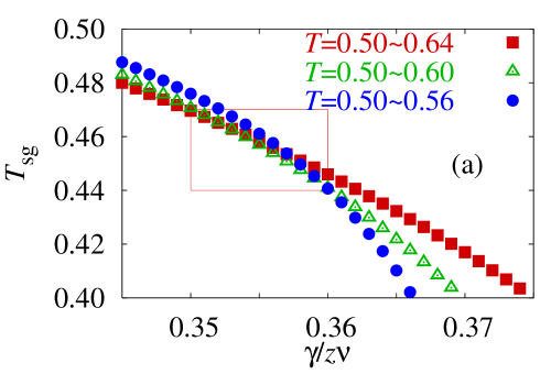
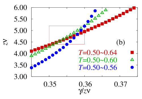
Figure 4: Results of the present finite-time-scaling analysis on the spin-glass transition. (a) $T_{\mathrm{sg}}$ versus $\gamma/z\nu$. (b) $z\nu$ versus $\gamma/z\nu$. (c) A scaling plot using the obtained parameters.

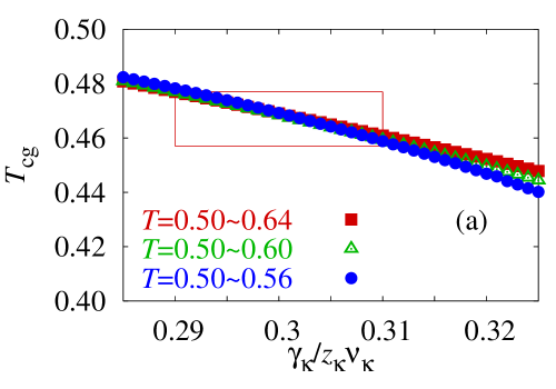
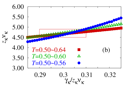
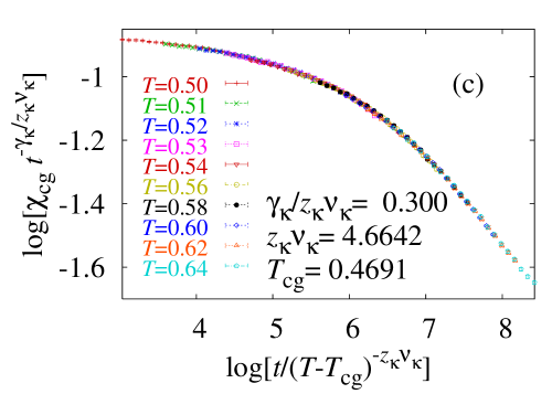
Figure 5: Results of the present finite-time-scaling analysis on the chiral-glass transition. (a) $T_{\mathrm{sg}}$ versus $\gamma/z\nu$. (b) $z\nu$ versus $\gamma/z\nu$. (c) A scaling plot using the obtained parameters.

III.3 Relaxation of the Binder parameter

In order for another check of our scaling results and for obtaining the dynamic exponent $z$ independently we have calculated the nonequilibrium relaxation functions of the Binder parameter at the estimated transition temperature.

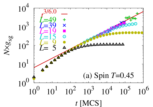
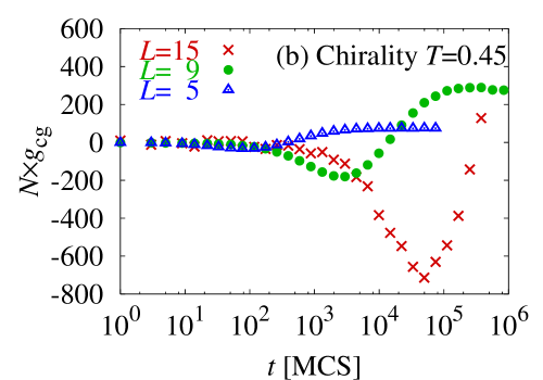
Figure 6: Relaxation functions of the Binder parameters at $T=0.45$. (a) A log-log plot for the spin-glass one. Algebraic divergence is observed. (b) A semi-log plot for the chiral-glass one. No divergence is observed. When the size effects appear, the Binder parameters take negative values first and converge to positive values.

Figure 6(a) shows relaxation functions of the Binder parameter of the spin, $g_{\mathrm{sg}}(t)$, for various system sizes. When a size is small, a relaxation function deviate from the size-independent relaxation curve. Appearance of the finite-size effect is normal as in the case of the spin-glass susceptibility. It just converges to a finite value when the size effect appears. The size-independent curve exhibits an algebraic divergence with an exponent $d/z$ with $z\sim 6.0\pm 0.5$. We have also obtained the relaxation functions at $T=0.42$ and $T=0.47$. (Figures not shown in this paper.) These temperatures are within the error bar of the spin-glass transition temperature. The algebraic divergence of the Binder parameter is also observed. It is noted that the dynamic exponent $z$ is systematically dependent on the temperature. The values are $z=6.5\pm 0.7$ at $T=0.42$ and $z=5.7\pm 0.5$ at $T=0.47$. They are consistent with the temperature dependence of $z$ in Eq. (13): $1/z(T)\sim 0.4T$ within error bars. The dynamic exponent is estimated to be $z=6.0\pm 0.8$ within an error bar of the spin-glass transition temperature.

Relaxation functions of the Binder parameter of the chiral-glass shows strange behavior. The algebraic divergence as in the spin-glass one cannot be observed at all in Fig. 6(b). A value of the Binder parameter remains zero before the finite-size effects appear. Then, it decreases and takes negative values. Taking a minimum value it increases with time and eventually converges to a positive value, which is consistent with a result of Kawamura and LiKawamuraXY3 . This strange finite-size effect possibly has the same origin with that of the chiral-glass susceptibility as shown in Fig. 2. The chiral-glass Binder parameter is considered to take zero value at $T>T_{\mathrm{cg}}$ in the infinite-size system.

III.4 Relaxation of the correlation length

In this subsection the final check is made on our analysis concerning the spin-glass transition. We also answer questions and claims regarding use of the nonequilibrium relaxation method in spin-glass problems.

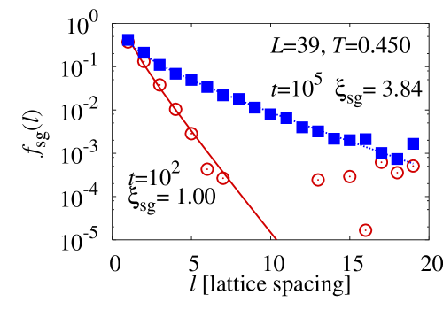
Figure 7: Estimations of a correlation length $\xi_{\mathrm{sg}}(t)$ by fitting a correlation function $f_{\mathrm{sg}}(l)$. Data at $t=10^{2}$ are depicted by circles and those at $t=10^{5}$ are depicted by squares.

Figure 7 shows the spin-glass correlation functions at Monte Carlo steps $t=10^{2}$ and $t=10^{5}$. The temperature is near the spin-glass transition temperature. We have taken averages over three directions, $x$, $y$ and $z$, between spins. The distance is limited within $L/2$ because we have imposed skewed periodic boundary conditions. Our simulations start from the perfectly random spin configuration. There is no correlation between spins and the correlation length is zero at $t=0$. The spin-glass correlation grows with time. The correlation decays fast at $t=10^{2}$ but decay is slow at $t=10^{5}$. We estimate the correlation length fitting the correlation functions by an expression Eq. (11). Here, we have set $\gamma/\nu=2.4$. We obtain a ratio of $\gamma/\nu\simeq 2.1(3)$ from the scaling result of $\gamma/z\nu=0.355(5)$ together with an estimate of the dynamic exponent $z=6.0(8)$ by the Binder parameter. We performed the fitting with several values of $\gamma/\nu$ in this range. Amplitudes of the correlation lengths change with $\gamma/\nu$. When a value of $\gamma/\nu$ is small, $\xi_{\mathrm{sg}}$ is overestimated: it becomes 40% larger if we set $\gamma/\nu=1.8$. However, the dynamic-scaling behavior, $\xi\sim t^{1/z}$, and the exponent $z$ remain the same. We discard data of the correlation functions which are lower than $10^{-3}$ in the fitting procedure. This is resolution of the present simulations. Numerical data may take negative values below this resolution limit even though the definition Eq. (II.1) demands positive values. The obtained correlation length is not influenced by such garbage data. The spin-glass correlation length at $t=10^{2}$ is $\xi_{\mathrm{sg}}=1.00$, and $\xi_{\mathrm{sg}}=3.84$ at $t=10^{5}$. The growth is very slow. We have also obtained the chiral-glass correlation length in the same manner.

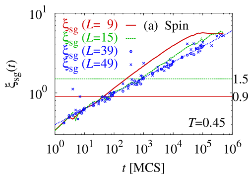
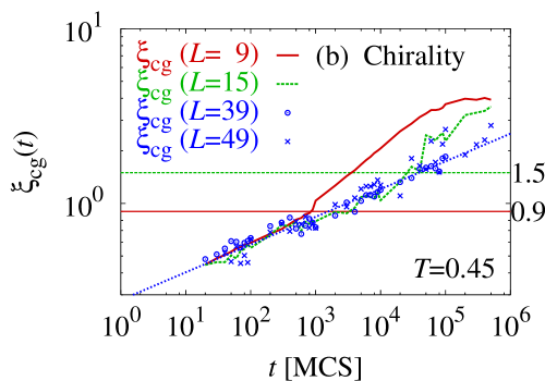
Figure 8: Relaxation functions of (a) the spin-glass correlation length and (b) the chiral-glass correlation length. Linear sizes of lattices are denoted by $L$. Fitting lines for the size-independent data are $\xi_{\mathrm{sg}}(t)=0.4t^{1/5.1}$ and $\xi_{\mathrm{cg}}(t)=0.3t^{1/6.3}$, respectively. The size effect appears when the correlation length reaches $L/10$ in every case.

Figure 8 shows relaxation functions of the spin-glass correlation length and the chiral-glass correlation length. At each Monte Carlo step we calculate the correlation functions and obtain the correlation lengths. The correlation length exhibits algebraically diverging behavior until $t=10^{6}$. There is no size dependence between data of $L=39$ and those of $L=49$. We can regard them the infinite-size data. Random configuration number of the $L=39$ data is 235, and that of the $L=49$ data is 122. Deviations from the fitting line are larger for the $L=49$ data. The dynamic exponent of the spin-glass correlation length is $z=5.1\pm 0.5$. This value is a little smaller than the estimation by the Binder parameter, which gave $z=6.0\pm 0.8$. Both estimates are independent. Thus, we take an average of them and obtain our final estimate.

$$z = 5.6\pm 0.6~{}~{}~{}(\mathrm{spin})$$ (20)

$$z_{\kappa} = 6.3\pm 0.5~{}~{}~{}(\mathrm{chirality})$$ (21)

Using the value of spin and $\gamma/z\nu=0.355(5)$ we obtain a ratio of the critical exponents of the spin-glass susceptibility as $\gamma/\nu=2.0(2)$.

It is remarkable that the spin-glass correlation length starts the diverging behavior almost from the first step. A correlation length is about 0.5 lattice spacings. The chiral-glass correlation length also starts the diverging behavior at $t=50$ where a correlation length is also 0.5 lattice spacings. This is a characteristic length above which we can observe the algebraic divergence of the correlation length. It is considered to be determined by resolution of simulations. The figure also shows how the finite-size effects appear in the relaxation functions of the correlation lengths. In both plots the finite-size effects appear when the correlation lengths reach $L/10$. We have observed the size effect at other temperatures. It also appears when $\xi\sim L/10$.

The size effects enhance the correlation length. The skewed periodic boundary conditions are imposed in this paper. Boundary effects produce correlation of a spin with itself. Therefore, the correlation is always overestimated by the size effects. Then, the correlation length is also overestimated. The spin-glass correlation length of $L=9$ reaches $\xi_{\mathrm{sg}}=6$ in the equilibrium limit as shown in Fig. 8(a). In a lattice of $L=9$ the largest distance is $L/2=4.5$. The correlation length exceeds this limit. Therefore, such a value does not have a physical meaning at all. This is a consequence of the size effect. One may think that the size effect appears when the correlation length reaches the system size. However, it appears when $\xi$ reaches $L/10$. Finite-size effects are very strong in spin glasses. We must pay much attention to the size effects on numerical data.

These lines of evidence may answer the question why the nonequilibrium relaxation method can handle the spin-glass problems. Relaxation processes in the scaling region know the critical phenomenon from the very early time steps. There is a characteristic length that we can observe the critical behavior. This is $\xi=0.5$ lattice spacings in the present simulations. This length is surprisingly small. This is because resolution of our simulations is very sharp. It is an advantage of the nonequilibrium relaxation method. Critical relaxation continues until the finite-size effects appear. It is a time when $\xi$ reaches $L/10$. If the temperature is off the transition temperature, critical relaxation continues until the correlation length reaches its equilibrium finite value at the temperature. What is slow in spin glasses is a relaxation process after the finite-size effects appear. For example, $\xi_{\mathrm{sg}}$ of $L=9$ in Fig. 8(a) deviate from the size-independent line at $t\sim 30$. It reaches the equilibrium limit at $t=10^{5}$. Computations before this time are discarded in the equilibrium simulations. On the other hand, those before the size effects appear ($t\sim 30$) are utilized in the nonequilibrium relaxation method. Therefore, the critical phenomenon of spin glasses is easily observed if we take the nonequilibrium relaxation approach. Another advantage of this approach is that the system size can be considered infinity. The size effects are very strong and strange in spin glasses as shown in this paper. We can get rid of these effects by this method. These are the reasons why the nonequilibrium relaxation method is successful in the spin-glass problems.

IV Summary and Discussion

In this paper we made clear that the simultaneous spin-glass and chiral-glass transition occurs in the $\pm J$ XY model in three dimensions. We have eliminated ambiguity of the scaling analysis by introducing a new criterion: correct results are independent of the temperature range of data used in the scaling. The results are checked and confirmed by the relaxation functions of the spin-glass susceptibility, the Binder parameter and the spin-glass correlation length. They are consistent with each other. The evaluated transition temperature is higher than other estimations,Lee ; Granato while the critical exponents are consistent.

The transition temperature of the spin-glass transition and that of the chiral-glass transition agree well within the error bars. A ratio of the static critical exponents, $\gamma/\nu$, takes almost the same value between two. They are $\gamma/\nu=2.0(2)$ for the spin and $\gamma_{\kappa}/\nu_{\kappa}=1.9(2)$ for the chirality. This agreement suggests that two transitions are qualitatively equivalent. The dynamic exponent $z$ of the spin-glass obtained by the Binder parameter and that obtained by the correlation length becomes consistent when $T_{\mathrm{sg}}=0.47$. This temperature is an upper bound of the error bar and is very close to the mean value of the chiral-glass transition temperature.

The spin-glass susceptibility and the Binder parameter exhibit normal behavior of the second-order phase transition. Both exhibit algebraic divergence at the transition temperature. An exponent of the divergence is strongest at the transition temperature. Contrarily, those of the chiral-glass transition show strange behavior. The chiral-glass susceptibility diverges algebraically at the transition temperature. However, an exponent of the susceptibility takes a maximum value at a lower temperature. Relaxation of the Binder parameter shows no divergence. It just remains zero in the infinite-size system. If the transition is driven by the chirality degrees of freedom, the Binder parameter should exhibit a kind of critical behavior as the spin-glass one exhibits. Relaxation functions of the chiral-glass correlation length exhibit the same behavior as the spin-glass one. They begin the algebraic divergence when $\xi_{\mathrm{sg/cg}}\sim 0.5$ lattice spacings and stop it at $\xi_{\mathrm{sg/cg}}\sim L/10$ when the finite-size effects appear. The size effects appear later in the chiral-glass because $\xi_{\mathrm{cg}}<\xi_{\mathrm{sg}}$. Kawamura and LiKawamuraXY3 commented that the spin-chiral separation occurs at $T=T_{\mathrm{cg}}$ at $t=10^{5}$ Monte Carlo steps in the standard Metropolis dynamics. We have carried out simulations up to $t=10^{6}$ steps and found no sign of the separation in behaviors of the infinite-size system.

The lines of evidence can be explained if one considers that the glass transition is driven by the spin degrees of freedom. The chirality is defined by spin variables. It trivially freezes if the spin freezes. A critical property may be observed by some quantities of the chirality, but it may not in other quantities. The former example is the chiral-glass susceptibility and the latter one is the Binder parameter. This is because the chirality is the secondary degrees of freedom in this phase transition. Every analysis and the results are consistent in the spin-glass transition. This is a strong support for our argument that the transition is driven by the spin.

The present analyses are based upon numerical simulations. The results always have error bars. We cannot prove that the spin-glass transition temperature is exactly same with the chiral-glass one. Our estimations for the transition temperatures agree within error bars. However, the mean value of the chiral-glass transition temperature is a little larger. In order to make a distinction between two transition temperatures we must carry out simulations 400000 times as large as the present ones. The estimation is as follows. If the mean values are correct, $\chi_{\mathrm{sg}}(t)$ should exhibit converging behavior when $T=0.467$, while $\chi_{\mathrm{cg}}(t)$ remains diverging. We observed converging behavior of $\chi_{\mathrm{sg}}(t)$ at $t=10^{4}$ when $T=0.56$ as shown in Fig. 3(a). Therefore, the converging behavior is observed at $t=3.3\cdot 10^{8}$ when $T=0.467$ because $\tau\propto(T-0.455)^{-4.8}$. The size effects appear when $\xi\sim L/10$ and $\xi_{\mathrm{sg}}(t)=0.4t^{1/5.6}$. Then, a linear lattice size $L=130$ is necessary to obtain size-independent data until $t=3.3\cdot 10^{8}$. Therefore, $3.3\cdot 10^{3}\times(130/39)^{3}\simeq 400000$ times larger simulations are necessary. It is almost impossible to make the distinction by raw relaxation functions.

Why the spin-glass transition has not been observed until quite recently? The first reasonable answer we consider is strong finite-size effects. As shown in Fig. 8 the size effects appear when the correlation length reaches $L/10$. Physically-meaningful spin-glass correlation functions are restricted within this length scale. Those outside this scale are plagued by the size effects. Since the susceptibility collects all the correlation functions, it is also under the strong influence of the size effects. Most of information extracted from the susceptibility may be unphysical one if the lattice size is small. Observations of the spin-glass susceptibility by equilibrium simulations with small lattices may suffer from this difficulty. The second reason is the boundary conditions. Most simulations employ the periodic boundary conditions. They may produce a domain-wall spin state, or a spiral spin state in continuous spin models. Particularly, when the system possesses frustration, nontrivial states may be produced. On the other hand, the nonequilibrium relaxation method achieves the infinite-size system. The obtained data are always independent of the finite-size effects and the boundary conditions. True physical properties are easily extracted.

Recently, the spin-glass transitions are observed by a finite-size scaling analysis on the spin-glass correlation length.Lee The quantity is considered to be less influenced by the size effects. In the present paper we have also obtained relaxation functions of the correlation length. It is evaluated directly from the correlation functions. Unphysical garbage data of correlations are not contained in our estimations. Therefore, the spin-glass transition is clearly exhibited. It is also found that the correlation length exhibits critical behavior from the first step. Analyses on the correlation length will become a standard approach in the spin glass problems.

- (1) For reviews, K. Binder and A. P. Young, Rev. Mod. Phys. 58, 801 (1986); J. A. Mydosh, Spin Glasses (Taylor & Francis, London, 1993) ; Spin Glasses and Random Fields edited by A. P. Young (World Scientific, Singapore, 1997).
- (2) S. F. Edwards and P. W. Anderson, J. Phys. F 5, 965 (1975).
- (3) K. Hukushima and K. Nemoto, J. Phys. Soc. Jpn. 65, 1604 (1996).
- (4) Y. Sugita and Y. Okamoto, Chem. Phys. Lett. 314, 141 (1999).
- (5) R. N. Bhatt and A. P. Young, Phys. Rev. Lett. 54, 924 (1985).
- (6) A. T. Ogielski and I. Morgenstern, Phys. Rev. Lett. 54, 928 (1985).
- (7) N. Kawashima and A. P. Young, Phys. Rev. B 53, R484 (1996).
- (8) K. Gunnarsson, P. Svedlindh, P. Nordblad, L. Lundgren, H. Aruga and A. Ito, Phys. Rev. B 43, 8199 (1991).
- (9) W. L. McMillan, Phys. Rev. B 31, 342 (1985).
- (10) J. A. Olive, A. P. Young and D. Sherrington, Phys. Rev. B 34, 6341 (1986).
- (11) B. W. Morris, S. G. Colborne, M. A. Boore, A. J. Bray and J. Canisius, J. Phys. C 19, 1157 (1986).
- (12) F. Matsubara and T. Iyota and S. Inawashiro, Phys. Rev. Lett. 67, 1458 (1991).
- (13) H. Kawamura, Phys. Rev. Lett. 68, 3785 (1992).
- (14) K. Hukushima and H. Kawamura, Phys. Rev. E 61, R1008 (2000).
- (15) F. Matsubara, S. Endoh and T. Shirakura, J. Phys. Soc. Jpn. 69, 1927 (2000).
- (16) F. Matsubara, T. Shirakura and S. Endoh, cond-mat/0011218; Phys. Rev. B 64, 092412 (2001).
- (17) S. Endoh, F. Matsubara and T. Shirakura, J. Phys. Soc. Jpn 70, 1543 (2001).
- (18) T. Nakamura and S. Endoh, J. Phys. Soc. Jpn. 71, 2113 (2002).
- (19) T. Nakamura, S. Endoh and T. Yamamoto, J. Phys. A 36, 10895 (2003).
- (20) D. Stauffer, Physica A 186, 197 (1992).
- (21) N. Ito, Physica A, 192, 604 (1993).
- (22) N. Ito and Y. Ozeki, Int. J. Mod. Phys. 10, 1495 (1999).
- (23) Y. Ozeki and N. Ito Phys. Rev. B 68, 054414 (2003).
- (24) T. Shirahata and T. Nakamura, Phys. Rev. B 65, 024402 (2001).
- (25) D. A. Huse, Phys. Rev. B 40, 304 (1989).
- (26) R. E. Blundell, K. Humayun, and A. J. Bray, J. Phys. A: Math. Gen. 25, L733 (1992).
- (27) L. W. Lee and A. P. Young, Phys. Rev. Lett. 90, 227203 (2003).
- (28) S. Jain and A. P. Young, J. Phys. C 19, 3913 (1986).
- (29) H. Kawamura and M. Tanemura, J. Phys. Soc. Jpn. 60, 608 (1991).
- (30) H. Kawamura, Phys. Rev. B 51, 12398 (1995).
- (31) H. Kawamura and M. S. Li, Phys. Rev. Lett. 87, 187204 (2001).
- (32) J. Maucourt and D. R. Grempel, Phys. Rev. Lett. 80, 770 (1998).
- (33) J. M. Kosterlitz and N. Akino, Phys. Rev. Lett. 82, 4094 (1999); N. Akino and J. M. Kosterlitz, Phys. Rev. B 66, 054536 (2002).
- (34) E. Granato, J. Magn. Magn. Mater. 226, 364 (2001); E. Granato, Phys. Rev. B 69, 012503 (2004).
- (35) T. Yamamoto and T. Nakamura, ISSP Supercomputer Center Activity Report 2002 (The University of Tokyo, 2003) p. 203.
- (36) N. Ito, Physica A 192, 604 (1993).
- (37) T. Komori, H. Yoshino and H. Takayama, J. Phys. Soc. Jpn. 69, 1192 (2000); and references therein.
- (38) T. Nakamura, unpublished.