Quantum turbulence in condensate collisions: an application of the classical field method

Abstract

We apply the classical field method to simulate the production of correlated atoms during the collision of two Bose-Einstein condensates. Our non-perturbative method includes the effect of quantum noise, and provides for the first time a theoretical description of collisions of high density condensates with very large out-scattered fractions. Quantum correlation functions for the scattered atoms are calculated from a single simulation, and show that the correlation between pairs of atoms of opposite momentum is rather small. We also predict the existence of quantum turbulence in the field of the scattered atoms—a property which should be straightforwardly measurable.

In the same way as a classical electromagnetic field obeying Maxwell’s equations arises as an assembly of photons all in the same quantum state, a Bose-Einstein condensate, composed of Bosonic atoms all in the same quantum state, behaves very much like a classical field $\Psi({\bf x},t)$, whose equation of motion is the Gross-Pitaevskii equation

$$i\hbar\frac{\partial\Psi\left(\mathbf{x},t\right)}{\partial t}=\left[-\frac{\hbar^{2}\nabla^{2}}{2m}+\frac{4\pi\hbar^{2}a}{m}\left|\Psi\left(\mathbf{x},t\right)\right|^{2}\right]\Psi\left(\mathbf{x},t\right).$$ (1)

Nevertheless, there are phenomena in which the quantized nature of this field is important—for example, when two Bose-Einstein condensates collide at a sufficiently high velocity, a halo of elastically scattered atoms is produced Chikkatur et al. (2000); Katz et al. (2002); Vogels et al. (2002). The Gross-Pitaevskii equation with initial conditions corresponding to two Bose-Einstein condensates does not predict this scattering—it is a direct effect of the fact that the quantized field consists of interacting particles.

Theoretical descriptions of this phenomenon fall into two groups. In the first, the Gross-Pitaevskii equations for the two condensate wavepackets are modified (either phenomenologically Band et al. (2000), or on the basis of a method of approximating quantum field theory Köhler and Burnett (2002)) to give an elastic scattering loss term. While these methods yield equations of motion which allow for depletion of the condensate wavefunctions, they do not include a description of the scattered atoms, and hence cannot describe the effects of bosonically stimulated loss. In the second class of treatments Bach et al. (2002); Yurovsky (2002) the quantum field theory is linearized about the condensate, yielding equations of motion linear in the fluctuation operators. This method shows that the process is essentially one of four-wave mixing between the two condensate fields and pairs of quantized fluctuations—however, as a linearized theory, it can deal only with perturbatively small amounts of scattering and cannot simultaneously account for depletion of the condensate. Both of these formalisms are valid only in the limit of weak scattering, but fail for large scattered fractions, such as we treat in this paper.

In this work we will show that a treatment in terms of a classical field with added quantum fluctuations is not only able to produce the scattering halo, but also predicts a hitherto unobserved phenomenon, which we shall call quantum turbulence, in the resulting halo, which should be straightforwardly observable. This method is able to describe: a) the evolution (including large depletion) of the condensate wavefunction as the scattering progresses; b) the full quantum correlations originating from the nonlinear amplification of the quantum vacuum fluctuations.

The classical field method can be formulated as follows:

i) The system is described by a $c$-number field amplitude $\Psi(\mathbf{x},t)$ which satisfies the Gross-Pitaevskii equation (1) and has a mode expansion

$$\Psi\left(\mathbf{x},t\right)=\frac{1}{\sqrt{V}}\sum^{M}_{j=1}\alpha_{j}\left(t\right)e^{i\mathbf{k}_{j}\cdot\mathbf{x}},$$ (2)

where $\alpha_{j}\left(t\right)$ is the amplitude for the mode with wavevector $\mathbf{k}_{j}$ and $V=L_{x}L_{y}L_{z}$ is the volume contained within the periodic boundaries in coordinate space.

ii) The quantum fluctuations are introduced in the initial condition for $\Psi(\mathbf{x},t)$, which is given by the sum $\Psi\left(\mathbf{x},t=0\right)=\psi\left(\mathbf{x}\right)+\chi\left(\mathbf{x}\right)$, where $\psi\left(\mathbf{x}\right)$ and $\chi\left(\mathbf{x}\right)$ are respectively the real and virtual particle fields. We express the field of virtual particles using $\chi\left({\bf x}\right)=\sum_{j=1}^{M}\chi_{j}\exp\left(i{\bf k}_{j}\cdot{\bf x}\right)/\sqrt{V}$, where the amplitude in each mode is Gaussian with the properties

$$\left\langle\chi_{i}^{*}\chi_{j}\right\rangle=\frac{1}{2}\delta_{ij},\qquad\left\langle\chi_{i}\chi_{j}\right\rangle=0.$$ (3)

The mean value of the total virtual population is thus $M/2$.

The fundamental basis for the classical field method is the representation of the system of many bosons by means of a Wigner function description, which for large occupations is equivalent to this form Steel et al. (1998); Stoof (1999); Duine and Stoof (2001); Stoof and Bijlsma (2001); Davis et al. (2001a, b); Sinatra et al. (2001); Gòral et al. (2001); Gardiner et al. (2002); Davis et al. (2002); Gòral et al. (2002); Schmidt et al. (2003); Polkovnikov (2003) (the truncated Wigner approach). Heuristically, the introduction of virtual particles via (3) can be viewed as adding half of one particle per mode, corresponding to the zero-point occupation of the ground state of the harmonic oscillator which represents each mode. The choice of initial condition (3) is correct where $\psi({\bf x})=0$, but generates a slightly heated and nonequilibrium condensate where $\psi({\bf x})\neq 0$ Steel et al. (1998); Sinatra et al. (2000). This will make very little difference to the results of the calculations, which require that the vacuum be represented accurately—furthermore, in practice the difference between the state thus represented and a pure condensate is very much less than the experimental uncertainty.

The pseudopotential approximation used in Eq.(1) results from the elimination of modes with momenta larger than a certain cutoff. In the work of Band et al. (2000); Köhler and Burnett (2002) this cutoff effectively leaves two sets of modes, centered around the mean momenta of each of the individual colliding wavepackets, and mutual scattering appears explicitly. In contrast, we use a single spherical momentum space cutoff which is large enough to include all relevant momenta for the scattering process, but small enough for the pseudopotential approximation to retain its validity. This is possible since the essential requirements for the elimination of the higher modes are that these modes should have no occupation, and that the wavelength at which the cutoff is made should be larger than the range of the interatomic potential. The field is evolved using the Gross-Pitaevskii equation within a projection formalism similar to that introduced in Davis et al. (2001b).

For this problem, we write the Gross-Pitaevskii equation for each mode as

$$i\hbar\frac{\partial\alpha_{j}}{\partial t}=\frac{\hbar^{2}k_{j}^{2}}{2m}\alpha_{j}+\frac{4\pi\hbar^{2}a}{mV}\sum_{rst}\alpha_{r}^{*}\alpha_{s}\alpha_{t}\delta_{jr,st},$$ (4)

where the function $\delta_{jr,st}$ is unity for $\mathbf{k}_{j}+\mathbf{k}_{r}-\mathbf{k}_{s}-\mathbf{k}_{t}=0$ and zero otherwise. The projection is implemented by the requirement that all of $|\mathbf{k}_{i}|,|\mathbf{k}_{r}|,|\mathbf{k}_{s}|,|\mathbf{k}_{t}|$ be less than $K_{\rm max}$, the wavenumber which sets the momentum space cutoff.

The nonlinearity present in the Gross-Pitaevskii equation gives rise to pairwise interactions of the type $j+r\leftrightarrow s+t$, but only if the amplitudes $\alpha_{r}$, $\alpha_{s}$ and $\alpha_{t}$ are all non-zero. As noted in Vogels et al. (2002), this mechanism can be viewed as a non-degenerate parametric oscillator, as found in nonlinear and quantum optics F.Walls and J.Milburn (1995). In the classical field formulation, the noise terms $\chi_{j}$ ensure that all modes do have non-zero occupation. Vacuum modes, in which the occupation is initially virtual, can therefore develop a macroscopic population as a result of the interaction. Thus the scattering in our formalism arises naturally as a result of the classical field method.

The usual derivation of the classical field formulation via the truncated Wigner function Gardiner and Zoller (1999); Sinatra et al. (2001); Gardiner et al. (2002); Polkovnikov (2003) requires that all relevant occupations be large, and does not immediately seem to be satisfied here since we are considering modes whose only occupation is the virtual population. However, for this situation, in which the most significant contributions come from terms in which two of the $\alpha_{j}$ amplitudes in (4) are macroscopically occupied, it is still possible to prove the negligibility of all terms with third-order derivatives in the Fokker-Planck equation which represents the exact equation of motion in the Wigner representation, and this is the condition for the validity of the classical field method. This result will be published elsewhere.

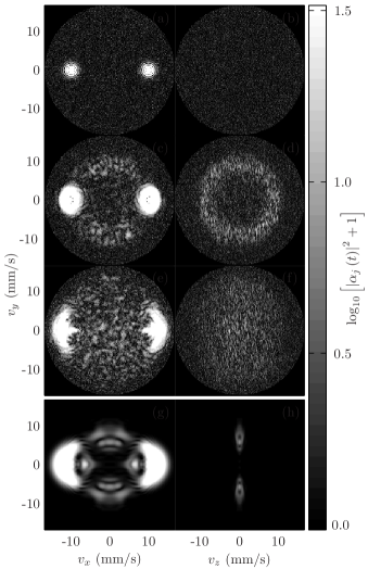
Figure 1: (a–f): Velocity mode populations on the planes $v_{z}=0$ (left) and $v_{x}=0$ (right) for the collision of packets generated from a six million atom condensate at $t=0$ (top), $t=0.5$ ms (middle) and $t=2.0$ ms (bottom). The spherical momentum cutoff is clearly visible in the upper plots due to the presence of quantum fluctuations. (g–h): Mode populations at $t=2.0$ ms for an identical collision excluding vacuum noise.

We consider collisions between two equally populated wavepackets derived from a single trapped condensate using a Bragg grating of very short duration compared to the overlap time of the packets Kozuma et al. (1999); Ovchinnikov et al. (1999). Thus an appropriate initial state, $\psi\left(\mathbf{x}\right)$ of the real particles is the sum of two distinct momentum wavepackets with the same spatial envelope:

$$\psi\left(\mathbf{x}\right)=\frac{1}{\sqrt{2}}\psi_{0}\left(\mathbf{x}\right)\left[e^{i\mathbf{k}_{+}\cdot\mathbf{x}}+e^{i\mathbf{k}_{-}\cdot\mathbf{x}}\right],$$ (5)

where $\psi_{0}\left(\mathbf{x}\right)$ is the stationary solution of the Gross-Pitaevskii equation for the $N_{0}$ atom condensate in a trap and $\mathbf{k}_{\pm}=\left(\pm mv_{c}/\hbar,0,0\right)$ are the wavepackets’ normalized amplitudes and wavevectors. For this paper we choose the case of a ${}^{23}\mathrm{Na}$ condensate in an axially symmetric trap with $\omega_{r}=2\pi\times 80$ Hz and $\omega_{z}=2\pi\times 20$ Hz, as used in Vogels et al. (2002), but with a maximum of $6\times 10^{6}$ atoms, compared to the maximum number $3\times 10^{7}$ used in the experiment. Immediately following the application of the Bragg pulses ($t=0$) the confining potential is removed, so that the evolution takes place in free space.

The velocity space population distribution for the collision of packets from an initial condensate of $6\times 10^{6}$ atoms with $v_{c}=10$ mm/s is shown in Fig. 1(a-f) for a sequence of times. This figure shows:

i) The original wavepackets broadening and changing shape from circular in projection to crescent shaped.

ii) The generation of a circular feature—the scattering halo—centered at the system center of mass velocity with a radius in velocity space approximately equal to (but larger than) $v_{c}$.

The scattering halo is characterized by patches of high mode population, the phase grains, whose size and aspect ratio are very similar to those of the original condensate packets (in velocity space). This characteristic size can be understood in terms of the parametric amplification of vacuum fluctuations described by Eq.(4). Pairs of vacuum modes $j$ and $r$ at each end of a diameter of the energy conservation sphere are selected preferentially for growth (or loss) if their phases are appropriate. The sum in Eq.(4) convolves the noise field near mode $r$ with the initial condensate packets, and if mode $r$ grows preferentially, it drives the growth of all modes near $j$ within a volume of the size of the condensate velocity wavefunction.

In the weakly populated regions separating the phase grains, analysis of our data reveals a large number of vortices, which is indicative of a turbulent velocity field and arises directly from the parametric amplification of the vacuum fluctuations. This justifies our identification of the behaviour as quantum turbulence. (An analogous amplification of electromagnetic vacuum fluctuations was achieved in 1982 using a Josephson junction Koch et al. (1982).)

In contrast, a simulation performed without the vacuum fluctuations generates a simple modulational instability, as shown in Fig. 1(g–h). The fluctuations are equivalent to $3\times 10^{6}$ additional particles, and thus their inclusion represents a significantly altered initial condition from that given by omitting them altogether.

As the halo generation process is analogous to parametric amplification, it is expected that modes of opposite velocity in the halo will display correlations, and that modes of similar velocity will similarly display correlations due to the finite size of the phase grains. Calculating these correlation functions should properly be performed on an ensemble of simulations. However, for this situation which, away from the condensate packets, displays a high degree of spherical homogeneity in velocity space, we can use a single simulation and average over modes in velocity space which have similar speeds and which are not occupied by the condensate packets. To this end we define the data collection region, consisting of those modes whose polar angles, $\varphi_{j}$, lie between $\pi/4$ and $3\pi/4$ to the positive $v_{x}$ axis. Clearly such a region would also be needed experimentally. Within this region then, we define the correlation functions

$$\!\!\!\!\bar{\mathcal{N}}\left(v,0\right) = \left\langle\left|\alpha_{j}\right|^{2}\right\rangle_{\left|{\bf v}\right|=v}-\frac{1}{2},$$ (6)

$$\!\!\!\!\bar{\mathcal{N}}\left(v,\delta{\bf v}\right) = {\rm Re}\left[\left\langle\alpha\left({\bf v}\right)^{*}\alpha\left({\bf v}+\delta{\bf v}\right)\right\rangle_{\left|{\bf v}\right|=v}\right]-\frac{\delta_{\delta{\bf v},0}}{2},$$ (7)

$$\!\!\!\!\bar{\mathcal{M}}\left(v\right) = \left\langle\alpha_{i}\alpha_{j}\right\rangle_{\left|{\bf v}\right|=v},$$ (8)

as the average non-condensate mode population (excluding virtual particles), the amplitude autocorrelation function and the pair creation correlation function respectively. The correlation functions for the six million atom simulation are shown through time in Fig. 2.

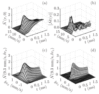
Figure 2: Correlation functions for the six million atom simulation averaged over the data collection region as described in the text: (a) average mode population; (b) pair creation correlation; (c,d) amplitude autocorrelation.

From Fig. 2(a), we observe that population builds up initially near $v=10$ mm/s, peaking at $t=0.52$ ms for $v=9.3$ mm/s. The subsequent redistribution of population within the halo modes occurs via inter-halo scattering events and can be considered as a thermalisation process.

Fig. 2(b) shows the pair creation correlation for the paired modes, $\mathbf{v}_{i}=-\mathbf{v}_{j}$ and shows that a definite, although small ($\approx 10$%), correlation develops, peaking at $t=0.30$ ms and then decaying as further scattering events occur.

Fig. 2(c,d) show the velocity space amplitude autocorrelation functions at $v=9.3$ mm/s. Fitting a Gaussian in $\delta v_{x,y,z}$ to obtain the FWHM correlation lengths, we find that from the time that population is established (at about $t=0.05$ ms) the ratio of the $\delta v_{x}$ and $\delta v_{y}$ correlation lengths to the $\delta v_{z}$ length remain close to 4. The individual lengths initially grow and peak at $t=0.25$ ms (where they are 1.2 mm/s in the $\delta v_{x}$ and $\delta v_{y}$ directions, and 0.3 mm/s in the $\delta v_{z}$ direction) and then decay slowly. These can be compared to the FWHM of the original velocity space condensate wavefunction, which is 0.7 mm/s in the $v_{x}$ and $v_{y}$ directions and 0.18 mm/s in the $v_{z}$ direction. This correlation behavior is a quantitative measure of the size of the phase grains, and we estimate the average number of atoms in a coherent patch to be 150 at $t=0.25$ ms for $v=9.3$ mm/s.

In Fig. 3 we examine the time evolution of the real particle population in the data collection region, defined using

$$N_{\rm dc}=\sum_{j}\left(\left|\alpha_{j}\right|^{2}-\frac{1}{2}\right),\hskip 14.22636pt\frac{\pi}{4}\leq\varphi_{j}\leq\frac{3\pi}{4},$$ (9)

for varying initial condensate number. For larger condensate numbers a larger fraction is scattered, and the scattering is completed earlier. The decrease in population at later times is due to interhalo scattering events redistributing population outside the data collection region.

For comparison, we plot the fraction of condensate population lost into the data collection region (assuming isotropic loss) during an identical collision using the complex scattering length method of Band et al. (2000). The most significant difference using our method is a considerably larger out-scattered fraction, because Bosonic stimulation is included. Additionally, the scattering model of Band et al. (2000) is essentially based on Fermi’s “golden rule”, which results in exact kinetic energy conservation at all times, and gives an initial linear growth of the out-scattered fraction. However, our method shows an initial quadratic growth rate, because the timescale over which one must average to derive the kinetic energy conservation implicit in the golden rule (say to an accuracy of about 10%) in this case is about $0.5{\rm s}$. As a result of both of these effects, the rate of population loss, instead of being greatest at $t=0$, where the wavepackets are maximally overlapped, is greatest at about $t=0.3$ – $0.5{\rm ms}$.

The major loss mechanism in a BEC is that of three body recombination Fedichev et al. (1996); Stamper-Kurn et al. (1998), but this can have very little effect on the results. Using the experimentally obtained loss rate, we estimate that in the time taken ($\approx 2{\rm ms}$) for an experiment, no more than 5 atoms would be lost from the system. Implementing a phenomenological three-body loss into our simulations shows no change in the dynamics until we increase the loss rate to more than 100 times the experimentally obtained value.

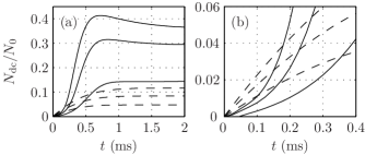
Figure 3: Normalised data collection region populations for the classical field simulations (sold lines) and complex scattering length simulations (dashed lines). Initial condensate numbers are (lowest to highest) $\left(1,3,6\right)\times 10^{6}$, all with $v_{c}=10$ mm/s. Subplot (b) shows the early times of (a).

Conclusions: This paper makes the first application of the classical field method to a realistic three dimensional problem, and produces results which could not have been generated by any other method in current use. Our detailed numerical results require only a single run of the simulation, avoiding time-consuming ensemble averages. Previous calculations Band et al. (2000); Vogels et al. (2002); Bach et al. (2002); Köhler and Burnett (2002) have been restricted to regimes in which Bosonic stimulation is not important, and have only been able to determine more limited information, whereas our method can handle very large ($\approx 40$%) outscattered fractions.

The only significant restriction on our method is the computer memory required to represent the system as it expands in space. For the situation considered here this is not a problem. Collisions with smaller out-scattered fractions would be more difficult to simulate because of the high ratio of virtual to real particle occupation, but the method would still be valid if sufficiently large ensembles of initial conditions were used, whereas for large out-scattered fractions, a single realization is sufficient for most measurable quantities.

New qualitative features found are: i) The existence of quantum turbulence, which should be easily detectable experimentally, using for example measurement of the density along a slice with the same techniques used to observe similar slices through clouds containing vortex lattices Raman et al. (2001); Haljan et al. (2001); ii) The suppression of the modulational instability which a simple Gross-Pitaevskii picture would predict; iii) The reduction in correlations expected between scattered atoms of opposite momentum to a rather small value.