Ultrafast electron dynamics in metals

Abstract

During the last decade, significant progress has been achieved in the rapidly growing field of the dynamics of hot carriers in metals. Here we present an overview of the recent achievements in the theoretical understanding of electron dynamics in metals, and focus on the theoretical description of the inelastic lifetime of excited hot electrons. We outline theoretical formulations of the hot-electron lifetime that is originated in the inelastic scattering of the excited quasiparticle with occupied states below the Fermi level of the solid. First-principles many-body calculations are reviewed. Related work and future directions are also addressed.

I Introduction

Recent advances in femtosecond laser technology have made possible the investigation of electron transfer processes at solid surfaces, which are known to be the basis for many fundamental steps in surface photochemistry and ultrafast chemical reactions.haight ; wolf ; nienhaus These are typically atomic and molecular adsorption processes and catalytic reactions between different chemical species, which transfer energy from the reaction complex into the nuclear and electronic degrees of freedom of the solid substrate. These reactions may induce elementary excitations, such as quantized lattice vibrations (phonons), collective electronic excitations (plasmons), and electron-hole (e-h) pairs. In metals, the excitation of e-h pairs leads to an excited or hot electron with energy above the Fermi level $\varepsilon_{F}$ and to an excited or hot hole with energy below $\varepsilon_{F}$. It is precisely the coupling of these hot carriers with the underlying substrate which governs the cross sections and branching ratios of electronically induced adsorbate reactions at metal surfaces.

It is the intent of this Review to discuss the current status of the rapidly growing field of the dynamics of hot carriers in metals. The energy relaxation of these hot electrons and holes is almost exclusively attributed to the inelastic scattering with cold electrons below the Fermi level (e-e scattering) and with phonons (e-ph scattering), since radiative recombination of e-h pairs may be neglected. Assuming that the excess energy of the hot carrier is much larger than the thermal energy $k_{B}T$, the e-e scattering rate does not depend on temperature. Furthermore, for excitation energies larger than $\sim 1\,{\rm eV}$ inelastic lifetimes are dominated by e-e scattering, e-ph interactions being in general of minor importance. Only at energies closer to the Fermi level, where the e-e inelastic lifetime increases rapidly, does e-ph scattering become important.phonons ; asier

Different techniques have recently become available for measuring hot-carrier lifetimes. Inverse photoemission (IPE)ipe and high resolution angle resolved photoemission (ARPE)matzdorf provide an indirect access to the lifetime of hot electrons and holes, respectively, by measuring the energetic broadening of transition lines after impigning an electron (IPE) or a photon (ARPE) into the solid. An alternative to IPE is two-photon photoemission (2PPE),fauster in which a first (pump) photon excites an electron from below the Fermi level to an intermediate state in the energy region $\varepsilon_{F}<\varepsilon<\varepsilon_{\rm vac}$ from where a second (probe) photon brings the electron to the final state above the vacuum level $\varepsilon_{\rm vac}$. This technique can also be used to acces the lifetime of the intermediate state directly in the time domain (time-resolved 2PPE),petek by measuring the decrease of the signal as the probe pulse is delayed with respect to the pump pulse. Recently, it has been demonstrated that lifetime measurements of electrons and holes in metals can be done by exploiting the capabilities of scanning tunneling microscopy (STM) and spectroscopy (STS),stm1 ; stm2 ; stm3 and ballistic electron emission spectroscopy (BEES) has also shown to be capable of determining hot-electron relaxation times in solid materials.bees ; claudia Applications of these techniques include not only measurements of the scattering rates of hot carriers in solids, but also measurements of the lifetime of Shockley and image-potential states at metal surfaces.review2

The early theoretical investigations of inelastic lifetimes and mean free paths of both low-energy electrons in bulk materials and image-potential states at metal surfaces have been described in previous reviews,rev1 ; rev2 showing that they strongly depend on the details of the electronic band structure.rev2 Nevertheless, although accurate measurements of inelastic lifetimes date back to the mid 1990’s, the first band-structure calculations of the e-e scattering in solids were not carried out until a few years ago.campillo1 ; ekardt ; campillo2 ; campillo3

Here we outline theoretical formulations of the hot-electron lifetime that is due to the inelastic scattering of the excited quasiparticle with occupied states below the Fermi level. Section 2 is devoted to the study of electron scattering processes in the framework of time-dependent perturbation theory. A discussion of the main factors that determine the decay of excited states is presented in Section 3, together with a review of the existing theoretical investigations of the lifetime of hot electrons in the bulk of a variety of metals. The inclusion of exchange-correlation effects and chemical potential renormalization is addressed in Section 4, and the final Section presents an overview and future directions.

Unless otherwise is stated, atomic units are used throughout, i.e., $e^{2}=\hbar=m_{e}=1$. Hence, we use the Bohr radius, $a_{0}=\hbar^{2}/m_{e}^{2}=0.529\AA$, as the unit of length and the Hartree, $H=e^{2}/a_{0}=27.2\,{\rm eV}$, as the unit of energy. The atomic unit of velocity is the Bohr velocity, $v_{0}=\alpha\,c=2.19\times 10^{8}\,{\rm cm\,s}^{-1}$, $\alpha$ and $c$ being the fine structure constant and the velocity of light, respectively.

II Theory

We take a Fermi system of $N$ interacting electrons at zero temperature ($T=0$), and consider an external excited electron interacting with the Fermi system. Fig. 1 depicts schematically a single inelastic scattering process for the excited hot electron. The hot electron in an initial state $\phi_{i}(\bf r)$ of energy $\varepsilon_{i}>\varepsilon_{F}$ is scattered into the state $\phi_{f}(\bf r)$ of energy $\varepsilon_{f}$ ($\varepsilon_{F}<\varepsilon_{f}<\varepsilon_{i}$) by exciting the cold Fermi system from its many-particle ground state of energy $E_{0}$ to some many-particle excited state of energy $E_{n}$ ($E_{n}-E_{0}=\varepsilon_{i}-\varepsilon_{f}$). By using the Fermi golden rule of time-dependent perturbation theory and keeping only the lowest-order term in the Coulomb interaction $v({\bf r},{\bf r}^{\prime})$ between the hot electron and the Fermi gas, the probability $P_{i\to f}$ per unit time for the occurrence of this process is found to bepitarke1

$$P_{i\to f} = -2\int d{\bf r}\int d{\bf r}^{\prime}\phi_{i}^{*}({\bf r})\,\phi_{f}^{*}({\bf r}^{\prime})\,$$ (1)

$$\times {\rm Im}W({\bf r},{\bf r}^{\prime},\varepsilon_{i}-\varepsilon_{f})\phi_{i}({\bf r}^{\prime})\,\phi_{f}({\bf r}),$$

where $W({\bf r},{\bf r}^{\prime},\omega)$ is the so-called screened interaction

$$W({\bf r},{\bf r}^{\prime};\omega) = v({\bf r},{\bf r}^{\prime})+\int d{\bf r}_{1}d{\bf r}_{2}v({\bf r},{\bf r}_{1})$$ (2)

$$\times \chi({\bf r}_{1},{\bf r}_{2};\omega)v({\bf r}_{2},{\bf r}^{\prime})$$

and $\chi({\bf r},{\bf r}^{\prime};\omega)$ is the density-response function of the interacting Fermi system.fetter

The total decay rate or reciprocal lifetime of the external excited electron in the initial state $\phi_{i}(\bf r)$ of energy $\varepsilon_{i}$ is simply the sum of the probabilities $P_{i\to f}$ over all available final states $\phi_{f}({\bf r})$ with energies $\varepsilon_{f}$, i.e.,

$$\tau_{i}^{-1}=\sum_{f}\,P_{i\to f},$$ (3)

where the final states are subject to the condition $\varepsilon_{F}<\varepsilon_{f}<\varepsilon_{i}$.

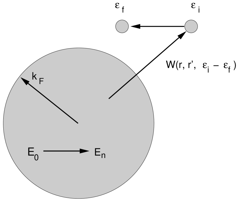
Figure 1: Scattering of an external excited electron with a Fermi system of $N$ interacting electrons at $T=0$. The external electron in an initial state of energy $\varepsilon_{i}>\varepsilon_{F}$ is scattered into an available state of energy $\varepsilon_{f}$ ($\varepsilon_{F}<\varepsilon_{f}<\varepsilon_{i}$) by exciting the cold Fermi system from its many-particle ground state of energy $E_{0}$ to some many-particle excited state of energy $E_{n}$ ($E_{n}-E_{0}=\varepsilon_{i}-\varepsilon_{f}$)

The single-particle wave functions and energies $\phi_{i,f}({\bf r})$ and $\varepsilon_{i,f}$ entering Eq. (1) can be chosen to be the eigenfuncions and eigenvalues of an effective Hartree,fetter Kohn-Sham,gross or quasiparticlegunnarsson ; nekovee hamiltonian.note2

II.1 Non-interacting Fermi sea

If the Fermi sea is assumed to be a system of non-interacting electrons moving in an effective potential, instead of Eqs. (1)-(2) one first considers the lowest-order probability $P_{i\to f}^{i^{\prime}\to f^{\prime}}$ per unit time for the excited hot electron in an initial state $\phi_{i}({\bf r})$ of enery $\varepsilon_{i}$ to be scattered into the state $\phi_{f}({\bf r})$ of energy $\varepsilon_{f}$ by exciting one single electron of the Fermi sea from an initial state $\phi_{i^{\prime}}({\bf r})$ of energy $\varepsilon_{i^{\prime}}$ to a final state $\phi_{f^{\prime}}({\bf r})$ of energy $\varepsilon_{f^{\prime}}$ (see Fig. 2), and then obtains the probability $P_{i\to f}$ by summing over all electrons in the Fermi sea (below the Fermi level) and all available final states for these electrons (above the Fermi level):

$$P_{i\to f}=4\pi\sum_{i^{\prime},f^{\prime}}n_{i^{\prime}}(1-n_{f^{\prime}})\left|v_{i,i^{\prime}}^{f,f^{\prime}}\right|^{2}\delta(\varepsilon_{i}-\varepsilon_{f}-\varepsilon_{f^{\prime}}+\varepsilon_{i^{\prime}}),$$ (4)

where

$$v_{i,i^{\prime}}^{f,f^{\prime}}=\int d{\bf r}\int d{\bf r}^{\prime}\phi_{i}^{*}({\bf r})\phi_{i^{\prime}}^{*}({\bf r}^{\prime})\,v({\bf r},{\bf r}^{\prime})\phi_{f}({\bf r})\phi_{f^{\prime}}({\bf r}^{\prime})$$ (5)

and $n_{i}$ are Fermi-Dirac occupation factors, which at $T=0$ are

$$n_{i}=\theta(\varepsilon_{F}-\varepsilon_{i}),$$ (6)

$\theta(x)$ being the Heaviside step function. The total decay rate $\tau_{i}^{-1}$ is obtained by summing over all available final states of the excited hot electron, as in Eq. (3).

Alternatively, on can simply replace the imaginary part of the interacting density-response function $\chi({\bf r},{\bf r}^{\prime};\omega)$ entering Eq. (2) by its non-interacting counterpart:

$${\rm Im}\,\chi^{0}({\bf r},{\bf r}^{\prime};\omega)=-2\pi\sum_{i^{\prime},f^{\prime}}n_{i^{\prime}}(1-n_{f^{\prime}})\phi_{i^{\prime}}^{*}({\bf r})\phi_{f^{\prime}}^{*}({\bf r}^{\prime})$$

$$\,\,\,\,\,\,\,\,\,\,\,\,\,\,\,\,\,\,\,\,\,\,\,\,\times\phi_{f^{\prime}}({\bf r})\phi_{i^{\prime}}({\bf r}^{\prime})\delta(\omega-\varepsilon_{f^{\prime}}+\varepsilon_{i^{\prime}}).$$ (7)

Introduction of Eq. (II.1) into Eqs. (1)-(2) yields again the probability of Eq. (4)

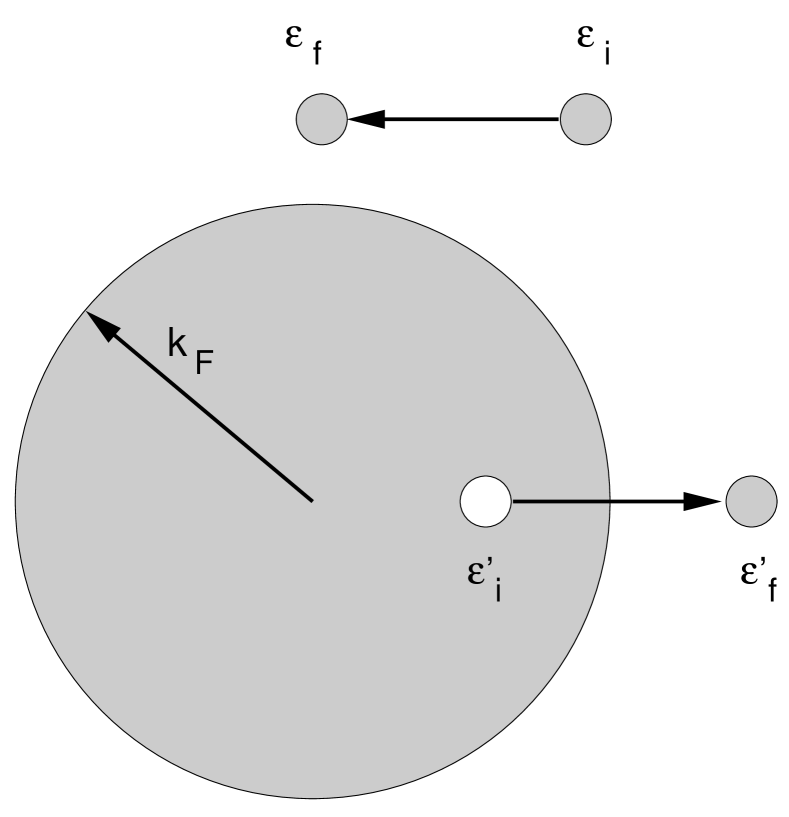
Figure 2: As in Fig. 1, but now the Fermi system is assumed to be a system of non-interacting electrons. Hence, single-electron scattering events are represented, where the external excited electron of energy $\varepsilon_{i}>\varepsilon_{F}$ is scattered into an available state of energy $\varepsilon_{f}$ ($\varepsilon_{F}<\varepsilon_{f}<\varepsilon_{i}$), as in Fig. 1, but now carrying one single electron of the Fermi sea from an initial state of energy $\varepsilon_{i^{\prime}}$ (below the Fermi level) to a final state of energy $\varepsilon_{f^{\prime}}$ (above the Fermi level).

Due to the long-range of the bare Coulomb interaction $v({\bf r},{\bf r}^{\prime})$ entering Eq. (5), this approach yields a total decay rate $\tau_{i}^{-1}$ that might be severely divergent, thereby resulting in a lifetime $\tau_{i}$ that would be equal to zero. However, many-body interactions of the Fermi sea, which are fully included in the interacting density-response function $\chi({\bf r},{\bf r}^{\prime};\omega)$ entering Eq. (2), are known to be responsible for a dynamical screening of the Coulomb interaction leading to a finite lifetime of excited hot electrons.

Many-body interactions of the Fermi sea are often approximately introduced by simply replacing the long-range bare Coulomb interaction $v({\bf r},{\bf r}^{\prime})$ entering Eq. (5) by the frequency-dependent screened interaction of Eq. (2) at the frequency $\omega=\varepsilon_{i}-\varepsilon_{f}$, although this does not yield in general a result equivalent to that of Eq. (1). In the long-wavelength limit, static ($\omega\to 0$) screening of the Fermi sea can be described by the Thomas-Fermi approximation,

$$W^{TF}({\bf r},{\bf r}^{\prime})=v({\bf r},{\bf r}^{\prime})\,{\rm e}^{-q_{TF}|{\bf r}-{\bf r}^{\prime}|}.$$ (8)

Here, $q_{TF}$ represents the Thomas-Fermi momentum, $q_{TF}=(4q_{F}/\pi)^{1/2}$, $q_{F}$ being the Fermi momentum.

II.2 Interacting Fermi sea: random-phase approximation (RPA)

In an interacting Fermi sea, we need to compute the full interacting density-response function $\chi({\bf r},{\bf r}^{\prime};\omega)$ entering Eq. (2). This function is also known to yield within linear-response theory the electron density induced in a many-electron system by an external potential $V^{ext}({\bf r},\omega)$:

$$\rho^{ind}({\bf r},\omega)=\int d{\bf r}^{\prime}\chi({\bf r},{\bf r}^{\prime};\omega)V^{ext}({\bf r}^{\prime},\omega).$$ (9)

For many years, the dynamical screening in an interacting Fermi system has been succesfully described in a time-dependent Hartree or, equivalently, random-phase approximation (RPA).fetter In this approach, the electron density induced by an external potential is obtained as the electron density induced in a non-interacting Fermi system by both the external potential $V^{ext}({\bf r},\omega)$ and the potential $V^{ind}({\bf r},\omega)$ induced by the induced electron density itself

$$V^{ind}({\bf r},\omega)=\int d{\bf r^{\prime}}v({\bf r},{\bf r}^{\prime})\rho^{ind}({\bf r}^{\prime},\omega).$$ (10)

Hence, in this approximation

$$\rho^{ind}({\bf r},\omega)=\int d{\bf r}^{\prime}\left[\chi^{0}({\bf r},{\bf r}^{\prime};\omega)+\int d{\bf r}_{1}\right.$$

$$\left.\times\int d{\bf r}_{2}\chi^{0}({\bf r},{\bf r}_{1};\omega)v({\bf r}_{1},{\bf r}_{2})\chi({\bf r}_{2},{\bf r}^{\prime};\omega)\right]V^{ext}({\bf r}^{\prime},\omega),$$

where $\chi^{0}({\bf r},{\bf r}^{\prime};\omega)$ is the density-response function of a system of non-interacting electrons. Comparing Eqs. (9) and (II.2), one finds that in the RPA the interacting density-response function is obtained from the knowledge of the non-interacting density-response function by solving the integral equation

$$\chi({\bf r},{\bf r}^{\prime};\omega) = \chi^{0}({\bf r},{\bf r}^{\prime};\omega)+\int d{\bf r}_{1}\int d{\bf r}_{2}\,\chi^{0}({\bf r},{\bf r}_{1};\omega)$$ (12)

$$\times v({\bf r}_{1},{\bf r}_{2})\,\chi({\bf r}_{2},{\bf r}^{\prime};\omega).$$

III Results

III.1 General considerations

The decay rate of excited electrons in an interacting Fermi sea is obtained from Eqs. (1)-(3), the main ingredients being the hot-electron initial and final states [$\phi_{i}({\bf r})$ and $\phi_{f}({\bf r})$] and the imaginary part of the screened interaction $W({\bf r},{\bf r}^{\prime};\omega)$. ${\rm Im}W({\bf r},{\bf r}^{\prime};\omega)$ contains both a measure of the probability for creating single-particle and collective excitations in a many-electron system and a measure of the screening of the interaction between the hot electron and the Fermi sea. In the case of low energies, where collective modes cannot be produced, the hot-electron lifetime is mainly determined by a competition between (i) the coupling of the initial state $\phi_{i}({\bf r})$ with available states $\phi_{f}({\bf r})$ above the Fermi level, (ii) the phase space available for the creation of electron-hole (e-h) pairs, and (iii) the dynamical screening of the Fermi sea.

III.1.1 Coupling with available states above the Fermi level

The coupling of the excited electron $\phi_{i}({\bf r})$ with available states $\phi_{f}({\bf r})$ above the Fermi level strongly depends on whether the excited quasiparticle is a bulk or a surface state.

A partially occupied band of Shockley surface states typically occurs in the gap of free-electron-like $s$,$p$ bands.shoc1 ; shoc2 ; shoc3 Another class of surface states occurs in the vacuum region of metal surfaces with a band gap near the vacuum level. These are unoccupied Rydberg-like image-potential states, which appear as a result of the self-interaction that an electron near the surface suffers from the polarization charge it induces at the surface.echenique ; smith

Fig. 3 shows schematically the projection of the bulk band structure onto the (111) surface of the noble metal Cu. At the $\bar{\Gamma}$ point ($k_{\parallel}=0$), the projected band gap extends from $0.9\,{\rm eV}$ below to $4.23\,{\rm eV}$ above the Fermi level, in such a way that both a Shockley ($n=0$) and an image ($n=1$) state are supported.

Shockley surface states are known to be localized near the topmost atomic layer. However, image states are mainly localized outside the solid. Therefore, image states are expected to be weakly coupled with available bulk states above the Fermi level and to live much longer than excited bulk states with the same energy: while the RPA broadening (or linewidth) $\tau_{i}^{-1}$ of a bulk state at the energy of the $n=1$ image state on Cu(111) ($\varepsilon_{i}-\varepsilon_{F}=4.12\,{\rm eV}$) is found to be $304\,{\rm meV}$, the $n=1$ image-state linewidth is reduced to $29\,{\rm eV}$.imanol2

Coupling of the image state with the crystal occurs through the decay into bulk unoccupied states lying below the bottom of the projected band gap (which yields a linewidth of $17\,{\rm meV}$) and also through the decay into the unoccupied part of the $n=0$ Shockley surface state lying within the projected band gap (which leads to a linewidth of $12\,{\rm meV}$). A measure of the coupling of image states to bulk states of the solid can be given approximately by the penetration of the image-state wave function into the solid, which in the case of the $n=1$ image state on Cu(111) is found to be of $22\%$. However, the contribution to the linewidth coming from the decay into bulk states ($17\,{\rm meV}$) is still well below $0.22$ times the linewidth of a bulk state at the energy of the image state, i.e., $0.22\times 304\,{\rm meV}$). This is due to the presence of a projected band gap at the surface, which in the case of Cu(111) reduces considerably the phase space available for real transitions of the $n=1$ image state into bulk unoccupied states. This considerable reduction of the available phase space for real transitions does not occur in the case of Cu(100); this explains the known fact that although the penetration of the $n=1$ image state on Cu(100) is approximately 4 times smaller than in the case of Cu(111) the ratio between the linewidths of the $n=1$ image state on the (111) and (100) surfaces of Cu is smaller than 2.imanol2

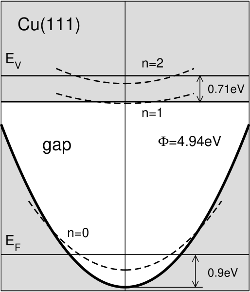
Figure 3: Schematic representation of the electronic band structure of the (111) surface of Cu.

III.1.2 Phase space versus dynamical screening

In the case of simple metals that can be described by a uniform free-electron gas of density $n_{0}$, which is characterized by the density parameter $r_{s}=(3/4\pi n_{0})^{1/3}/a_{0}$, a careful analysis of the phase space available for the creation of e-h pairs yields a decay rate of hot electrons with energies near the Fermi level ($\varepsilon_{i}-\varepsilon_{F}<<\varepsilon_{i}$) of the formrev2

$$\tau_{i}^{-1}=f(r_{s})(\varepsilon_{i}-\varepsilon_{F})^{2}.$$ (13)

Furthermore, in the high-density limit ($r_{s}\to 0$), Eqs. (1)-(3) yieldrev2 ; qf ; note3

$$f(r_{s})={(3\pi^{2}/2)^{1/3}\over 36}\,r_{s}^{5/2}.$$ (14)

This simple formula shows that the decay rate decreases as the electron density increases, which is also found to be true in the case of simple and noble metals ($2<r_{s}<6$) and hot electrons with energies lying a few electronvolts above the Fermi level.

As the electron density increases, the density of states (DOS) is known to increase. Hence, one might be tempted to conclude that as the electron density increases there are more electrons available for the creation of e-h pairs near the Fermi level, which would eventually yield an enhanced hot-electron decay. However, Eq. (14) shows that this is not the case. The reason for this behaviour is twofold. On the one hand, due to momentum and energy conservation the number of states available for real transitions in metals is typically weakly dependent on the actual electron density. On the other hand, as the electron density increases the ability of electrons to screen the Coulomb interaction with the external excited electron also increases, which leads to a smaller screened interaction and a reduced hot-electron decay.

Fig. 4 shows the DOS of a free-electron gas with the electron density $n_{0}$ equal to the average density of valence electrons in the simple metals Al ($r_{s}=2.07$) and Na ($r_{s}=3.99$), together with the corresponding RPA linewidths [as obtained from Eqs. (1)-(3)] of hot electrons with energy lying $1\,{\rm eV}$ above the Fermi level. While in the case of Al, with a large DOS near the Fermi level, the linewidth is $14\,{\rm meV}$, the linewidth of hot electrons with $\varepsilon_{i}-\varepsilon_{F}=1\,{\rm eV}$ in Na is $59\,{\rm meV}$. Hence, hot electrons live longer in Al than in Na, which is basically due to the strong screening characteristic of high-density metals like Al.

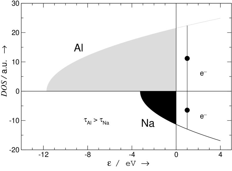
Figure 4: Density of states of a free-electron gas with the electron density $n_{0}$ equal to the average density of valence electrons in Al ($r_{s}=2.07$) and Na ($r_{s}=3.99$). The RPA linewidth of high-density Al is found to be considerably smaller than the corresponding linewidth of low-density Na.

III.2 Free-electron gas

For many years, theoretical predictions of the electron dynamics of bulk states in solids had been based on a free-electron gas (FEG) or jellium description of the solid, in which a homogeneous assembly of interacting electrons is assumed to be immersed in a uniform positive background. In this model there is translational invariance, the one-particle states entering Eq. (1) are momentum eigenfunctions, and Eqs. (1)-(3) are easily found to yield

$$\tau_{\bf k}^{-1}=-2\int{d{\bf q}\over(2\pi)^{3}}\,{\rm Im}W_{{\bf q},\omega},$$ (15)

where the energy transfer $\omega=\varepsilon_{\bf k}-\varepsilon_{{\bf k}-{\bf q}}$ [here, $\varepsilon_{\bf k}=k^{2}/2$] is subject to the condition $0<\omega<\varepsilon_{\bf k}-\varepsilon_{F}$, and

$$W_{{\bf q},\omega}=v_{\bf q}+v_{\bf q}\,\chi_{{\bf q},\omega}\,v_{\bf q},$$ (16)

$v_{\bf q}$ and $\chi_{{\bf q},\omega}$ being Fourier transforms of the bare Coulomb interaction $v({\bf r},{\bf r}^{\prime})$ and the interacting density-response function $\chi({\bf r},{\bf r}^{\prime};\omega)$, respectively. The screened interaction $W_{{\bf q},\omega}$ is usually expressed in terms of the inverse dielectric function $\epsilon_{{\bf q},\omega}^{-1}$, as follows

$$W_{{\bf q},\omega}=v_{\bf q}\,\epsilon_{{\bf q},\omega}^{-1},$$ (17)

where

$$\epsilon_{{\bf q},\omega}^{-1}=1+\chi_{{\bf q},\omega}\,v_{\bf q}.$$ (18)

III.2.1 Non-interacting Fermi sea

If the Fermi sea is assumed to be a system of non-interacting electrons, $\chi_{{\bf q},\omega}$ reduces to the well-known Lindhard function $\chi_{{\bf q},\omega}^{0}$,pines ; lindhard . One can then write the imaginary part of the screened interaction of Eq. (16) as

$${\rm Im}W_{{\bf q},\omega}^{0} = -2\pi\int{d{\bf k}^{\prime}\over(2\pi)^{3}}n_{{\bf k}^{\prime}}(1-n_{{\bf k}^{\prime}+{\bf q}})$$ (19)

$$\times \left|v_{\bf q}\right|^{2}\delta(\omega-\omega_{{\bf k}^{\prime}+{\bf q}}+\omega_{{\bf k}^{\prime}}).$$

III.2.2 Interacting Fermi sea: RPA

In the RPA, the interacting density-response function $\chi_{{\bf q},\omega}^{0}$ is obtained from Eq. (12), i.e.,

$$\chi_{{\bf q},\omega}=\chi^{0}_{{\bf q},\omega}+\chi_{{\bf q},\omega}^{0}\,v_{\bf q}\,\chi_{{\bf q},\omega},$$ (20)

or, equivalently [see Eq. (18)],

$$\epsilon_{{\bf q},\omega}=1-\chi^{0}_{{\bf q},\omega}\,v_{\bf q}.$$ (21)

Introducing Eq. (20) into Eq. (16), one finds

$${\rm Im}W_{{\bf q},\omega} = -2\pi\int{d{\bf k}^{\prime}\over(2\pi)^{3}}n_{{\bf k}^{\prime}}(1-n_{{\bf k}^{\prime}+{\bf q}})$$ (22)

$$\times \left|W_{{\bf q},\omega}\right|^{2}\delta(\omega-\omega_{{\bf k}^{\prime}+{\bf q}}+\omega_{{\bf k}^{\prime}}),$$

which is of the form of Eq. (19) with the bare Coulomb interaction $v_{\bf q}$ replaced by the RPA screened interaction $W_{{\bf q},\omega}$. Beyond the RPA, ${\rm Im}W_{{\bf q},\omega}$ cannot always be expressed as in Eq. (22).

We note that in the high-density limit ($r_{s}\to 0$) and for hot electrons with energies lying near the Fermi level ($\varepsilon_{\bf k}-\varepsilon_{F}<<\varepsilon_{\bf k}$), introduction of Eq. (22) into Eq. (15) yields the decay rate given by Eqs. (13) and (14), which will be referred as $\tau_{QF}^{-1}$.

Figs.  6 and 7 show the RPA lifetime $\tau_{\bf k}$ of hot electrons in a free-electron gas, divided by $\tau_{QF}$, as a function of the electron-density parameter $r_{s}$ for hot electrons in the vicinity of the Fermi surface (Fig. 5), and as a function of $\varepsilon_{\bf k}-\varepsilon_{F}$ for an electron density equal to that of valence electrons in Al (Fig. 6). Although the high-density limit of Eq. (14) only reproduces the full RPA calculation as $r_{s}\to 0$, Fig. 5 shows that differences between this high-density approximation ($\tau_{QF}$) and the full RPA calculation ($\tau$) are very small at electron densities with $r_{s}<2$ and go up to no more than $7\%$ at $r_{s}=6$. In the inset of Fig. 5 the RPA lifetime is represented, showing that as occurs in the high-density limit [see Eq. (14)] the RPA lifetime $\tau_{\bf k}$ increases very rapidly with the electron density.

In the limit $\varepsilon_{\bf k}\to\varepsilon_{F}$ the available phase space for real transitions is simply $\varepsilon_{\bf k}-\varepsilon_{F}$, which yields the $(\varepsilon_{\bf k}-\varepsilon_{F})^{2}$ quadratic scaling of Eq. (13). However, as the energy increases momentum and energy conservation prevents the available phase space from being as large as $\varepsilon_{\bf k}-\varepsilon_{F}$. As a result, the actual lifetime departures from the quadratic scaling predicted for electrons in the vicinity of the Fermi level (see Fig. 6), differences between the full RPA lifetime $\tau_{\bf k}$ and the lifetime $\tau_{QF}$ dictated by Eqs. (13) and (14) ranging from $\approx 0.5\%$ at $\varepsilon_{\bf k}\approx\varepsilon_{F}$ to $\approx 40\%$ at $\varepsilon_{\bf k}-\varepsilon_{F}=4\,{\rm eV}$.

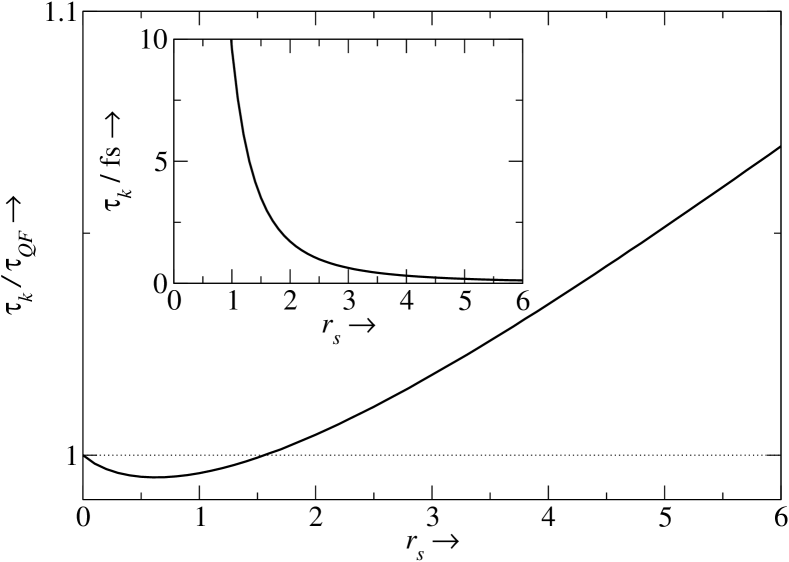
Figure 5: RPA lifetime $\tau_{k}$ of hot electrons in a free-electron gas, divided by $\tau_{QF}$ [Eqs. (13) and (14)], as a function of the electron-density parameter $r_{s}$ and for hot electrons in the vicinity of the Fermi surface.

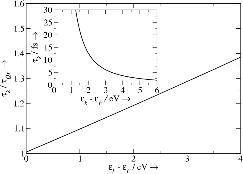
Figure 6: RPA lifetime $\tau_{k}$ of hot electrons in a free-electron gas, divided by $\tau_{QF}$ [Eqs. (13) and (14)], as a function of $\varepsilon_{k}-\varepsilon_{F}$ for an electron density equal to that of valence electrons in Al ($r_{s}=2.07$)

III.3 Random-$k$ approximation

For the description of lifetimes and inverse mean free paths (IMFP) in non-free-electron solids, several authors have employed the so-called random-$k$ approximation first considered by Berglund and Spicerberglund and by Kane.kane The starting point of this approximation is Eq. (4) with the bare Coulomb interaction $v({\bf r},{\bf r}^{\prime})$ replaced by a frequency-dependent screened interaction $W({\bf r},{\bf r}^{\prime};\omega)$. The random-$k$ approximation is then the result of replacing all the squared matrix elements $\left|W_{i\to f}^{i^{\prime}\to f^{\prime}}(\omega)\right|^{2}$ by their average $M_{i}$ over all available states $i^{\prime}$, $f^{\prime}$, and $f$. All the summations entering Eqs. (3) and (4) can then be replaced by integrations over the corresponding density of states, and one can write the reciprocal lifetime as

$$\tau_{i}^{-1}={\pi\over 2}\,M_{i}\,\int_{\varepsilon_{F}}^{\varepsilon_{i}}d\varepsilon\,\rho(\varepsilon)\int_{\varepsilon_{F}-(\varepsilon_{i}-\varepsilon)}^{\varepsilon_{F}}d\varepsilon^{\prime}\,\rho(\varepsilon^{\prime})\rho(\varepsilon_{i}+\varepsilon^{\prime}-\varepsilon),$$ (23)

where the quantities $\rho(\varepsilon)$ are assumed to include spin, i.e.,

$$\int_{-\infty}^{+\infty}d\varepsilon\rho(\varepsilon)=N,$$ (24)

$N$ being the total number of electrons.

A further simplification may be achieved if the density of states is assumed to take the constant value $\rho_{i}$ below and above the Fermi level. Eq. (23) then reduces to

$$\tau_{i}^{-1}={\pi\over 4}\,\rho_{i}^{3}\,M_{i}^{2}\,(\varepsilon_{i}-\varepsilon_{F})^{2}.$$ (25)

As the electron density increases, both the DOS and the screening of the Fermi sea increase. Since an enhanced screening yields a reduced $M_{i}$ factor, the actual dependence of the hot-electron lifetime on the electron density would be the result of the competition between DOS and screening effects. Screening effects typically dominate leading to a lifetime that increases with the electron density, as occurs in the case of a free-electron gas.

The random-$k$ approximation was first used by Berglund and Spicer in order to explain experimental photoemission studies of Cu and Ag.berglund Scattering rates of electrons in Si were computed by Kane,kane and Krolikowsky and Spicerks employed the random-$k$ approximation to calculate the energy dependence of the IMFP of electrons in Cu from the knowledge of density-of-state-distributions in this material which had been deduced from photoelectron energy-distribution measurements.

More recently, Penn et al. used the random-$k$ approximation to analyze the spin-polarized electron-energy-loss spectra and hot-electron lifetimes in ferromagnetic Fe, Ni, Co, and Fe-B-Si alloys.penn1 ; penn2 The experimental spin-dependent lifetime of the $n=1$ image state on Fe(110) was also interpreted by using this approximation.passek Drouhin developed a model to evaluate the scattering cross section and spin-dependent inelastic mean free path from the knowledge of density-of-state distributions, and applied it to Cr, Fe, Co, Ni, Gd, Ta, and the noble metals Cu, Ag, and Au.drouhin An analogous approach was developed by Zarate et al., where simple approximations to the DOS were used to obtain analytical expressions for the electron lifetimes in transition metals.zarate

The random-$k$ approximation has also been discussed and compared to first-principles calculations by Zhukov et al..zhukov11 ; zhukov2 It was shown that when initial and final states are either both $sp$ or both $d$ states then with a proper choice of the averaged matrix elements $M_{i}$ Eq. (23) yields lifetimes in reasonable agreement with more elaborated calculations.

III.4 First-principles calculations

First-principles calculations of the scattering rates of hot-electrons in periodic solids were first carried out only a few years ago by Campillo et al..campillo1 In this work, hot-electron inverse lifetimes were obtained from the knowledge of the on-shell electron self-energy of many-body theory, which in the so-called $G^{0}W$ approximation yields exactly the same result as Eqs. (1)-(3) above.

For periodic crystals, the single-particle wave functions entering Eq. (1) are Bloch states $\phi_{{\bf k},i}({\bf r})$ and $\phi_{{\bf k}-{\bf q},f}({\bf r})$ with energies $\varepsilon_{{\bf k},i}$ and $\varepsilon_{{\bf k}-{\bf q},f}$, $i$ and $f$ representing band indices. Hence, introducing Eq. (1) into Eq. (3) and Fourier transforming one finds

$$\tau_{{\bf k},i}^{-1}= - 2\sum_{f}\int{d{\bf q}\over(2\pi)^{3}}\sum_{{\bf G},{\bf G}^{\prime}}B_{i,f}^{*}({\bf q}+{\bf G})$$ (26)

$$\times B_{i,f}({\bf q}+{\bf G}^{\prime})\,{\rm Im}W_{{\bf G},{\bf G}^{\prime}}({\bf q},\omega),$$

where the energy transfer $\omega=\varepsilon_{{\bf k},i}-\varepsilon_{{\bf k}-{\bf q},f}$ is subject to the condition $0<\omega<\varepsilon_{{\bf k},i}-\varepsilon_{F}$, the integration is extended over the first Brillouin zone (BZ), the vectors ${\bf G}$ and ${\bf G}^{\prime}$ are reciprocal lattice vectors, $B_{if}$ represent matrix elements of the form

$$B_{i,f}({\bf q}+{\bf G})=\int d{\bf r}\phi_{{\bf k},i}^{*}({\bf r})\,{\rm e}^{i({\bf q}+{\bf G})\cdot{\bf r}}\phi_{{\bf k}-{\bf q},f}({\bf r}),$$ (27)

and $W_{{\bf G},{\bf G}^{\prime}}({\bf q},\omega)$ are Fourier coefficients of the screened interaction $W({\bf r},{\bf r}^{\prime};\omega)$. As in the case of the free-electron gas, the Fourier coefficients $W_{{\bf G},{\bf G}^{\prime}}({\bf q},\omega)$ are usually expressed in terms of the inverse dielectric matrix

$$W_{{\bf G},{\bf G}^{\prime}}({\bf q},\omega)=v({\bf q}+{\bf G})\,\epsilon_{{\bf G},{\bf G}^{\prime}}^{-1}({\bf q},\omega),$$ (28)

$v(\bf q)$ being the Fourier transform of the bare Coulomb interaction $v({\bf r},{\bf r}^{\prime})$. In the RPA,

$$\epsilon_{{\bf G},{\bf G}^{\prime}}({\bf q},\omega)=\delta_{{\bf G},{\bf G}^{\prime}}-\chi_{{\bf G},{\bf G}^{\prime}}^{0}({\bf q},\omega)\,v({\bf q}+{\bf G}^{\prime}),$$ (29)

where $\chi_{{\bf G},{\bf G}^{\prime}}^{0}({\bf q},\omega)$ are Fourier coefficients of the non-interacting density-response function $\chi^{0}({\bf r},{\bf r}^{\prime};\omega)$.

Couplings of the wave vector ${\bf q}+{\bf G}$ to wave vectors ${\bf q}+{\bf G}^{\prime}$ with ${\bf G}\neq{\bf G}^{\prime}$ appear as a consequence of the existence of electron-density variations in the solid. If these terms, representing the so-called crystalline local-field effects, are neglected, one can write Eq. (26) as

$$\tau_{{\bf k},i}^{-1}=2\sum_{f}{{}^{\prime}}\int{d{\bf q}\over(2\pi)^{3}}\sum_{{\bf G},{\bf G}^{\prime}}B_{i,f}^{*}({\bf q}+{\bf G})$$ (30)

$$\times B_{i,f}({\bf q}+{\bf G})\,v({\bf q}+{\bf G}){{\rm Im}\,\epsilon_{{\bf G},{\bf G}}({\bf q},\omega)\over\left|\epsilon_{{\bf G},{\bf G}}({\bf q},\omega)\right|^{2}}.$$

This expression accounts explicitly for the three main ingredients entering the hot-electron decay process. First of all, the coupling of the hot electron with available states above the Fermi level is dictated by the matrix elements $B_{i,f}({\bf q}+{\bf G})$. Secondly, the imaginary part of the dielectric matrix $\epsilon_{{\bf G},{\bf G}}({\bf q},\omega)$ represents a measure of the number of states available for the creation of e-h pairs with momentum and energy ${\bf q}+{\bf G}$ and $\omega$, respectively. Thirdly, the dielectric matrix in the denominator accounts for the many-body e-e interactions in the Fermi sea, which dynamically screen the interaction with the external hot electron.

Since for a given hot-electron energy $\varepsilon$ there are in general various possible wave vectors and bands, one can define an energy-dependent reciprocal lifetime by doing an average over wave vectors and bands. As a result of the symmetry of Bloch states, one finds $\tau^{-1}_{S{\bf k},i}=\tau^{-1}_{{\bf k},i}$, with $S$ representing a point group symmetry operation in the periodic crystal. Thus, one can write

$$\tau^{-1}(\varepsilon)=\frac{\sum_{n}\sum_{\bf k}^{\rm IBZ}\,m_{{\bf k},n}\tau^{-1}_{{\bf k},n}}{\sum_{n}\sum_{\bf k}^{\rm IBZ}\,m_{{\bf k},n}},$$ (31)

where $m_{{\bf k},n}$ represents the number of wave vectors ${\bf k}$ lying in the irreducible element of the Brillouin zone (IBZ) with the same energy $\varepsilon$.

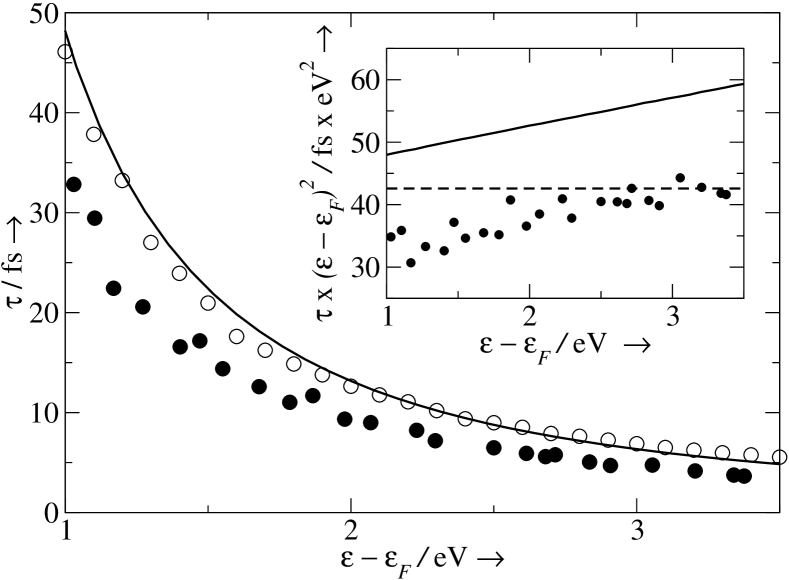
Figure 7: Hot-electron lifetimes in Al, as a function of the hot-electron energy $\varepsilon$ with respect to the Fermi level $\varepsilon_{F}$. Solid circles represent the ab initio RPA calculation, as obtained after averaging the lifetime broadening $\tau_{{\bf k},i}^{-1}$ of Eq. (26) over all states with the same energy $\varepsilon$. The solid line represents the RPA lifetime of hot electrons in a FEG with $r_{s}=2.07$. Open circles represent the result obtained from Eq. (26) by replacing the hot-electron initial and final states entering the coefficients $B_{if}$ by plane waves, but with full inclusion of the band structure in the evaluation of ${\rm Im}W_{{\bf G},{\bf G}^{\prime}}({\bf q},\omega)$. The inset exhibits scaled lifetimes of hot electrons in Al. Solid circles and the solid line represent first-principles and FEG calculations, respectively, both within RPA. The dashed line represents the prediction of Eqs. (13) and (14).

III.4.1 Plane-wave (PW) basis

The calculations reported in Refs. campillo1 ; campillo2 ; campillo3 for the lifetime of hot electrons in the simple metals Al, Mg, and Be, and the noble metals Cu and Au were carried out from Eqs. (26)-(29) by expanding all one-electron Bloch states in a plane-wave (PW) basis:

$$\phi_{{\bf k},i}({\bf r})={1\over\Omega}\,\sum_{\bf G}u_{{\bf k},i}({\bf G})\,{\rm e}^{{\rm i}\,({\bf k}+{\bf G})\cdot{\bf r}},$$ (32)

where $\Omega$ represents the normalization volume. More recently, similar calculations were reported by Bacelar et al. for the lifetime of hot electrons in six transition metals: two fcc metals (Rh and Pd), two bcc metals (Nb and Mo), and two hcp metals (Y and Ru).bacelar

In this approach, one first solves self-consistently for the coefficients $u_{{\bf k},i}({\bf G})$ the Kohn-Sham equation of density-functional theory (DFT), with use of the local-density approximation (LDA) for exchange and correlationperdew and non-local norm-conserving ionic pseudopotentialspseudo to describe the electron-ion interaction. From the knowledge of the eigenfunctions and eigenvalues of the Kohn-Sham hamiltonian, one can proceed to evaluate the non-interacting density-response matrix $\chi_{{\bf G},{\bf G}^{\prime}}^{0}({\bf q},\omega)$ (see, e.g., Ref. rev2 ) and the dielectric matrix $\epsilon_{{\bf G},{\bf G}^{\prime}}({\bf q},\omega)$, a matrix equation must then be solved for the inverse dielectric matrix, and the scattering rate is finally computed from Eq. (26) with full inclusion of crystalline local-field effects.

Here, we are showing the results of ab initio RPA calculations of the average lifetime of hot electrons in the simple metal Al and the noble metals Cu and Au, all obtained from Eqs. (26)-(29) and (31), and we compare these results to the RPA lifetime of hot electrons in the corresponding FEG as obtained from Eqs. (15) and (16). Both ab initio and FEG calculations were performed within the very same many-body framework, and the comparison between them indicates that while band-structure effects reduce the lifetime of hot electrons in Al, the presence of non-free-electron-like $d$ bands in the noble metals considerably enhances the lifetime of hot electrons in Cu and Au.

In Fig. 7, we show ab initio (solid circles) and FEG (solid line) RPA calculations of the average lifetime $\tau(\varepsilon)$ [see Eq. (31)] of hot electrons in the face-centered-cubic (fcc) Al, as a function of the hot-electron energy $\varepsilon$ with respect to the Fermi level $\varepsilon_{F}$.campillo1 These calculations show that even in a free-electron metal like Al band-structure effects play a key role lowering the hot-electron lifetime by a factor of $\sim 0.65$ for all electron energies under study. In order to understand the origin of band-structure effects, an additional calculation is represented by open circles where the hot-electron initial and final Bloch states entering the coefficients $B_{i,f}$ of Eq. (27) have been replaced by plane waves (as in a FEG) but keeping the full inverse dielectric matrix of the crystal. This calculation, which lies nearly on top of the FEG curve, shows that band-structure effects on both e-h pair creation and the dynamical screening of the Fermi sea are very small, as occurs in the case of slow ions.ions However, the coupling of hot-electron initial and final Bloch states appears to be very sensitive to the band structure, which in the case of Al shows a characteristic splitting over the Fermi level thereby opening new channels for electron decay and reducing the lifetime.campillo2

Similar results to those exhibited in Fig. 7 for Al were obtained for the hexagonal closed-packed (hcp) Mg,campillo2 whose band structure also splits just above the Fermi level along certain symmetry directions. However, the splitting of the band structure of this material is not as pronounced as in the case of Al, and the departure of the hot-electron lifetime in Mg from the corresponding FEG calculation with $r_{s}=2.66$ was found to be of about $25\%$, smaller than in Al.

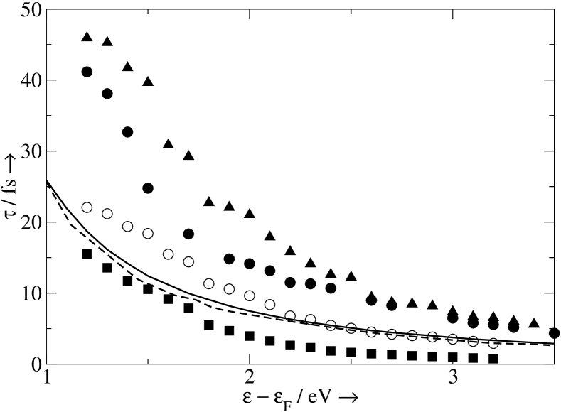
Figure 8: Hot-electron lifetimes in Cu, as a function of the hot-electron energy $\varepsilon$ with respect to the Fermi level $\varepsilon_{F}$. Solid circles represent the ab initio RPA calculation, as obtained after averaging the lifetime broadening $\tau_{{\bf k},i}^{-1}$ of Eq. (26) over all states with the same energy $\varepsilon$. The solid line represents the RPA lifetime of hot electrons in a FEG with $r_{s}=2.67$. The dotted line represents the ab initio RPA calculation of the average lifetime $\tau(\varepsilon)$, but with the $3d$ shell assigned to the core in the pseudopotential generation. The squares represent the result of replacing in Eq. (30) all one-electron Bloch states by plane waves (FEG calculation) but keeping the actual density of states in the evaluation of ${\rm Im}\epsilon_{{\bf G},{\bf G}^{\prime}}({\bf q},\omega)$. Open circles represent the result obtained from Eq. (30) by replacing the hot-electron initial and final states enetring the coefficients $B_{if}$ by plane waves and the dielectric function in $|\epsilon_{{\bf G},{\bf G}}({\bf q},\omega)|^{-2}$ by that of a FEG with $r_{s}=2.67$, but with full inclusion of the band structure in the calculation of ${\rm Im}\epsilon_{{\bf G},{\bf G}^{\prime}}({\bf q},\omega)$. Triangles represent the result obtained from Eq. (30) by replacing the hot-electron initial and final states entering the coefficients $B_{if}$ by plane waves, but with full inclusion of the band structure in the evaluation of both ${\rm Im}\epsilon_{{\bf G},{\bf G}^{\prime}}({\bf q},\omega)$ and $|\epsilon_{{\bf G},{\bf G}}({\bf q},\omega)|^{-2}$.

Figs. 8-10 exhibit ab initio (solid circles) and FEG (solid lines) RPA calculations of the average lifetime $\tau(\varepsilon)$ of hot electrons in the fcc metals Cu and Au, again as a function of the hot-electron energy $\varepsilon$ with respect to the Fermi level. Cu and Au are noble metals with entirely filled $3d$ and $5d$ bands, respectively. Slightly below the Fermi level, at $\varepsilon-\varepsilon_{F}\sim 2\,{\rm eV}$, we have $d$ bands capable of holding 10 electrons per atom, the one remaining electron being in both Cu and Au in a free-electron-like band below and above the $d$ bands. Hence, a combined description of both delocalized $s$ valence bands and localized $d$ bands is needed to address the actual electronic response of these metals. The results reported in Refs. campillo1 ; campillo2 ; campillo3 and presented in Figs. 8-10 where found by keeping all $4s^{1}$ and $3d^{10}$ Bloch states (in the case of Cu) and all $6s^{1}$ and $5d^{10}$ Bloch states (in the case of Au) as valence electrons in the generation of the pseudopotential.

Also represented in Fig. 8 are additional calculations for the hot-electron lifetime in Cu, which help to understand the origin and impact of band-structure effects in this material. These are an ab initio RPA calculation similar to the full RPA calculation represented by solid circles, but with the $3d$ shell assigned to the core (dashed line), and three approximated calculations from Eq. (30) [thus neglecting crystalline local-field effects] in which the actual band structure is only considered in (i) the DOS entering the evaluation of ${\rm Im}\,\epsilon_{{\bf G},{\bf G}}({\bf q},\omega)$ (squares), (ii) the full evaluation of ${\rm Im}\,\epsilon_{{\bf G},{\bf G}}({\bf q},\omega)$ (open circles), which also contains the coupling between states below and above the Fermi level entering the production of e-h pairs, and (iii) the full evaluation of the imaginary part of the inverse dielectric function ${\rm Im}\,\epsilon_{{\bf G},{\bf G}}({\bf q},\omega)/\left|\epsilon_{{\bf G},{\bf G}}({\bf q},\omega)\right|^{2}$ (triangles).

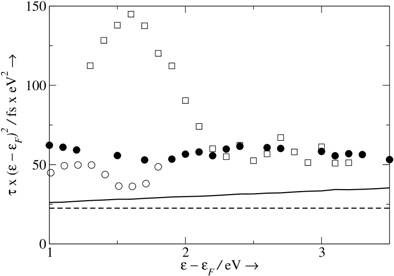
Figure 9: Experimental lifetimes of hot electrons in Cu, multiplied by $(\varepsilon-\varepsilon_{F})^{2}$ and as a function of $(\varepsilon-\varepsilon_{F})$. The open circles represent the TR-2PPE measurements reported by Knoesel et al.knoesel for the lifetime of very-low-energy hot electrons in Cu(111). The TR-2PPE measurements reported by Ogawa et al.ogawa for the lifetime of hot electrons in Cu(110) are represented by open squares. For comparison, the ab initio calculations represented in Fig. 8 by solid circles are also represented in this figure (solid circles), together with the lifetimes of hot electrons in a FEG with $r_{s}=2.67$ (solid line) and the corresponding approximation of Eqs. (13) and (14) dashed line).

An inspection of Fig. 8 shows that when the $3d$ shell is assigned to the core ab initio calculations (dashed line) nearly coincide with the FEG prediction (solid line). This must be a consequence of the fact that band-structure effects in Cu are nearly entirely due to the presence of localized $d$ electrons. In the presence of $d$ electrons, there are obviously more states available for the creation of e-h pairs, and one might be tempted to conclude that $d$ electrons should yield an enhanced hot-electron decay, especially at the opening of the $d$-band scattering channel at about $2\,{\rm eV}$ below the Fermi level. Indeed, this is precisely the result of calculation (i) represented by squares, which is very close to the calculation reported by Ogawa et al..ogawa ; note4 Nevertheless, a full ab initio evaluation of ${\rm Im}\,\epsilon_{{\bf G},{\bf G}}({\bf q},\omega)$ yields the calculation (ii) represented by open circles; this shows that there is no coupling between $d$ and $sp$ electrons below and above the Fermi level and there is, therefore, little impact of $d$ electrons on the production of e-h pairs.note5 The key role that $d$ electrons play in the hot-electron decay is mainly due to screening effects. The presence of $d$ electrons gives rise to additional screening, thus increasing the lifetime of hot electrons for all excitation energies, as shown by the result of calculation (iii) represented by triangles which includes the screening of $d$ electrons in the ab initio evaluation of the denominator of Eq. (30). The screening of $d$ electrons is found to increase hot-lectron lifetimes by a factor of 3. Finally, differences between calculation (iii) (triangles) and the full ab initio calculation (solid circles), which are only visible at hot-electron excitation energies very near the Fermi level, are due to a combination of band-structure effects on the hot-electron initial and final $sp$ states above the Fermi level and crystalline local-field effects not included in Eq. (30).

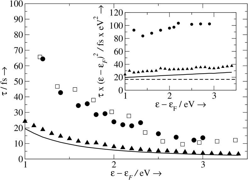
Figure 10: Hot-electron lifetimes in Au, as a function of the hot-electron energy $\varepsilon$ with respect to the Fermi level $\varepsilon_{F}$. Solid circles represent the ab initio RPA calculation, as obtained in Ref. campillo3 after averaging the lifetime broadening $\tau_{{\bf k},i}^{-1}$ of Eq. (26) over all states with the same energy $\varepsilon$. The open squares represent the experimental measurements of Ref. cao . The solid line represents the RPA lifetime of hot electrons in a FEG with $r_{s}=3.01$. The triangles represent the result obtained from Eq. (30) by replacing the hot-electron initial and final states entering the coefficients $B_{if}$ by plane waves and the dielectric function in $|\epsilon_{{\bf G},{\bf G}}({\bf q},\omega)|^{-2}$ by that of a FEG with $r_{s}=3.01$, but with full inclusion of the band structure in the calculation of ${\rm Im}\epsilon_{{\bf G},{\bf G}^{\prime}}({\bf q},\omega)$. The inset exhibits scaled lifetimes of hot electrons in Au. The solid circles and the solid line represent first-principles and FEG calculations, respectively, both within RPA. The dashed line represents the prediction of Eqs. (13) and (14). The triangles represent the result obtained from Eq. (30) by replacing the hot-electron initial and final states entering the coefficients $B_{if}$ by plane waves and the dielectric function in $|\epsilon_{{\bf G},{\bf G}}({\bf q},\omega)|^{-2}$ by that of a FEG with $r_{s}=3.01$, but with full inclusion of the band structure in the calculation of ${\rm Im}\epsilon_{{\bf G},{\bf G}^{\prime}}({\bf q},\omega)$.

The first time-resolved 2PPE (TR-2PPE) experiments on Cu were performed by Schmuttenmaer et al..schmu The electron dynamics on copper surfaces was later investigated by several groups.ogawa ; exp1 ; exp2 ; exp3 ; exp4 ; knoesel Although there were some discrepancies among the results obtained in different laboratories, most measured lifetimes were found to be much longer than those of hot electrons in a free gas of $4s^{1}$ valence electrons. The first-principles calculations reported in Ref. campillo1 (see also Fig. 8) indicate that this is mainly the result of the screening of $d$ electrons.

Fig. 9 exhibits (open circles) the TR-2PPE measurements reported by Knoesel et al.knoesel for the lifetime of very-low-energy electrons in Cu(111). Since the energy of these electrons is less than $\sim 2{\rm eV}$ above the Fermi level, $d$ electrons (the $d$-band threshold is located at $\sim 2\,{\rm eV}$ below the Fermi level) cannot participate in the creation of electron-hole pairs but can participate in the screening of e-e interactions, thereby increasing the hot-electron lifetime. Fig. 9 shows that the measurements of Knoesel et al. are in reasonable agreement with the first-principles calculations reported in Ref. campillo1 (solid circles). The relaxation dynamics at the low-index copper surfaces (111), (100), and (100) were investigated by Ogawa et al.ogawa in a wider energy range. Since the experiment detects the photoemitted electrons in the normal direction (${\bf k}_{\parallel}=0$), we have plotted in Fig. 9 (open squares) the measured lifetimes of hot electrons at the (110) surface of Cu, the only surface with no band gap for electrons emitted in this direction. At large electron energies ($\varepsilon-\varepsilon_{F}>2\,{\rm eV})$, there is very good agreement between calculated lifetimes (solid circles) and the measurements reported in Ref. ogawa (open squares). Nevertheless, the calculations cannot account for the large increase in the measured lifetimes reported in Ref. ogawa at lower electron energies. The origin of this discrepancy was discussed by Schöne et al.sc1 , who concluded that the increase in the experimentally determined lifetime might be related to the presence of a photohole below the Fermi level leading to transient excitonic states.

Ab initio RPA average lifetimes in Au, as reported in Ref. campillo3 , are represented in Fig. 10 (solid circles), together with accurate TR-2PPE measurements (open squares) where the relaxation from electron transport to the surface was expected to be negligible.cao This figure shows that there is very good agreement between theory and experiment, which are both found to be nearly five times larger than the lifetime of hot electrons in a free gas of $6s^{1}$ valence electrons (solid line). Nevertheless, more accurate linearized augmented plane-wave (LAPW)claudia and plane-waveidoia calculations of the lifetime of hot electrons in Au have been carried out recently, which yield smaller lifetimes than those reported in Ref. campillo3 and represented in Fig. 10 by an overall factor of $\sim 1.4$. These calculations have been found to accurately reproduce the BEES spectra for the two prototypical Au/Si and Pd/Si systemsclaudia .

The triangles of Fig. 10 show the result obtained in Ref. campillo3 from Eq. (30) (thus neglecting crystalline local-field effects) by including the actual band structure of Au in the evaluation of ${\rm Im}\,\epsilon_{{\bf G},{\bf G}}({\bf q},\omega)$ but treating the coefficients $B_{i,f}$ and the denominator $\left|\epsilon_{{\bf G},{\bf G}}({\bf q},\omega)\right|^{2}$ as in the case of a FEG with $r_{s}=3.01$. The result of this calculation is very close to the FEG calculation (solid lines), which shows that the opening of the $d$-band scattering channel for e-h pair production does not play a role. As in the case of Cu, differences between the FEG and the full ab initio calculation are mainly a consequence of virtual interband transitions due to the presence of $d$ electrons, which give rise to additional screening and largely increase the hot-electron lifetime in Au.

The change $\delta\epsilon$ in the real part of the long-wavelength dielectric function that is due to the presence of $d$ electrons in the noble metals is known to be practically constant at the low frequencies involved in the decay of low-energy hot electrons in these materials.eh1 ; eh2 ; eh3 Hence, in order to investigate hot-electron lifetimes and mean free paths in the noble metals Quinnquinn63 treated the FEG as if it were embedded in a medium of dielectric constant $\epsilon_{0}=1+\delta\epsilon$ instead of unity. The corrected lifetime is then found to be larger by a factor of $\epsilon_{0}^{1/2}$, i.e., $\sim 2.5$ for both Cu and Au. A more accurate analysis has been carried out recently, in which the actual frequency dependence of $\epsilon_{0}$ is included,aran showing that for the low energies of interest the corrected lifetime is still expected to be enhanced by a factor of $\sim 2.5$ for both Cu and Au. Nevertheless, the ab initio calculations exhibited in Figs. 9-11 indicate that the role that occupied $d$ states play in the screening of $e$-$e$ interactions is much more important in Au than in Cu.

Finally, we note that the screening of $d$ electrons does not depend on whether the hot electron can excite $d$ electrons (both in Cu and Au the $d$-band scattering channel opens at $\sim 2\,{\rm eV}$ below the Fermi level) or not. Thus, $d$-screening effects do not depend on the hot-electron energy, and average lifetimes are therefore expected to approximately scale as $(\varepsilon-\varepsilon_{F})^{-2}$, as in the case of a FEG. Nonetheless, departures from this scaling behaviour can occur when the hot-electron lifetimes are measured along certain symmetry directions, as discussed in Ref. campillo1

III.4.2 Linear muffin-tin orbital (LMTO) basis

For noble and transition metals containing $d$ and $f$ electrons it is sometimes more convenient to perform full all-electron calculations based on the use of localized basis like linear muffin-tin orbital (LMTO),andersen linear combination of atomic orbital (LCAO),lcao or LAPW basis.singh The lifetime of hot electrons in the noble metals Cu, Ag, and Au, and the $4d$ transition metals Nb, Mo, Rh, and Pd was determined by Zhukov et al.zhukov1 ; zhukov2 by using an LMTO basis in the so-called atomic-sphere approximation (ASA), in which the Wigner-Seitz (WS) cells are replaced by overlapping spheres.

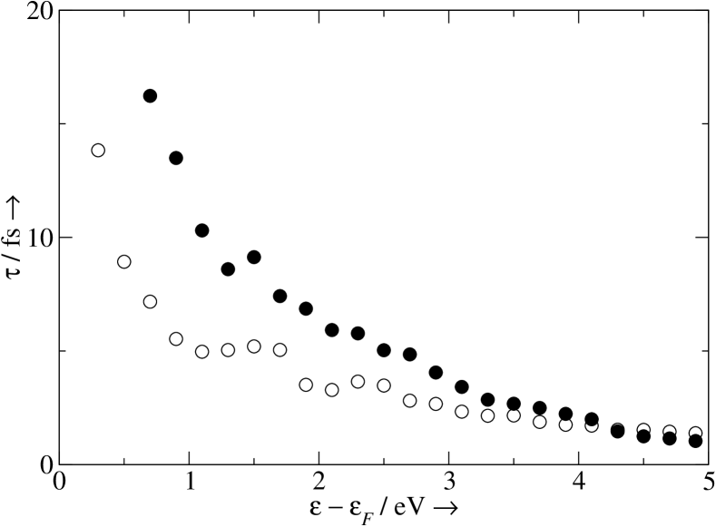
Figure 11: Hot-electron lifetimes in Nb and Pd, as a function of the hot-electron energy $\varepsilon$ with respect to the Fermi level $\varepsilon_{F}$. Solid and open circles represent ab initio RPA calculations for Nb and Pd, respectively, as obtained after averaging the lifetime broadening $\tau_{{\bf k},i}^{-1}$ of Eq. (26) over all states with the same energy $\varepsilon$.

In the LMTO method, one-electron Bloch states are expanded as follows

$$\phi_{{\bf k},i}({\bf r})=\sum_{{\bf R},L}u_{{\bf k},i}({\bf R},L)\,\chi_{{\bf R},L}({\bf r},{\bf k}),$$ (33)

where $L=(l,m)$ represents the angular momentum and $\chi_{{\bf R},L}({\bf r},{\bf k})$ are the LMTO basis wave functions, which in the ASA are constructed from the solutions $\varphi_{{\bf R},l}(r)$ to the radial Schrödinger equation inside the overlapping muffin-tin sphere at site ${\bf R}$ and their energy derivatives. Hot-electron reciprocal lifetimes can then be evaluated from Eqs. (26)-(29) by first solving self-consistently for the coefficients $u_{{\bf k},i}({\bf R},L)$ the Kohn-Sham equation of DFT with the use of the LDA for exchange and correlationperdew and then computing the dielectric matrix $\epsilon_{{\bf G},{\bf G}^{\prime}}({\bf q},\omega)$ from first principles.

In Fig. 11 we plot the ab initio RPA calculations that we have carried out from Eqs. (26)-(29) for the average lifetime $\tau(\varepsilon)$ [see Eq. (31)] of hot electrons in the body-centered-cubic (bcc) Nb and the fcc Pd. Nb ($4d^{4}5s^{1}$) is a transition metal with a partially filled $4d$ band and one $5s$ valence electron per atom. In this material, the bands of $d$ states lie in the energy interval from $4\,{\rm eV}$ below to $6\,{\rm eV}$ above the Fermi level. Hence, contrary to the case of the noble metals where hot electrons decay by promoting $sp$ electrons from below to above the Fermi level, in the case of Nb and other transition metals $d$ electrons also participate in the creation of e-h pairs. Accordingly, the net impact of $d$ electrons in the decay of hot electrons in Nb will be the result of the competition between the opening of a new scattering channel and the presence of $d$-electron screening. Valence ($5s^{1}$) electrons in Nb form a FEG with electron-density parameter $r_{s}=3.07$. However, the actual lifetimes of hot electrons in Nb are considerably shorter than those of hot electrons in the free gas of $5s^{1}$ valence electrons, which is obviously due to the presence of $d$ electrons. Furthermore, if one naively considered a FEG with 5 valence electrons per atom ($r_{s}=1.80$), one would predict a lifetime that is $\sim(3.07/1.80)^{5/2}\sim 4$ times larger [see Eq. (14)] than in the case of a FEG with $r_{s}=3.07$ and nearly 8 times larger than predicted by our ab initio calculation. On the one hand, $d$ electrons below and above the Fermi level in real Nb strongly couple for the creation of e-h pairs, thereby strongly decreasing the hot-electron lifetime for all electron energies under consideration. On the other hand, screening of localized $d$ electrons is much weaker than in the case of free electrons. Hence, while screening effects dominate in the case of a FEG, the effect of the DOS near the Fermi level dominates in the case of a gas of electrons with a large number of $d$ states, which yields the short average lifetimes plotted in Fig. 11.

Pd ($4d^{10}$) is a transition metal with a filled $4d$ band and no valence $sp$ electrons. In this material, the bands of $d$ states mainly lie below the Fermi level, though states above the Fermi level still have a small but significant $d$ component. The average density of 10 electrons per atom in Pd is higher than that of 5 electrons per atom in Nb; a FEG picture of the hot-electron dynamics in these materials would, therefore, lead to longer lifetimes in Pd. Nevertheless, our ab initio calculations show that in the case of low-energy electrons with energies below $4\,{\rm eV}$ this is not the case, i.e., hot electrons in Pd live shoter than in Nb. This is again due to the fact that as far as $d$ electrons are concerned the effect of the density of $d$ states near the Fermi level shortening the lifetime is more important than the effect of $d$-screening increasing the lifetime, simply because of the limited ability of $d$ electrons to screen the e-e interactions. The density of $d$ states near the Fermi level is higher in Pd than in Nb, thereby leading to lifetimes of low-energy electrons that are shorter in Pd than in Nb. At energies $\varepsilon-\varepsilon_{F}>4\,{\rm eV}$ e-h pair production is restricted to the lowest energies, due to the fact that for the highest energies $d$ electrons below the Fermi level do not couple with $sp$ electrons at a few eVs above the Fermi level. Thus, at these energies e-h pair production in Pd is not as efficient as in the case of Nb, which yields hot-electron lifetimes that are larger in Pd than in Nb.

IV Green function formalism

In the theoretical framework of section II we have restricted our analysis to the case of an external excited electron interacting with a Fermi system of $N$ interacting electrons. Nevertheless, a more realistic analysis should include the excited hot electron as part of one single Fermi system of $N+1$ interacting electrons in which an electron has been added in the one-particle state $\phi_{i}({\bf r})$ at time $t^{\prime}$. In the framework of Green function theory,hedin the probability that an electron will be found in the same one-particle state at time $t>t^{\prime}$ is obtained from the knowledge of the one-particle Green function of a system of $N$ interacting electrons. One finds,nekovee

$$P_{i}(t^{\prime},t)=\exp\left[2\,{\rm Im}E_{i}\,(t-t^{\prime})\right],$$ (34)

$\varepsilon_{i}$ being the so-called quasiparticle energy, i.e., the pole of the Green function. Hence, the total decay rate or reciprocal lifetime of the quasiparticle is simply

$$\tau_{i}^{-1}=-2\,{\rm Im}E_{i}.$$ (35)

The quasiparticle energy $E_{i}$ can be approximately expressed in terms of the electron self-energy [$\Sigma({\bf r},{\bf r}^{\prime};E_{i})$] and the eigenfunctions [$\phi_{i}({\bf r})$] and eigenvalues [$\varepsilon_{i}$] of an effective single-particle hamiltonian [$H=-\nabla_{\bf r}^{2}/2+V({\bf r})$]:rev2

$$E_{i}\approx\varepsilon_{i}+\Delta\Sigma(E_{i}),$$ (36)

where

$$\Delta\Sigma(E_{i}) = \int d{\bf r}\int d{\bf r}^{\prime}\phi_{i}^{*}({\bf r})\left[\Sigma({\bf r},{\bf r}^{\prime};E_{i})\right.$$ (37)

$$- \left.V({\bf r})\delta({\bf r}-{\bf r}^{\prime})\right]\phi_{i}({\bf r}^{\prime}).$$ (39)

The total decay rate or reciprocal lifetime of the quasiparticle can, therefore, be obtained as follows

$$\tau_{i}^{-1} = -2\,{\rm Im}\Delta\Sigma(E_{i})$$ (40)

$$= -2\,\int d{\bf r}\int d{\bf r}^{\prime}\phi_{i}^{*}({\bf r}){\rm Im}\Sigma({\bf r},{\bf r}^{\prime};E_{i})\phi_{i}({\bf r}^{\prime}).$$ (42)

Within many-body perturbation theory,fetter it is possible to obtain the electron self-energy $\Sigma({\bf r},{\bf r}^{\prime};E_{i})$ as a series in the bare Coulomb interaction $v({\bf r},{\bf r}^{\prime})$, but due to the long range of this interaction such a perturbation series contains divergent contributions. Therefore, the electron self-energy is usually rewritten as a series in the time-ordered screened interaction $W^{TO}({\bf r},{\bf r}^{\prime};\omega)$, which can be built from the knowledge of the Green function itself and coincides for positive frequencies ($\omega>0$) with the retarded screened interaction of Eq. (2). In the RPA, the Green function entering the screened interaction $W^{TO}({\bf r},{\bf r}^{\prime};\omega)$ is replaced by its noninteracting counterpart and for positive frequencies one simply finds Eq. (2) with the density-response function of Eq. (12).

To lowest order in the screened interaction, the self-energy $\Sigma({\bf r},{\bf r}^{\prime};E_{i})$ is obtained from the product of the Green function and the screened interaction, and is therefore called the $GW$ self-energy. If one further replaces both the Green function $G({\bf r},{\bf r}^{\prime};\omega)$ and the quasiparticle energy $E_{i}$ entering the GW self-energy by their noninteracting counterparts [$\Delta\Sigma(E_{i})\to\Delta\Sigma^{0}(\varepsilon_{i})$], Eq. (40) is easily found to yield an expression for the decay rate which exactly coincides with the decay rate dictated by Eqs. (1)-(3). This is the so-called on-shell $G^{0}W$ approximation, which within RPA is usually called the on-shell $G^{0}W^{0}$ approximation. There are various ways of going beyond this approximation, by either normalizing the electron energy, introducing short-range xc effects, or by looking at the so-called spectral function within a non-selfconsistent or a selfconsistent scheme for the Green function.

IV.1 Electron-energy renormalization

Near the energy shell, i.e., assuming that the deviation of the complex quasiparticle energy $E_{i}$ from its noninteracting counterpart $\varepsilon_{i}$ is small, $E_{i}$ can be expanded as follows

$$E_{i}\approx\varepsilon_{i}+\Delta\Sigma(\varepsilon_{i})+(E-\varepsilon_{i})\,\left.{\partial\Delta\Sigma(\omega)\over\omega}\right|_{\omega=\varepsilon_{i}}.$$ (43)

This expansion yields

$$E_{i}\approx\varepsilon_{i}+Z(\varepsilon_{i})\,\Delta\Sigma(\varepsilon_{i}),$$ (44)

where $Z$ is the complex quasiparticle weight or renormalization factor:

$$Z(\varepsilon_{i})=\left[1-\left.{\partial\Delta\Sigma(\omega)\over\omega}\right|_{E=\varepsilon_{i}}\right]^{-1}.$$ (45)

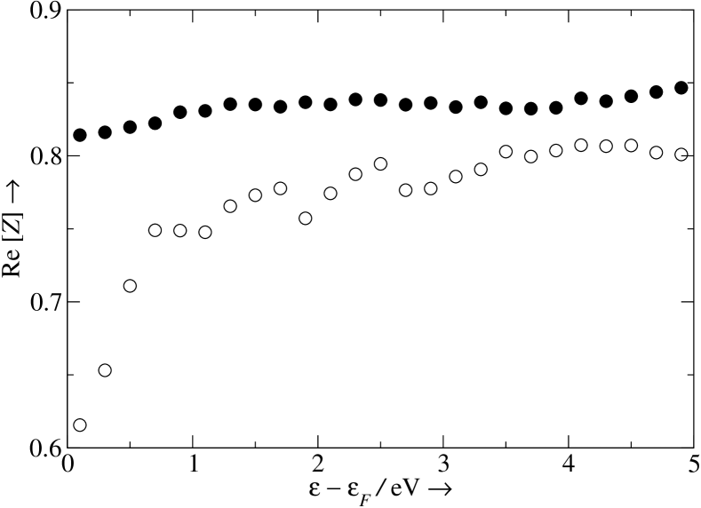
Figure 12: The real part of the renormalization factor $Z(\varepsilon_{i})$ of Eq. (45), versus $\varepsilon_{i}-\varepsilon_{F}$, as obtained from a first-principles evaluation of the $G^{0}W^{0}$ electron self-energy in Cu (open circles) and Pd (crosses).

RPA calculations of the renormalization factor $Z(\varepsilon_{i})$ of a FEG were performed by Hedin.hedin0 These calculations show that in the case of a free gas of interacting electrons the renormalization factor near the Fermi level varies from unity in the high-density ($r_{s}\to 0$) limit to $\sim 0.6$ at $r_{s}=6$, the imaginary part being very small. We have carried out first-principles RPA calculations of the renormalization factor of a variety of real solids. We have found that as in the case of a FEG at metallic densities ($r_{s}=2-6$) this factor varies near the Fermi level from $\sim 0.8$ to $\sim 0.6$, as shown in Fig. 12 where the real part of the renormalization factor $Z(\varepsilon_{i})$ of Cu and Pd is represented versus the noninteracting electron energy $\varepsilon_{i}$.

Introducing Eq. (44) into Eq. (35), one finds

$$\tau_{i}^{-1}=-2\left[{\rm Re}Z(\varepsilon_{i}){\rm Im}\Delta\Sigma(\varepsilon_{i})+{\rm Im}Z(\varepsilon_{i}){\rm Re}\Delta\Sigma(\varepsilon_{i})\right].$$ (46)

Since the imaginary part of the renormalization factor $Z(\varepsilon_{i})$ is typically very small, Eq. (46) yields quasiparticle lifetimes that are larger than those obtained on-the-energy-shell by $\sim 30-40\%$. However, one must be cautious with the use of Eq. (46) when the self-energy is calculated in the $G^{0}W$ approximation by replacing the electron Green function by its noninteracting counterpart, which is built from the single-particle wave functions $\phi_{i}({\bf r})$ and energies $\varepsilon_{i}$ In this approximation, it should be more appropriate to evaluate the self-energy on-shell by also replacing $E_{i}$ by $\varepsilon_{i}$ in the calculation of the self-energy. This on-shell approximation yields a lifetime broadening of the form of Eq. (46) with $Z(\varepsilon_{i})=1$, which exactly coincides with the decay rate dictated by Eqs. (1)-(3).

IV.2 $GW\Gamma$ approximation

Exchange and short-range correlation of the excited hot electron with the Fermi system, which are absent in the $G^{0}W$ approximation, can be included in the framework of the $GW\Gamma$ approximation.mahan1 ; mahan2 In this approximation, the electron self-energy is of the $GW$ form, but with the actual time-ordered screened interaction $W^{TO}({\bf r},{\bf r}^{\prime};\omega)$ replaced by an effective screened interaction $\tilde{W}^{TO}({\bf r},{\bf r}^{\prime};\omega)$ which for $\omega>0$ is obtained as follows

$$\tilde{W}({\bf r},{\bf r}^{\prime};\omega)=v({\bf r},{\bf r}^{\prime})+\int d{\bf r}_{1}d{\bf r}_{2}\left[v({\bf r},{\bf r}_{1})\right.$$ (47)

(48)

$$+\left.f_{xc}({\bf r},{\bf r}_{1};\omega)\right]\chi({\bf r}_{1},{\bf r}_{2};\omega)v({\bf r}_{2},{\bf r}^{\prime}),$$ (49)

the density-response function $\chi({\bf r},{\bf r}^{\prime};\omega)$ now being

$$\chi({\bf r},{\bf r}^{\prime};\omega)=\chi^{0}({\bf r},{\bf r}^{\prime};\omega)+\int d{\bf r}_{1}\int d{\bf r}_{2}\,\chi^{0}({\bf r},{\bf r}_{1};\omega)$$ (50)

(51)

$$\times\left[v({\bf r}_{1},{\bf r}_{2})+f_{xc}({\bf r},{\bf r}_{1};\omega)\right]\,\chi({\bf r}_{2},{\bf r}^{\prime};\omega).$$ (52)

The kernel $f_{xc}({\bf r},{\bf r}_{1};\omega)$ entering Eqs. (47) and (50), which equals the second functional derivative of the xc energy functional $E_{xc}[n({\bf r})]$, accounts for the reduction in the electron-electron interaction due to the existence of short-range xc effects associated with the excited quasiparticle and with screening electrons, respectively. In the so-called time-dependent local-density approximation (TDLDA)soven or, equivalently, adiabatic local-density approximation (ALDA), the exact xc kernel is replaced by

$$f_{xc}^{ALDA}({\bf r},{\bf r}^{\prime};\omega)=\left.{d^{2}\left[n\varepsilon_{xc}(n)\right]\over dn^{2}}\right|_{n=n({\bf r})}\delta({\bf r}-{\bf r}^{\prime}),$$ (53)

where $\varepsilon_{xc}(n)$ is the xc energy per particle of a uniform electron gas of density $n$, and $n({\bf r})$ is the actual electron density at point ${\bf r}$.

Introduction of the $GW\Gamma$ self-energy into Eq. (40) yields on-the-energy-shell ($E_{i}\to\varepsilon_{i}$) an expression for the decay rate of the form of Eqs. (1)-(3) with the screened interaction $W({\bf r},{\bf r}^{\prime};\omega)$ of Eq. (2) replaced by that of Eq. (47). Existing first-principles calculations of hot-electron lifetimes in solids have all been carried out by neglecting short-range xc effects, i.e., by taking $f_{xc}({\bf r},{\bf r}^{\prime};\omega)=0$ in Eqs. 47 and 50. First-principles calculations with full inclusion of short-range xc effects have been performed only very recently.idoia

IV.3 Spectral function

In the framework of many-body theory, the propagation and damping of an excited electron (quasiparticle) in the one-particle state $\phi_{i}({\bf r})$ are dictated by the peaks in the spectral function $A_{i}(\omega)$, which is closely related to the imaginary part of the one-particle Green function $G({\bf r},{\bf r}^{\prime};\omega)$:hedin

$$A_{i}(\omega)={1\over\pi}\int d{\bf r}\int d{\bf r}^{\prime}\phi_{i}^{*}({\bf r}){\rm Im}G({\bf r},{\bf r}^{\prime};\omega)\phi_{i}({\bf r}^{\prime}),$$ (54)

where

$$G^{-1}({\bf r},{\bf r}^{\prime};\omega) = G_{0}^{-1}({\bf r},{\bf r}^{\prime};\omega)$$ (55)

$$- \left[\Sigma({\bf r},{\bf r}^{\prime};\omega)-V({\bf r})\,\delta({\bf r},{\bf r}^{\prime})\right].$$ (57)

The noninteracting Green function $G_{0}({\bf r},{\bf r}^{\prime};\omega)$ is obtained from the eigenfunctions [$\phi_{i}({\bf r})$] and eigenvalues [$\varepsilon_{i}$] of an effective single-particle hamiltonian [$H=-\nabla_{\bf r}^{2}/2+V({\bf r})$].

The energetic position of the peak in the spectral function defines the real part of the quasiparticle energy. The damping rate or lifetime broadening of the quasiparticle is given by the full width at half maximum (FWHM) $\Delta_{i}$ of the peak:

$$\tau_{i}^{-1}=\Delta_{i}.$$ (58)

Assuming that the peak in the spectral function $A_{i}(\omega)$ has a symmetric Lorentzian form, this definition of the damping rate coincides with the decay rate dictated by Eq. (35).

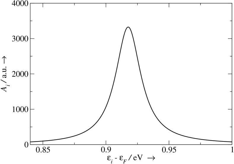
Figure 13: Spectral function of an excited electron at the $W$ point in Al ($\varepsilon_{i}=1.02\,{\rm eV}$), versus $\varepsilon_{i}-\varepsilon_{F}$, as obtained from Eq. (54) in the $G^{0}W^{0}$ approximation.

We have carried out first-principles $G^{0}W^{0}$ calculations of the spectral function in Al. For an excited electron at the $W$ point with energy $\varepsilon_{i}=1.02{\rm eV}$ above the Fermi level, we have found the spectral function represented in Fig. 13. This figure shows that the spectral function has indeed a single well-defined quasiparticle peak at the quasiparticle energy $\varepsilon_{qp}=0.92\,{\rm eV}$ above the Fermi level with the FWHM $\Delta_{i}=24\,{\rm meV}$ corresponding to the quasiparticle lifetime $\tau=27\,{\rm fs}$. Similar calculations were performed by Schöne et al.ekardt for various one-particle Bloch excited states in the simple metal Al and the noble metals Cu, Ag, and Au. These authors found hot-electron lifetimes that are in reasonable agreement with the $G^{0}W^{0}$ calculations obtained by Campillo et al.campillo1 ; campillo2 ; campillo3 from Eq. (40).

Full self-consistent $GW$ self-energy calculations, where the interacting Green function $G({\bf r},{\bf r}^{\prime};\omega)$ of Eq. (55) is used self-consistently to evaluate both the screened interaction and the $GW$ self-energy, have been carried out recently for the FEGvonbarth and simple semiconductorseguiluz1 ; eguiluz2 . Although self-consistency is nowadays known to yield very accurate total energies, existing calculations tend to indicate that non-self-consistent calculations should be preferred for the study of quasiparticle dynamics.vonbarth ; eguiluz1 This is due to the fact that vertex corrections not included in the self-consistent $GW$ self-energy might cancel out the effect of self-consistency, thereby full self-consistent self-energy calculations that go beyond the $GW$ approximation yielding results that might be close to $G^{0}W^{0}$ calculations.

V Summary and Conclusions

We have presented a survey of current theoretical investigations of the ultrafast electron dynamics in metals.

First of all, a theoretical description of the finite inelastic lifetime of excited hot electrons in a many-electron system has been outlined, in the framework of time-dependent perturbation theory. Then, the main factors that determine the decay of excited states have been discussed, and the existing first-principles theoretical investigations of the lifetime of hot electrons in the bulk of a variety of metals have been reviewed and compared to the available experimental data. The decay rates obtained within first-order time-dependent perturbation theory have been shown to coincide with the on-shell $G^{0}W^{0}$ approximation of many-body theory and to provide a suitable framework to explain most of the available experimental data for simple and noble metals.

Finally, various ways of going beyond the $G^{0}W^{0}$ approximation have been discussed, by normalizing the electron energy, introducing short-range xc effects, or looking at either the $G^{0}W^{0}$ or the self-consistent $GW$ spectral function. First-principles $GW\Gamma$ calculations with full inclusion of short-range xc effects have been carried out only very recently.idoia

Alternatively, nonperturbative treatments of the interaction of external excited electrons with a Fermi system have been developed.nagy ; nazarov These treatments are based on phase-shift calculations from kinetic theorynagy and a modification of the Schwinger variational principle of scattering theory,nazarov both implemented for electrons in a FEG. The role of spin fluctuations in the screening and the scattering of excited electrons in a FEG has also been discussednagy2 in the framework of kinetic theory, with the use of simple physically motivated models.

The experiments considered here all involve very low densities of excited electrons, and the mutual interaction of excited electrons have been completely neglected in the theoretical calculations. In a situation in which the density of excited electrons is high, a different theoretical approach would be needed. Calculations along these lines have been carried out by Knorren et al.,knorren ; knorren2 by solving the Boltzmann equation for carriers in the conduction band.

- (1) R. Haight, Surf. Sci. Rep. 1995, 21, 275.
- (2) M. Wolf, G. Ertl, Science 2000, 288, 1352.
- (3) H. Nienhaus, Surf. Sci. Rep. 2002, 45, 1.
- (4) G. Grimvall, in: E. P. Wohlfarth (Ed.), The Electron-Phonon Interaction in Metals, Selected Topics in Solid State Physics, Vol. 16, North-Holland, Amsterdam, 1981.
- (5) A. Eiguren, B. Hellsing, G. Nicolay, E. V. Chulkov, V. M. Silkin, S. Hüfner, P. M. Echenique, Phys. Rev. Lett. 2002, 88, 66805.
- (6) J. C. Fuggle, J. E. Inglesfield (Eds.), Unoccupied Electronic States, Topics in Applied Physics, Vol. 69, Springer, Berlin, 1992.
- (7) R. Matzdorf, Surf. Sci. Rep. 1998, 30, 153.
- (8) Th. Fauster, W. Steinmann, in: P. Halevi (Ed.), Electromagnetic Waves: Recent Developments in Research, Elsevier, Amsterdam, 1994.
- (9) H. Petek, S. Ogawa, Prog. Surf. Sci. 1997, 56, 239.
- (10) J. Li, W.-D. Schneider, R. Berndt, O. R. Bryant, S. Crampin, Phys. Rev. Lett. 1998, 81, 4464.
- (11) L. Burgi, O. Jeandupeux, H. Brune, K. Kern, Phys. Rev. Lett. 1999, 82, 4516.
- (12) J. Kliewer, R. Berndt, E. V. Chulkov, V. M. Silkin, P. M. Echenique, S. Crampin, Science 2000, 288, 1399.
- (13) K. Reuter, U. Hohenester, P. L. de Andrés, F. J. García-Vidal, F. Flores, K. Heinz, P. Kocevar, Phys. Rev. B 2000, 61, 4522.
- (14) F. Ladstädter, P. F. de Pablos, U. Hohenester, P. Pusching, C. Ambrosch-Draxl, P. L. de Andrés, F. J. García-Vidal, F. Flores, Phys. Rev. B 2003, 68, 85107.
- (15) P. M. Echenique, J. M. Pitarke, E. V. Chulkov, V. M. Silkin, J. Electron Spectrosc. 2002, 126, 163.
- (16) R. H. Ritchie, F. W. Garber, M. Y. Nakai, R. D. Birkhoff, in: L. G. Augenstein, R. Mason, M. Zelle (Eds.), Advances in Radiation Biology, Vol. 3, Academic Press, New York, 1969.
- (17) P. M. Echenique, J. M. Pitarke, E. V. Chulkov, A. Rubio, Chem. Phys. 2000, 251, 1.
- (18) I. Campillo, J. M. Pitarke, A. Rubio, E. Zarate, P. M. Echenique, Phys. Rev. Lett. 1999, 83, 2230.
- (19) W.-D. Schöne, R. Keyling, M. Bandić, W. Ekardt, Phys. Rev. B 60, 8616 1999; R. Keyling, W.-D. Schöne, W. Ekardt, Phys. Rev. B 2000, 61, 1670.
- (20) I. Campillo, V. M. Silkin, J. M. Pitarke, E. V. Chulkov, A. Rubio, P. M. Echenique, Phys. Rev. B 2000, 61, 13484.
- (21) I. Campillo, J. M. Pitarke, A. Rubio, P. M. Echenique, Phys. Rev. B 2000, 62, 1500.
- (22) J. M. Pitarke, I. Campillo, Nucl. Instrum. Methods B 2000, 164, 147.
- (23) A. L. Fetter, J. D. Wallecka, Quantum theory of Many Particle Systems (MacGraw-Hill, New York, 1964 ).
- (24) R. M. Dreizler, E. K. U. Gross, Density Functional Theory (Springer-Verlag, Berlin, 1990).
- (25) F. Aryasetiawan, O. Gunnarsson, Rep. Prog. Phys. 1998, 61, 237.
- (26) M. Nekovee, J. M. Pitarke, Comput. Phys. Commun. 2001, 137, 123.
- (27) In usual practice all single-particle wave functions and energies are typically obtained by solving the single-particle Kohn-Sham equation of density-functional theory in the so-called local-density approximation (LDA) [see, e.g., Ref. gross ].
- (28) W. Shockley, Phys. Rev. 1939, 56, 317.
- (29) P. O. Gartland, B. J. Slagsvold, Phys. Rev. B 1975 12, 4047.
- (30) W. Eberhardt, E. W. Plummer, Phys. Rev. B 1980, 21, 3245.
- (31) P. M. Echenique, J. B. Pendry, J. Phys. C 1978, 11, 2065; Prog. Surf. Sci. 1990, 32, 111.
- (32) N. V. Smith, Rep. Prog. Phys. 1988, 51, 1227.
- (33) E. V. Chulkov, I. Sarria, V. M. Silkin, J. M. Pitarke, P. M. Echenique, Phys. Rev. Lett. 1998, 80, 4947; J. Osma, I. Sarria, E. V. Chulkov, J. M. Pitarke, P. M. Echenique, Phys. Rev. B 1999, 59, 10591; I. Sarria, J. Osma, E. V. Chulkov, J. M. Pitarke, P. M. Echenique, Phys. Rev. B 1999, 60, 11795.
- (34) J. J. Quinn, R. A. Ferrell, Phys. Rev. 1958, 112, 812.
- (35) For and , one finds or, equivalently, .
- (36) J. Lindhard, K. Dan. Vidensk. Selsk. Mat.-Fys. Medd. 1954, 28, No. 8.
- (37) D. Pines, Elementary Excitations in Solids, (W. A. Benjamin, Inc., New York, 1963).
- (38) C. N. Berglund, W. E. Spicer, Phys. Rev. 1964, 136, A1030.
- (39) E. O. Kane, Phys. Rev. 1967, 159, 624.
- (40) W. F. Krolikowsky, W. E. Spicer, Phys. Rev. 1969, 185, 882.
- (41) D. R. Penn, S. P. Apell, S. M. Girvin, Phys. Rev. Lett. 1985, 55, 518; Phys. Rev. B 1985, 32, 7753.
- (42) D. R. Penn, S. P. Apell, Phys. Rev. B 1988, 38, 5051.
- (43) F. Passek, M. Donath, K. Ertl, V. Dose, Phys. Rev. Lett. 1995, 75, 2746.
- (44) H.-L. Drouhin, Phys. Rev. B 1997, 56, 14886; 2000, 62, 556.
- (45) E. Zarate, S. P. Apell, P. M. Echemique, Phys. Rev. B 1999, 60, 2326.
- (46) V. P. Zhukov, E. V. Chulkov, J. Phys.: Condens. Matter 2002, 14, 1937.
- (47) V. P. Zhukov, F. Aryasetiawan, E. V. Chulkov, P. M. Echenique, Phys, Rev. B 2002 65, 115116.
- (48) M. R. Bacelar, W.-D. Schöne, R. Keyling, W. Ekardt, Phys. Rev. B 2002, 66, 153101.
- (49) D. Ceperley, B. J. Alder, Phys. Rev. Lett. 45, 1196 1980, as parametrized by J. P. Perdew, A. Zunger, Phys. Rev. B 1981, 23, 5048.
- (50) N. Troullier, J. L. Martins, Phys. Rev. B 1991, 43, 1993.
- (51) I. Campillo, J. M. Pitarke, A. G. Eguiliz, A. García, Nucl. Instrum. Methods B 1998, 135, 103; I. Campillo, J. M. Pitarke, and A. G. Eguiluz, Phys. Rev. B 58, 19307 1998.
- (52) S. Ogawa, H. Nagano, H. Petek, Phys. Rev. B 1997, 55, 1.
- (53) Small differences between the results represented by a dashed line in Fig. 8 (see also Ref. campillo2 ) and those reported in Ref. ogawa are entirely due to the fact that the FEG dielectric function used in by Ogawa et al.ogawa was obtained within the static Thomas-Fermi approximation of Eq. (8). In the evaluation of the FEG , the electron-density parameter was taken from the actual DOS at the Fermi level in both Refs. campillo2 and ogawa .
- (54) A similar situation occurs in the decay of holes in Cu [see I. Campillo, A. Rubio, J. M. Pitarke, A. Goldmann, P. M. Echenique, Phys. Rev. Lett. 2000, 85, 3241; A. Gerlach, K. Berge, A. Goldmann, I. Campillo, A. Rubio, J. M. Pitarke, P. M. Echenique, Phys. Rev. B 2001, 64, 85423]. The small overlap between and states below the Fermi level is found to be responsible for a long lifetime of holes, especially at the top of the band where the hole can only couple with states below the Fermi level.
- (55) C. A. Schmuttenmaer, M. Aeschlimann, H. E. Elsayed-Ali, R. J. D. Miller, D. A. Mantell, J. Cao, Y. Gao, Phys. Rev. B 1994, 50, 8957.
- (56) M. Aeschlimann, M. Bauer, S. Pawlik, Chem. Phys. 1996, 205, 127.
- (57) T. Hertel, E. Knoesel, M. Wolf, G. Ertl, Phys. Rev. Lett. 1996, 76, 535.
- (58) S. Pawlik, M. Bauer, M. Aeschlimann, Surf. Sci. 1997, 377-379, 206.
- (59) J. Cao, Y. Gao, R. J. Miller, H. E. Elsayed, D. A. Mantell, Phys. Rev. B 1997, 56, 1099.
- (60) E. Knoesel, A. Hotzel, M. Wolf, Phys. Rev. B 1998, 57, 12812.
- (61) W.-D. Schöne, W. Ekardt, Phys. Rev. B 2000, 62, 13464; J. Phys.: Condens. Matter 2002, 14, 4669.
- (62) J. Cao, Y. Gao, H. E. Elsayed-Ali, R. J. D. Miller, D. A. Mantell, Phys. Rev. B 1998, 58, 10948.
- (63) H. Ehrenreich, H. R. Philipp, Phys. Rev. 1962, 128, 1622.
- (64) B. R. Cooper, H. Ehrenreich, H. R. Philipp, Phys. Rev. 1965, 138, A494.
- (65) P. B. Johnson, R. W. Christy, Phys. Rev. B 1972, 6, 4370.
- (66) J. J. Quinn, Appl. Phys. Lett. 1963, 2, 167.
- (67) A. García-Lekue, J. M. Pitarke, E. V. Chulkov, A. Liebsch, and P. M. Echenique, Phys. Rev. B 2003, 68, 45103.
- (68) O. K. Andersen, Phys. Rev. B 1975, 12, 3060.
- (69) N. W. Ashcroft, N. D. Mermin, Solid State Physics (Sauders College, Philadelphia, 1976).
- (70) D. J. Sing, Planewaves, Pseudopotentials, and the LAPW method (Kluwer Academic Publishers, Boston, 1994).
- (71) V. P. Zhukov, F. Aryasetiawan, E. V. Chulkov, I. G. Gurtubay, P. M. Echenique, Phys. Rev. B 2001, 64, 195122.
- (72) L. Hedin, S. Lundqvist, Solid State Phys. 1969, 23, 1.
- (73) L. Hedin, Phys. Rev. 1965, 139, A796.
- (74) G. D. Mahan, B. E. Sernelius, Phys. Rev. Lett. 1989, 62, 2718.
- (75) G. D. Mahan, Many-Particle Physics (Plenum, New York, 1990).
- (76) A. Zangwill, P. Soven, Phys. Rev. A 1981, 21, 1561.
- (77) I. G. Gurtubay, J. M. Pitarke, P. M. Echenique (unpublished).
- (78) B. Holm, U. von Barth, Phys. Rev. B 1998, 57, 2108; B. Holm, Phys. Rev. Lett. 1999, 83, 788.
- (79) W.-D. Schöne, A. G. Eguiluz, Phys. Rev. Lett. 1998, 81, 1662.
- (80) W. Ku, A. G. Eguiluz, Phys. Rev. Lett. 2002, 89, 126401.
- (81) I. Nagy, J. I. Juaristi, P. M. Echenique, Phys. Rev. B 2000, 63, 035102.
- (82) V. U. Nazarov, S. Nishigaki, J. M. Pitarke (unpublished).
- (83) I. Nagy, M. Alducin, J. I. Juaristi, P. M. Echenique, Phys. Rev. B 2001, 64, 075101.
- (84) R. Knorren, K. H. Bennemann, R. Burgermeister, M. Aeschlimann, Phys. Rev. B 2000, 61, 9427; R. Knorren, G. Bouzerar, K. H. Bennemann, J. Phys.: Condens. Matter 2002, 14, R379.
- (85) M. Aeschlimann, M.Bauer, S. Pawlik, R. Knorren, G. Bouzerar, and K. H. Bennemann, Appl. Phys. A 2000, 71, 485.