Reduction of $T_{\mathrm{c}}$ due to Impurities in Cuprate Superconductors

Abstract

In order to explain how impurities affect the unconventional superconductivity, we study non-magnetic impurity effect on the transition temperature using on-site $U$ Hubbard model within a fluctuation exchange (FLEX) approximation. We find that in appearance, the reduction of $T_{\mathrm{c}}$ roughly coincides with the well-known Abrikosov-Gor’kov formula. This coincidence results from the cancellation between two effects; one is the reduction of attractive force due to randomness, and another is the reduction of the damping rate of quasi-particle arising from electron interaction. As another problem, we also study impurity effect on underdoped cuprate as the system showing pseudogap phenomena. To the aim, we adopt the pairing scenario for the pseudogap and discuss how pseudogap phenomena affect the reduction of $T_{\mathrm{c}}$ by impurities. We find that ’pseudogap breaking’ by impurities plays the essential role in underdoped cuprate and suppresses the $T_{\mathrm{c}}$ reduction due to the superconducting (SC) fluctuation.

1 Introduction

Until now many experiments on the effect of impurity substitution in hole-doped cuprate high-$T_{\mathrm{c}}$ superconductors (HTS cuprates) have been done, and it is well known that the substitution in the copper site leads to a rapid $T_{\mathrm{c}}$ reduction. In their experiments, the following Abrikosov-Gor’kov (AG) formula [1] is usually used to analyse the dependence of $T_{\mathrm{c}}$ on impurity content :

$$\ln\left(\frac{T_{c}}{T_{c0}}\right)=\psi\left(\frac{1}{2}\right)-\psi\left(\frac{1}{2}+\frac{\Gamma}{2\pi T_{c}}\right),$$ (1)

where $\psi(x)$ is the digamma function, $T_{\mathrm{c0}}=T_{\mathrm{c}}(n_{\mathrm{imp}}=0)$, and $\Gamma$ is the pair breaking scattering rate. In most of experiments which study impurity effect in the HTS, fitting the measured data by Eq.(1) seems to be successful, especially in the low impurity concentration regime because of its linear bahavior. For example, it is reported theoretically and experimentally that the $T_{\mathrm{c}}$ reduction by Zn substitution in HTS follows quantitatively Eq.(1), where Zn is treated as a strong non-magnetic scatterer, and $\Gamma$ is evaluated in the unitarity limit. [2, 3, 4]

However, it is not so obvious that AG formula can be used to estimate impurity effects in HTS cuprates. The simplicity of Eq.(1) is based on the treatment of HTS as the weak-coupling $d$-wave BCS superconductor and the calculation technique of taking an average on Fermi surface. In such a treatment, the microscopic mechanism of superconducting pairing is not included at all, so the pairing interaction is not affected by impurities, whereas HTS is the typical system in which the pairing interaction is caused by Coulomb repulsion $U$ and the momentum dependence plays the essential role in the mechanism of superconductivity. Thus, the effect of impurity on the pairing interaction may not be negligible in HTS. Therefore, it is necessary to study how impurities suppresses $T_{\mathrm{c}}$ from the microscpic view. To clarify the reason why Eq.(1) represents $T_{\mathrm{c}}$ reduction in HTS cuprate is one of the purpose of this paper and discussed in $\S 3$.

As another problem, it is frequently debated that the impurity effect on underdoped cuprate is different from that on overdoped cuprate. In the experiments on the $T_{\mathrm{c}}$-reduction by copper site substitution, [11, 12] it has been noted that in underdoped regime there is more rapid reduction of $T_{\mathrm{c}}$ than in the overdoped regime. In the other kind of experiments on electron irradiated samples, it is reported that the variation of $T_{\mathrm{c}}$ with defect content in underdoped and optimally doped $\mathrm{Y}\mathrm{Ba}_{\mathrm{2}}\mathrm{Cu}_{\mathrm{3}}\mathrm{O}_{\mathrm{7-\delta}}$ is quite linear and contrasts with the AG formula. Because one of the feature of underdoped cuprate in the clean samples is the pseudogap phenomena, it is natural to consider that such remarkable behaviors in underdoped region originate from the pseudogap. Therefore, we disscuss how pseudogap phenomena affect the reduction of $T_{\mathrm{c}}$ by impurities. This is the second purpose of this paper and is discussed in $\S 4$.

Through this study, we treat impurities as non-magnetic ones in the mind of the Zn-substitution and defects; We assume that the scattering is elastic and that the impurity potential is the form of $\delta$-function type and we take an average on the positions of impurities. Moreover, we take the unitarity limit.

This paper is constructed in the following way. In $\S 2$, we consider the impurity effect in the weak-coupling $d$-wave BCS model. We point out that $T_{\mathrm{c}}$ reduction in the model almost coincides with AG formula and that the slight deviation from the AG curve originates from the direct momentum summation done numerically. In $\S 3$, using the FLEX approximation, we discuss $T_{\mathrm{c}}$ reduction by impurities in the system where the pairing interaction is caused by $U$. First, we introduce the FLEX theory and our theorical treatment for impurities. In $\S 3.2$, we show how impurities affect the main factors to determine the value of $T_{\mathrm{c}}$. In $\S 3.3$, we discuss the coincidence between the obtained $T_{\mathrm{c}}$ reduction and AG formula and we explain the reason. In $\S 3.4$, we point out the necessity of our treatment for the impurity effect in the HTS. In $\S 4$, using ’pairing scenario’, we discuss how pseudogap phenomena affect $T_{\mathrm{c}}$ reduction due to impurities in the mind of the disordered underdoped cuprate. We first review the theorical treatment in the pairing scenario. In $\S 4.2$, we include impurity effect in the theory and show some features of $T_{\mathrm{c}}$ reduction in the presence of pseudogap. We point out that such features are caused by ’pseudogap breaking’. In $\S 4.3$, we explain what the ’pseudogap breaking’ is. Finally, we shortly comment on the quantum dynamics of SC fluctuation. In the last section $\S 5$, we conclude the whole discussion.

2 Reduction of $T_{\mathrm{c}}$ by impurities in the weak-coupling $d$-wave BCS model

In this section, we consider non-magnetic impurity effect on $T_{\mathrm{c}}$ reduction in the unitarity limit within the weak-coupling $d$-wave BCS model. We assume the following separable attractive interaction:

$$V_{\mathbf{k,k^{\prime}}}=-g\varphi_{\mathbf{k}}\varphi_{\mathbf{k^{\prime}}},$$ (2)

where $g>0$ is the strength of the interaction and $\varphi_{\mathbf{k}}=\cos k_{x}-\cos k_{y}$, the form factor of $d_{\mathrm{x^{2}-y^{2}}}$-wave. The transition temperature is determined by

$$1=-\frac{1}{\beta N}\sum_{\mathbf{k},n}V_{\mathbf{k},\mathbf{k}}G(\mathbf{k},i\omega_{n})G(-\mathbf{k},-i\omega_{n}),$$ (3)

where

$$G(\mathbf{k},i\omega_{n})=[i\omega_{n}-(\epsilon_{\mathbf{k}}-\mu)-\Sigma_{\mathrm{imp}}(i\omega_{n})]^{-1}$$ (4)

with

$$\Sigma_{\mathrm{imp}}(i\omega_{n})=-\frac{n_{\mathrm{imp}}}{\frac{1}{N}\sum_{\mathbf{k}}G(\mathbf{k},i\omega_{n})}.$$ (5)

We numerically solve these equations. Here $\mu$ is the chemical potential, $\omega_{n}$ is the fermionic Matubara frequency, $\omega_{n}=(2n+1)\pi T$, and $n_{\mathrm{imp}}$ is the impurity concentration. We consider the 2D square lattice and assume the following tight-binding dispersion

$$\epsilon_{\mathbf{k}}=-2t(\cos k_{x}+\cos k_{y})+4t^{\prime}\cos k_{x}\cos k_{y}.$$ (6)

The filling of electrons is represented by $n$, and $n=1$ corresponds to the half filling. The parameters are chosen as $2t=1$, $t^{\prime}/t=0.25$, $g=0.7t$ and $n=0.75\sim 0.90$. The Fermi surfaces of bare electrons with dispersion Eq. (6) and the density of state (DOS), $\rho(w)=-\frac{1}{\pi}\sum_{\mathbf{k}}\mathrm{Im}G(\mathbf{k},\omega)$, are shown in Fig. 1. Here, $\omega=0$ is the Fermi level.

When we assume the particle-hole symmetry and replace the momentum summation with the Fermi surface average in calculating Eqs.(3)-(5), we obtain the well-known AG formula, Eq.(1), with the pair-breaking parameter $\Gamma=\frac{n_{\mathrm{imp}}}{\pi\rho(0)}$. [2, 4] The critical impurity concentration $n_{\mathrm{imp}}^{\mathrm{c}}$ is given by $n_{\mathrm{imp}}^{\mathrm{c}}=\frac{\pi^{2}\rho(0)T_{\mathrm{c0}}}{2\gamma^{\prime}}$, where $\gamma^{\prime}=1.781072$. In the limiting case of low impurity concetration, we have from Eq.(1),

$$\frac{T_{\mathrm{c}}}{T_{\mathrm{c0}}}=1-\frac{\pi}{4}\frac{\Gamma}{n_{\mathrm{imp}}T_{\mathrm{c0}}}n_{\mathrm{imp}}.$$ (7)

The numerically calculated results of $T_{\mathrm{c}}$ reduction and the fitted curves by Eq.(1) are shown in Fig. 2. The fitted AG curves are obtained in the following way. In low impurity concetration regime, the calculated reduction of $T_{\mathrm{c}}$ as the function of $n_{\mathrm{imp}}$ is almost linear. Thus, we can estimate the coefficient of Eq.(7), $\frac{\pi}{4}\frac{\Gamma}{n_{\mathrm{imp}}T_{\mathrm{c0}}}$, which is independent of $n_{\mathrm{imp}}$, obtain the value of $\Gamma$ and plot AG curves in each chart of Fig. 2. From the figure, we can see that $T_{\mathrm{c}}=T_{\mathrm{c}}(n_{\mathrm{imp}})$ obtained as the solution of Eq.(3) almost coincides with the AG curve. However, there is slight deviation of $n_{\mathrm{imp}}^{\mathrm{c}}$ from the value expected by AG formula. In the calculation of Eqs.(3)-(5), we have done directly the momentum summation not taking the average on the Fermi surface. It results in the difference of the estimation of DOS and the difference leads to the deviation of $n_{\mathrm{imp}}^{\mathrm{c}}$. In fact, from Fig. 1 and 2, we can see that as DOS increases at Fermi level, the deviation becomes large. Therefore, the deviation is the result of dispersion and filling of electrons.

Figure 1: Fermi surfaces of bare electrons with $\epsilon_{\mathbf{k}}$ and DOS. The parameters are chosen as $t^{\prime}=0.25t$, $g=0.7t$, $T=0.015t$ and $n=0.75$, $0.80$, $0.85$ and $0.90$.

[t]

$T_{\mathrm{c}}/T_{\mathrm{c0}}$ vs. $n_{\mathrm{imp}}$ and the curves fitted by AG formula, Eq.(1). The fitting curves are obtained in the way explained in the text.

3 Reduction of $T_{\mathrm{c}}$ by impurities in the FLEX theory

We start from on-site $U$ t-t’ Hubbard Hamiltonian as the model of the HTS cuprates. In order to describe the superconductivity in the Hubbard model with the repulsive Coulomb interaction, it is necessary to derive the effective interaction from the many body effect. Here we adopt the FLEX approximation. [5, 6, 7, 8, 9] Earlier calculations using the FLEX approximation were rather successful in determining many physical quantities in hole-doped cuprates. Therefore we consider the reduction of $T_{\mathrm{c}}$ by impurities within the FLEX theory.

3.1 Model

Figure 2: Fermi surfaces calculated by the FLEX approximation without impurities at T=0.015t. The change from the bare case is very slight. It is recognized by comparing this figure with Fig. 1.

Here we summarize the FLEX theory and explain our theorical treatment for impurities.

We consider the t-t’ Hubbard Hamiltonian on 2D square lattice. It is given by

$$H=\sum_{\mathbf{k}\sigma}(\epsilon_{\mathbf{k}}-\mu)c_{\mathbf{k}\sigma}^{\dagger}c_{\mathbf{k}\sigma}+\frac{U}{N}\sum_{\mathbf{k}\mathbf{k^{\prime}}\mathbf{q}}c_{\mathbf{k+q}\uparrow}^{\dagger}c_{\mathbf{k^{\prime}-q}\downarrow}^{\dagger}c_{\mathbf{k^{\prime}}\downarrow}c_{\mathbf{k}\uparrow},$$ (8)

where $c_{\mathbf{k}\sigma}^{\dagger}$ is the creation operator of an electron with momentum $\mathbf{k}$ and spin $\sigma$, $\mu$ is chemical potential, and $U$ is the on-site Coulomb repulsion. $\epsilon_{\mathbf{k}}$ is the same tight-binding dispersion as Eq.(6). The parameters are chosen as $2t=1$, $t^{\prime}/t=0.25$ and $U/t=3$. These parameters are reasonable in the sense that the calculated Fermi sufaces coincide with those determined by the angle resolved photoemission (ARPES) experiments. Fig. 2 shows the Fermi surfaces calculated by the FLEX approximation without impurity at T=0.015t. The spectrum at $(\pi,0)$ is above $\mu$ for $n<0.79$. Comparing Fig. 2 with the ARPES data, [10] we can see that the above set of parameters covers the optimal doped to overdoped region of the HTS cuprates, for example $\text{La}_{\mathrm{2-x}}\text{Sr}_{\mathrm{x}}\text{Cu}\text{O}_{\mathrm{4}}$.

In singlet pairing superconducting states, the one-particle Green’s function is 2$\times$2 matrix in Nambu notaion, and expressed in terms of a self-energy matrix:

$$\hat{G}(k)=[\hat{G}^{-1}_{0}(k)-\hat{\Sigma}(k)]^{-1}.$$ (9)

where

$$\hat{G}^{-1}_{0}(k)=i\omega_{n}\hat{\tau}_{0}-(\epsilon_{\mathbf{k}}-\mu)\hat{\tau}_{3},$$ (10)

and

$$\hat{\Sigma}(k)=i\omega_{n}(1-Z(k))\hat{\tau}_{0}+X(k)\hat{\tau}_{3}+\phi(k)\hat{\tau}_{1}.$$ (11)

Here $k$ is a shorthand notation as $k=(\mathbf{k},i\omega_{n})$. $Z(k)$ is the renormalization parameter, $X(k)$ is the energy shift, $\phi(k)$ is the gap parameter, and $\hat{\tau}_{i}(i=1\sim 3)$ and $\hat{\tau}_{0}$ are the Pauli matrices and the unit matrix, respectively. $Z(k)$ and $X(k)$ are defined as follows:

$$Z(k)=1-\frac{1}{2i\omega_{n}}(\Sigma(k)-\Sigma(-k)),$$ (12)

$$X(k)=\frac{1}{2}(\Sigma(k)+\Sigma(-k)),$$ (13)

where $\Sigma(k)$ is the normal self-energy. In these notations, the diagonal and off-diagonal one-particle Green’s functions can be written as

$$G(k)=-D(k)(i\omega_{n}Z(k)+(\epsilon_{\mathbf{k}}-\mu)+X(k)),$$ (14)

$$F(k)=-D(k)\phi(k),$$ (15)

with

$$D(k)=[(\omega_{n}Z(k))^{2}+((\epsilon_{\mathbf{k}}-\mu)+X(k))^{2}+\phi(k)^{2}]^{-1}.$$ (16)

In the self-energy matrices, we simply neglect the mixed diagrams of Coulomb and impurity interaction:

$$\hat{\Sigma}(\mathbf{k},i\omega_{n})=\hat{\Sigma}_{\mathrm{FLEX}}(\mathbf{k},i\omega_{n})+\hat{\Sigma}_{\mathrm{imp}}(i\omega_{n}).$$ (17)

The self-energy matrix $\hat{\Sigma}_{\mathrm{imp}}$ is given by $\hat{\Sigma}_{\mathrm{imp}}(i\omega_{n})=n_{\mathrm{imp}}\hat{t}(i\omega_{n})$ where $n_{\mathrm{imp}}$ is impurity concentration and $\hat{t}$ is t-matrix. The t-matrix is the solution of the following self-consistent equation:

$$\hat{t}(i\omega_{n})=\hat{u}+\hat{u}\frac{1}{N}\sum_{\mathbf{k}}\hat{G}(\mathbf{k},i\omega_{n})\hat{t}(i\omega_{n}),$$ (18)

where $\hat{u}=u\hat{\tau}_{3}$ and $u$ is the amplitude of impurity potential. In the unitarity limit, we obtain the diagonal and the off-diagonal components of $\hat{\Sigma}_{\mathrm{imp}}$ as follows:

$$\Sigma_{\mathrm{imp}}(i\omega_{n})=n_{\mathrm{imp}}\frac{g_{\mathrm{0}}(-i\omega_{n})}{g_{\mathrm{0}}(i\omega_{n})g_{\mathrm{0}}(-i\omega_{n})+g_{\mathrm{1}}(i\omega_{n})^{2}},$$ (19)

$$\phi_{\mathrm{imp}}(i\omega_{n})=n_{\mathrm{imp}}\frac{g_{\mathrm{1}}(i\omega_{n})}{g_{\mathrm{0}}(i\omega_{n})g_{\mathrm{0}}(-i\omega_{n})+g_{\mathrm{1}}(i\omega_{n})^{2}},$$ (20)

where

$$g_{\mathrm{0}}(i\omega_{n})=-\frac{1}{N}\sum_{\mathbf{k}}G(\mathbf{k},i\omega_{n}),$$ (21)

and

$$g_{\mathrm{1}}(i\omega_{n})=-\frac{1}{N}\sum_{\mathbf{k}}F(\mathbf{k},i\omega_{n}).$$ (22)

$\hat{\Sigma}_{\mathrm{FLEX}}(\mathbf{k},i\omega_{n})$ is determined by the following spin and charge fluctuation mediated interactions:

$$V_{\mathrm{s}}(q)=U^{2}\left[\frac{3}{2}\frac{\chi_{\mathrm{0}}^{\mathrm{s}}(q)}{1-U\chi_{\mathrm{0}}^{\mathrm{s}}(q)}-\frac{1}{2}\chi_{\mathrm{0}}^{\mathrm{s}}(q)\right],$$ (23)

$$V_{\mathrm{c}}(q)=U^{2}\left[\frac{1}{2}\frac{\chi_{\mathrm{0}}^{\mathrm{c}}(q)}{1+U\chi_{\mathrm{0}}^{\mathrm{c}}(q)}-\frac{1}{2}\chi_{\mathrm{0}}^{\mathrm{c}}(q)\right].$$ (24)

Here q is a shorthand notation as $q=(\mathbf{q},i\nu_{m})$, where $\nu_{m}\equiv 2\pi Tm$ is a bosonic Matsubara frequency. $\chi_{\mathrm{0}}^{\mathrm{s}}$ and $\chi_{\mathrm{0}}^{\mathrm{c}}$ are the irreducible spin and charge susceptibilities which are written as follows:

$$\chi_{\mathrm{0}}^{\mathrm{s}}(q)=-\frac{1}{\beta N}\sum_{\mathbf{k}n}[G(k+q)G(k)+F(k+q)F(k)],$$ (25)

$$\chi_{\mathrm{0}}^{\mathrm{c}}(q)=-\frac{1}{\beta N}\sum_{\mathbf{k}n}[G(k+q)G(k)-F(k+q)F(k)].$$ (26)

In terms of these interactions, the diagonal and off-diagonal components of the self-energy matrix, $\hat{\Sigma}_{\mathrm{FLEX}}$, are written as follows:

$$\Sigma_{\mathrm{FLEX}}(k)=\frac{1}{\beta N}\sum_{\mathbf{q}m}V_{\mathrm{eff}}(q)G(k+q),$$ (27)

$$\phi_{\mathrm{FLEX}}(k)=\frac{1}{\beta N}\sum_{\mathbf{k^{\prime}},n^{\prime}}V_{\mathrm{a}}(k-k^{\prime})F(k^{\prime}),$$ (28)

with

$$V_{\mathrm{eff}}(q)=V_{\mathrm{s}}(q)+V_{\mathrm{c}}(q),$$ (29)

$$V_{\mathrm{a}}(q)=V_{\mathrm{s}}(q)-V_{\mathrm{c}}(q).$$ (30)

Combining Eqs.(19), (20), (27) and (28), we obtain the explicit expression of Eq.(17):

$$\Sigma(k)=\frac{1}{\beta N}\sum_{\mathbf{q}m}V_{\mathrm{eff}}(q)G(k+q)+\Sigma_{\mathrm{imp}}(i\omega_{n}),$$ (31)

$$\phi(k)=-\frac{1}{\beta N}\sum_{\mathbf{k^{\prime}},n^{\prime}}V_{\mathrm{a}}(k-k^{\prime})D(k^{\prime})\phi(k^{\prime})+\phi_{\mathrm{imp}}(i\omega_{n}).$$ (32)

Eq.(32) is the so called gap equation. We numerically solve Eqs. (9)-(32) in the self-consistent way, choosing the chemical potential $\mu$ so as to keep the filling constant,

$$n=2\frac{1}{N}\sum_{\mathbf{k}}n_{\mathbf{k}}=2\frac{1}{\beta N}\sum_{\mathbf{k}n}G(\mathbf{k},i\omega_{n})e^{i\omega_{n}0+}.$$ (33)

The divergent point of superconduncting susceptibility, that is, the transition temperature $T_{\mathrm{c}}$, is estimated by the following eigenvalue equation:

$$\lambda\tilde{\phi}(k)=-\frac{1}{\beta N}\sum_{\mathbf{k^{\prime}},n^{\prime}}V_{\mathrm{a}}(k-k^{\prime})D(k^{\prime})|_{\phi=0}\tilde{\phi}(k^{\prime}).$$ (34)

The transition temperature is determined by the criterion that the maximum eigenvalue of Eq.(34) is unity at $T=T_{\mathrm{c}}$. Here, we have assumed that $\phi(\mathbf{k},i\omega_{n})$ is anisotropic, thus $\phi_{\mathrm{imp}}(i\omega_{n})=0$, because in the clean case $\phi$ has $d_{\mathrm{x^{2}-y^{2}}}$-symmetry. It is not immediately obvious that this assumption may be reasonable when the calculation is done self-consistently in the presence of impurites. However, this is indeed the case as we will shortly disscuss in $\S 3.5$. Then, within the assumption, we study the impurity effect on $T_{\mathrm{c}}$ obtained by solving Eq. (34).

3.2 Impurity effects on the quasi-particle damping due to electron correlation and on the pairing interaction

From the earlier calculation using the FLEX theory, it is well known that the main factors to determine the value of $T_{\mathrm{c}}$ are the magnitude of $V_{\mathrm{s}}(\mathbf{q},\omega)$ around $\mathbf{q}=(\pm\pi,\pm\pi)$ and the imaginary part of self-energy around $\mathbf{k}=(\pm\pi,0),(0,\pm\pi)$. Therefore, we examine what is going on in these factors by impurities.

In our calculation, $V_{\mathrm{s}}(\mathbf{q},0)$ has the commensurate peak at $\mathbf{q}=\mathbf{Q}=(\pi,\pi)$ for $n=0.85$ and the incommensurate peak for $n=0.75$. As for the discussion below, the essential points do not change whether $V_{s}$ has the commensurate peak or not. That is, the essential features discussed below do not depend on the amount of hole-doping. Then, we discuss mainly the commensurate case.

Fig. 3.2 shows $\mathrm{Im}\Sigma_{\mathrm{FLEX}}$ at $\mathbf{k}=(0,\pi)$ and $\mathrm{Im}V_{\mathrm{s}}(\mathbf{q},\omega)$ at $\mathbf{q}=\mathbf{Q}$ as the function of $\omega$. The filling of electron is $n=0.85$. In our formulation, the normal self-energy is given by $\Sigma=\Sigma_{\mathrm{FLEX}}+\Sigma_{\mathrm{imp}}$. Then, $|\mathrm{Im}\Sigma_{\mathrm{FLEX}}|$ means the quasi-particle damping originated from the electron correlation. From the figure, we can see that $V_{\mathrm{s}}$ and $|\mathrm{Im}\Sigma_{\mathrm{FLEX}}|$ are suppressed by impurities. This is because the specific scattering process due to electron correlation is blurred by impurity scattering. By comparing the data of ’$U=2.71t,n_{\mathrm{imp}}=0.00$’ and ’$U=3t,n_{\mathrm{imp}}=0.02$’, we can see that the amount of $|\mathrm{Im}\Sigma_{\mathrm{FLEX}}|$ suppression by impurities ($n_{\mathrm{imp}}=0.02$) is almost identical to that by the reduction of $U$ from $3t$ to $2.71t$. In the usual FLEX theory without impurities, as $U$ reduces, $T_{\mathrm{c}}$ becomes small. This is shown in Fig. 3. From the data of ’$n=0.85$’ in Fig. 3, the change of $T_{\mathrm{c}}$ expected by the suppression can be roughly estimated as $\Delta T_{\mathrm{c}}\sim 0.003t$. It indicates that the reduction of $V_{\mathrm{s}}$ and $|\mathrm{Im}\Sigma_{\mathrm{FLEX}}|$ is rather large. Then, the pairing interaction and the pair-breaking due to the electron correlation are significantly suppressed by impurities.

[t]

The imaginary part of $\Sigma_{\mathrm{FLEX}}$ at $\mathbf{k}=(0,\pi)$ (a) and $V_{s}$ at $\mathbf{Q}=(\pi,\pi)$ (b) as the function of real $\omega$. The filling of electron, $n$ is 0.85. The pure case corresponds to ’$U=3t,n_{\mathrm{imp}}=0.00$’ and the dirty case corresponds to ’$U=3t,n_{\mathrm{imp}}=0.02$’. For the comparison, the case of the reduced $U$ without impuries (’$U=2.71t,n_{\mathrm{imp}}=0.00$’) is included. The strength of the spin fluctuation interaction associated with momentum $\mathbf{Q}$ can be estimated by the integral, $V_{\mathrm{s}}(\mathbf{Q},0)=2\int_{0}^{\infty}\frac{\mathrm{d}\omega}{\pi}\mathrm{Im}V_{\mathrm{s}}(\mathbf{Q},\omega)/\omega$.

Figure 3: $T_{\mathrm{c}}$ vs. $U$ for various fillings of electrons without impurities. The feature that small $U$ leads to small $T_{\mathrm{c}}$ is common in the usual FLEX theory.

3.3 Reduction of $T_{\mathrm{c}}$ as the function of $n_{\mathrm{imp}}$ and the mechanism

Fig. 3.3 shows $T_{\mathrm{c}}$ vs. $n_{\mathrm{imp}}$ obtained by the FLEX theory in the presence of impurities. We can see that the reduction of $T_{\mathrm{c}}$ almost coincides with AG curves and then keeps the almost same form as that in the weak-coupling case. This result is a surprise because in spite of the rather large pair-weakening and the reduction of the pair-breaking originating from the electron interaction by impurities as mensioned in the last section, those changes never seem to be effective on $T_{\mathrm{c}}$. The result originates from the cancellation between these two impurity effects. Fig. 4 shows $T_{\mathrm{c}}=T_{\mathrm{c}}(n_{\mathrm{imp}})$ in the FLEX theory with the impurity-suppressed pairing interaction, $V_{\mathrm{s}}$, and the impurity-suppressed FLEX part of the self-energy. It can be seen that $T_{\mathrm{c}}$ hardly changes up to $n_{\mathrm{imp}}\sim 0.03$. This indicates that the cancellation between two effects occurs.

Now, we summarize the $T_{\mathrm{c}}$ reduction by impurities in the FLEX theory. First of all, the value of $T_{\mathrm{c}}$ is mainly determined by the magnitude of $V_{\mathrm{s}}(\mathbf{q},\omega)$ with $\mathbf{q}\sim\mathbf{Q}$ and the quasi-pariticle damping rate $|\mathrm{Im}\Sigma(\mathbf{k},\omega)|$ around $\mathbf{k}=(\pm\pi,0),(0,\pm\pi)$. $V_{\mathrm{s}}$ can be regarded as the factor to raise $T_{\mathrm{c}}$ and $|\mathrm{Im}\Sigma|$ as the factor to lower $T_{\mathrm{c}}$. Impurities significantly suppress both $V_{\mathrm{s}}$ and $|\mathrm{Im}\Sigma|$; the pair-weakening and the reduction of the quasi-particle damping due to the electron correlation. These two effects, however, almost cancel each other to give no effect on $T_{\mathrm{c}}$. Then, we can regard the system described by the FLEX theory with impurities as that with an impurity-independent pairing interaction and impurities; that is, the system can be described by the weak-coupling $d$-wave BCS model. Consequently, the reduction of $T_{\mathrm{c}}$ as the function of $n_{\mathrm{imp}}$ keeps the almost same form as that in the BCS model.

It is notable that the coincidence between the reduction of $T_{\mathrm{c}}$ in the FLEX theory and AG formula is the very appearance. In order to analyze correctly the experimental data on impurity effect in HTS, we must take into account the pair-weakening and the reduction of $|\mathrm{Im}\Sigma_{\mathrm{Coulomb}}|$, because the superconductivity emerges out of Coulomb interaction in HTS. In the next section, we will pick up the example which indicates that we have to take the reduction of $|\mathrm{Im}\Sigma_{\mathrm{Coulomb}}|$ into consideration.

[t]

$T_{\mathrm{c}}/T_{\mathrm{c0}}$ vs. $n_{\mathrm{imp}}$ and the curves fitted by AG formula, Eq.(1). The fitting curves are obtained in the same way as we have done in Fig. 2.

Figure 4: Full line and dotted line show $T_{\mathrm{c}}$ vs. $n_{\mathrm{imp}}$ in the FLEX theory with impurity-suppressed $\Sigma_{\mathrm{FLEX}}$ and $U=3t$ without and with $\Sigma_{\mathrm{imp}}$, respectively. The filling of electrons is $0.85$. Dotted line is as same as the data of ’$n=0.85$’ chart in Fig. 3.3, although here $T_{\mathrm{c}}$ is not scaled by $T_{\mathrm{c0}}$($=0.0137t$). This is shown for comparision.

3.4 Dependence of impurity effect on $\mathbf{k}$-point

Figure 5: The definition of ’hot spot’ and ’cold spot’ of the Fermi surface. The Fermi surface is obtained for the parameters chosen as $n=0.85$, $t^{\prime}=0.25$, $U=3t$ and $T=0.015t$.

[t]

The imaginary part of the quasi-particle self-energy in the presence of impurity scattering at hot spot (a) and cold spot (b). The parameters are chosen as $n=0.85$, $t^{\prime}=0.25t$, $U=3t$, and $T=0.015t$.

We define ’hot spot’ and ’cold spot’ of the Fermi surface following Pines’s definition for the hole-doping case. As we show in Fig. 5, ’hot spot’ is located in the vicinity of the anti-ferromagnetic Brillouin zone, and ’cold spot’ is far from the anti-ferromagnetic Brillouin zone. We find that there is a remarkable difference in the impurity effect on the quasi-particle damping between hot spot and cold spot. At hot spot, the change of $|\mathrm{Im}\Sigma|$ at Fermi level is small for the increase of impurity concentration, but at cold spot, $|\mathrm{Im}\Sigma|$ becomes large; that is, impurities hardly affect the quasi-particles at hot spot but are effective at cold spot. This is shown in Fig. 3.4. The feature of hot spot is $\epsilon_{\mathbf{k}}=\epsilon_{\mathbf{k-Q}}=0$. Therefore, the quasi-particles at hot spot exchange the strongly enhanced spin fluctuation interaction $V_{\mathrm{s}}$ with the momentum $\mathbf{Q}$, and have a large damping rate even in the absence of impurities. In the above discussion, we have found that impurities reduce the spin fluctuation part of $|\mathrm{Im}\Sigma|$, i.e. $|\mathrm{Im}\Sigma_{\mathrm{FLEX}}|$. Therefore, at hot spot, the spin fluctuation part and the impurity part of $|\mathrm{Im}\Sigma|$ preserve a balance, and therefore, $\mathrm{Im}\Sigma=\mathrm{Im}\Sigma_{\mathrm{FLEX}}+\mathrm{Im}\Sigma_{\mathrm{imp}}$ hardly change. On the other hand, at cold spot, since the original quasi-paritcle damping rate by the spin fluctuation scattering in the absence of impurities is small, the reduction of $|\mathrm{Im}\Sigma_{\mathrm{FLEX}}|$ is very slight, and then impurity scattering makes the magnitude of $|\mathrm{Im}\Sigma|$ large.

The following point should be noted. In the absence of impurities, the conductance is mainly determined by the contribution from cold spot region. As impurities increases, the momentum dependence of lifetime becomes small, and the conductance becomes to be determined by the whole $\mathbf{k}$’s on Fermi surface.

3.5 The supplementary discussion

Here, we make sure that the assumption stated at the last of $\S 3.1$. Fig. 6 shows the momentum dependence of the gap parameter for the clean case and the dirty case. In both cases, the $d_{\mathrm{x^{2}}-\mathrm{y^{2}}}$-wave arises clearly. Therefore, within the model we explained in $\S 3.1$, impurities do not change the symmetry of the superconducting gap. Then, the neglect of $\phi_{\mathrm{imp}}$ in Eq.(34) is justified.

Figure 6: The momentum dependence of the gap paremeter $\phi(\mathbf{k},0)$ in the superconducting state. The parameters are chosen as $t=0.5$, $t^{\prime}=0.25t$, $T=0.007t$, $U=4t$, and $n=0.85$.

4 Impurity effect in the presence of the pseudogap

Pseudogap phenomena can be seen in underdoped cuprate. In order to describe the pseudogap, we adopt the ”pairing scenario” where the pseudogap is induced by the superconducting (SC) fluctuation. [14, 15, 16, 17, 18, 19] In the approach, pseudogap phenomena are understood as the resonance phenomena between the states of Cooper pairs and quasi-particles in the Fermi liquid; the resonance is described by extraordinarily increased imaginary part of the quasi-particle self-energy. Y. Yanase and one of the authors (K. Y) have succeeded in describing the pseudogap by the 1-loop order theory with respect to SC fluctuation on the basis of the Hubbard model with $d$-wave attractive interaction. [14] Therefore, including effects of impurities into the theory, we discuss the $T_{\mathrm{c}}$ suppression by impurities in the presence of the pseudogap. It is notice that the similar study has already been done by Qijin Chen and J. R. Schrieffer. [20] However, their approach for pseudogap is different from ours. They have used a $G_{0}G$ approximation scheme. Thus our study may serve as a test to judge what is an appropriate theory of pseudogap.

4.1 Reviews on the 1-loop order theory and the self-consistent calculation

The attractive Hubbard model on 2D square lattice is given by

$$H=\sum_{\mathbf{k}\sigma}\xi_{\mathbf{k}}c_{\mathbf{k}\sigma}^{\dagger}c_{\mathbf{k}\sigma}+\frac{1}{N}\sum_{\mathbf{k,k^{\prime},q}}V_{\mathbf{k,k^{\prime}}}c_{\mathbf{k}\uparrow}^{\dagger}c_{\mathbf{q-k}\downarrow}^{\dagger}c_{\mathbf{q-k^{\prime}}\downarrow}c_{\mathbf{k^{\prime}}\uparrow}.$$ (35)

Here, $V_{\mathbf{k,k^{\prime}}}$ is the $d_{\mathrm{x^{2}-y^{2}}}$-wave separable pairing interaction written by the same form as Eq.(2) and $\xi_{\mathbf{k}}=\epsilon_{\mathbf{k}}-\mu$, where $\epsilon_{\mathbf{k}}$ is the same dispersion as Eq.(6). The parameters are chosen as $t^{\prime}=0.25t$, $g=0.4$, the filling number $n=0.9$, and $t=0.1\sim 1.0$. Fig. 7 shows the Fermi surface. The physical meaning of changing the value of $t$ is as follows. Generally, in the high density electron system, the band width $W$ ($=8t$) of quasi-particle is renormalized by the effect of the electron correlation. Then, small $t$ corresponds to the high density case. As for hole-doped HTS cuprates, small $t$ corresponds to the underdoped region and large $t$ does to the overdoped region. Therefore, by changing the value of $t$, we can cover the whole region of cuprate.

Figure 7: The Fermi surface calculated using the parameters chosen as $t^{\prime}=0.25t$ and $n=0.9$. The point A shows $\mathbf{k}=(\pi,0.12\pi)$ and B shows $\mathbf{k}=(0.56\pi,0.31\pi)$. A is so called antinodal point. We refer these points A and B many times in the below discussion.

Figure 8: Self-energy diagrams in the 1-loop order theory. The dotted line means $V_{\mathbf{k,k^{\prime}}}$.

In the 1-loop order theory, the self-energy by SC fluctuation is given by the diagram in Fig. 8 and written as

$$\Sigma_{\mathrm{sc}}(\mathbf{k},i\omega_{n})=\varphi_{\mathbf{k}}^{2}\frac{1}{\beta N}\sum_{\mathbf{q},m}T(\mathbf{q},i\nu_{m})G(\mathbf{q-k},i\nu_{m}-i\omega_{n}),$$ (36)

with

$$T(\mathbf{q},i\nu_{m})=\frac{-g}{1-g\chi_{\mathrm{pp}}(\mathbf{q},i\nu_{m})}.$$ (37)

Here $\nu_{m}$ is the bosonic Matsubara frequency, $\nu_{m}=2\pi Tm$, and $\chi_{\mathrm{pp}}$ is the pairing susceptibility written as

$$\chi_{\mathrm{pp}}(\mathbf{q},i\nu_{m})=\frac{1}{\beta N}\sum_{\mathbf{k},n}\varphi_{\mathbf{k}}^{2}G(\mathbf{k},i\omega_{n})G(\mathbf{q-k},i\nu_{m}-i\omega_{n}).$$ (38)

In the 1-loop order theory, the Green functions, $G(\mathbf{k},i\omega_{n})$, in Eq.(36)$\sim$(38) are given by bare ones, $G_{\mathrm{0}}(\mathbf{k},i\omega_{n})=(i\omega_{n}-\xi_{\mathbf{k}})^{-1}$.

Fig. 4.1 shows the real and imaginary parts of the self-energy and the spectral weight obtained by the 1-loop order theory. It can be seen that as a result of the resonance scattering, the damping rate $|\mathrm{Im}\Sigma_{\mathrm{sc}}^{\mathrm{R}}(\mathbf{k},\omega)|$ at the Fermi level is large and then the spectral weight is suppressed there. The suppression of the spectral weight is related to the suppression of DOS. Hence, as mentioned above, the 1-loop order theory well describes the gap-like behavior of the single-particle spectrum, that is the pseudogap phenomena. It also can be seen that $\mathrm{Re}\Sigma_{\mathrm{sc}}^{\mathrm{R}}(\mathbf{k},\omega)$ has a positive slope at the Fermi level. It is notable that this non-Fermi liquid behavior is naturally derived from the Fermi liquid state.

[t]

The real and imaginary part of the single particle self-energy and the spectral weight obtained by the 1-loop order theory. Here, $g=0.4$, $t=0.2$, and $T=0.15$.

It should be paid attention that the above caluculation by the 1-loop order theory is applicable to the higher temperature than the BCS mean field transition temperature, $T_{\mathrm{c}}^{\mathrm{MF}}$. In the framework here, the transition temperature is determined by the so called Thouless condition:

$$1-g\chi_{\mathrm{pp}}(\mathbf{0},0)=0.$$ (39)

For the bare Green function $G_{\mathrm{0}}(\mathbf{k},i\omega_{n})$, Eq.(39) is identical with the BCS mean field form:

$$1=g\frac{1}{\beta N}\sum_{\mathbf{k},n}\varphi_{\mathbf{k}}^{2}\frac{1}{\omega_{n}^{2}+\xi_{\mathbf{k}}^{2}}.$$ (40)

Therefore the transition temperature in the 1-loop order theory is identical to $T_{\mathrm{c}}^{\mathrm{MF}}$. As the result, the temperature region as to the pseudogap phenomena is $T>T_{\mathrm{c}}^{\mathrm{MF}}$.

To include the suppresion of $T_{\mathrm{c}}$ by the effect of the SC fluctuation, we have to go beyond the 1-loop order theory . In order to treat such effect, we carry out the self-consistent calculation (the self-consistent 1-loop theory) using the renormalized Green function, i.e., $G^{-1}=G_{\mathrm{0}}^{-1}-\Sigma_{\mathrm{sc}}$.

In the self-consistent 1-loop theory, we solve Eq.(36)$\sim$(38) self-consistently, choosing the chemical potential $\mu$ so as to keep the filling constant $n=0.9$. Using the self-consistent solution, we estimate $T_{\mathrm{c}}$ by the Thouless condition. It should be noticed that in 2D system the superconducting transition does not occur as is well known as Marmin-Wagner’s theorem. Therefore, we phenomenologically introduce the three-dimensionality and define $T_{\mathrm{c}}$ as the temperature in which $1-g\chi_{\mathrm{pp}}(\mathbf{0},0)=0.015$. By the procedure, we obtain the phase diagram, Fig. 9, which shows $t$ vs. $T_{\mathrm{c}}$ in the self-consistent 1-loop theory and the BCS mean field theory. In the figure, as $t$ decreases, $T_{\mathrm{c}}$ is more suppressed from the value of the BCS transition temperature. The small $t$ leads to large SC fluctuation via large $g/t$; therefore Fig. 9 shows the suppression of $T_{\mathrm{c}}$ by the effect of SC fluctuation. This suppression is mainly due to the reduced DOS. Actually, the smaller is $t$, the more suppressed is the spectral weight at Fermi level. This is displayed in Fig. 4.1 which shows the real and imaginary parts of the self-energy and the spectral weight obtained by the self-consistent 1-loop theory. It can be seen that at $t=0.05$, $|\mathrm{Im}\Sigma_{\mathrm{sc}}^{\mathrm{R}}(\mathbf{k},\omega)|$ is most enhanced and then the spectral weight near the Fermi level is most suppressed. Unlike in the 1-loop order theory, the Fermi liquid behaviors recover as can be seen in the negative slope of $\mathrm{Re}\Sigma_{\mathrm{sc}}^{\mathrm{R}}(\mathbf{k},\omega)$ at the Fermi level. Moreover, the resonance feature is weaken and the spectral peak at Fermi level is somewhat recovered. Then the gap-like behavior disappears. This is due to the partial summation included in the self-consistent calculation. However, the reduction of DOS at Fermi level as the feature of the pseudogap remaines. Yanase [16] has shown that the peak structure near the Fermi energy in the spectral weight is not reliable but $T_{\mathrm{c}}$ obtained by the self-consistent 1-loop theory is reliable, since the value of $T_{\mathrm{c}}$ is determined by wide structure in the spectrum. Therefore, we consider the impurity effect on $T_{\mathrm{c}}$ in the presence of the pseudogap within the self-consistent treatment.

Figure 9: $t$ vs. $T_{\mathrm{c}}$ in the self-consistent 1-loop theory and the BCS mean field theory. ’BCS’ means the solution of Eq.(40), that is $T_{\mathrm{c}}^{\mathrm{MF}}$. The parameters are chosen as $g=0.4$ and $n=0.9$.

[t]

The real and imaginary parts of the self-energy and the spectral weight obtained by the self-consistent 1-loop theory. Here, $g=0.4$ and $T=0.02$. The hopping parameter $t$ is chosen as $t=0.05$, $0.1$ and $0.2$.

4.2 Self-consistent 1-loop theory with impurities

Let us include impurity effects in the self-consistent 1-loop theory. We incorporate the impurity effect into the single-particle Green function via the self-energy and also take into account the diagrams shown in Fig. 10. However, in our $d$-wave model, the diagrams in Fig. 10 have no contribution due to the momentum summation which has the form of $\frac{1}{N}\sum_{\mathbf{k}}\varphi_{\mathbf{k}}\cdots$, where $\varphi_{\mathbf{k}}=\cos k_{x}-\cos k_{y}$. Therefore, impurities enter just only the Green function via Dyson equation:

$$G(\mathbf{k},i\omega_{n})^{-1}=G_{\mathrm{0}}(\mathbf{k},i\omega_{n})^{-1}-\Sigma(\mathbf{k},i\omega_{n}),$$ (41)

with

$$\Sigma(\mathbf{k},i\omega_{n})=\Sigma_{\mathrm{sc}}(\mathbf{k},i\omega_{n})+\Sigma_{\mathrm{imp}}(i\omega_{n}).$$ (42)

Here

$$\Sigma_{\mathrm{imp}}(i\omega_{n})=-\frac{n_{\mathrm{imp}}}{\frac{1}{N}\sum_{\mathbf{k}}G(\mathbf{k},i\omega_{n})}.$$ (43)

We solve Eqs.(36), (37), (38), (41), (42) and (43) self-consistently choosing $\mu$ so as to keep the filling of electrons.

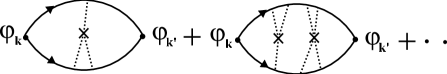
Figure 10: Impurity contributions to $\chi_{\mathrm{pp}}$ which are formally taken into account in our calculation.

Fig. 11 shows $n_{\mathrm{imp}}$ vs. $T_{\mathrm{c}}$ in the self-consistent 1-loop theory and, for comparison, that in the BCS model. In the self-consistent 1-loop theory, the critical impurity concentration for $t=0.2$ is larger than that for $t=0.3$ in spite of smaller $T_{\mathrm{c0}}$ for $t=0.2$ than for $t=0.3$. This situation is contrary to that in the BCS model without SC fluctuation. In $\S 2$, we have seen that $T_{\mathrm{c}}$ reduction in the BCS model almost coincides with AG curves and that $n_{\mathrm{imp}}^{\mathrm{c}}$ is given by $\frac{\pi^{2}\rho(0)T_{\mathrm{c0}}}{2\gamma^{\prime}}$ in AG formula, that is, $n_{\mathrm{imp}}^{\mathrm{c}}$ depends on $T_{\mathrm{c0}}$. Therefore, we can consider that the magnitude of $n_{\mathrm{imp}}^{\mathrm{c}}$ in the self-consistent 1-loop theory is mostly determined by the mean-field value of $n_{\mathrm{imp}}^{\mathrm{c}}$ which reflects the value of $T_{\mathrm{c0}}^{\mathrm{MF}}$. Strictly speaking, however, there exists the clear difference between $n_{\mathrm{imp}}^{\mathrm{c}}$ in the mean-field theory and that in the self-consistent 1-loop theory, as seen in Fig. 11. We consider that this difference originates from a quantum dynamics and will comment on this issue in $\S 4.4$.

Figure 11: $n_{\mathrm{imp}}$ vs. $T_{\mathrm{c}}$ in the BCS model and in the self-consistent 1-loop theory for the case of $t=0.2$ and $0.3$. The parameters are chosen as $g=0.4$ and $n=0.9$.

The most peculiar feature of $T_{\mathrm{c}}$ reduction is its nearly linear variation with impurity concentration. This is shown in Fig. 12 and 13. From Fig. 12, we can see that the curvature of $T_{\mathrm{c}}=T_{\mathrm{c}}(n_{\mathrm{imp}})$ gradually becomes positive as $t$ is small and the reduction of $T_{\mathrm{c}}$ is almost linear at $t=0.2$. This feature originates from the strong SC fluctuation. In Fig. 13, we compare the data for $t=0.2$ and AG curve. AG formula can not be the good fitting curve due to the absence of the negative curvature in the calculated data for $t=0.2$. Rullier-Albenque $et$ $al$. have reported this kind of the linear variation. [13] They have measured $T_{\mathrm{c}}$ and $ab$ plane resistivity of electron irradiated $\mathrm{YBa}_{\mathrm{2}}\mathrm{Cu}_{\mathrm{3}}\mathrm{O}_{\mathrm{7-\delta}}$ crystals (underdoped and optimally doped) and mensioned that the variation of $T_{\mathrm{c}}$ does not follow any current prediction of pair-beraking theories. However, we believe that a pair-breaking theory still holds even in their experiment and the ’pseudogap breaking’ by impurities or defects, which will be introduced below, is the reasonable keyword for an explanation of their data.

Figure 12: The $T_{\mathrm{c}}$ scaled by $T_{\mathrm{c0}}$ as the function of the impurity concentration. The parameters are chosen as $g=0.4$, $n=0.9$ and $t=0.1$, $0.2$ and $0.3$.

Figure 13: The $n_{\mathrm{imp}}$ vs. $T_{\mathrm{c}}$ data in the self-consistent 1-loop theory for the parameter as $t=0.2$, $g=0.4$, and $n=0.9$, and the fitting curve by Eq.(1). The fitting is done in the same way as in $\S 2$.

So, why the linear variation of $T_{\mathrm{c}}$ seen in Fig. 13 emerges?

Before tackling the issue, we analyze carefully Fig. 4.2 and Fig. 4.2 which show the spectral weight and the imaginary part of $\Sigma$ and $\Sigma_{\mathrm{sc}}$ at A and B in the $\mathbf{k}$-space as the funtion of $\omega$ for $n_{\mathrm{imp}}=0.00$, $0.07$, $0.14$. We proceed with a discussion regarding the point A as the representative of the $\mathbf{k}$-points around the ’hot spot’ and the point B as the one around the ’cold spot’, and then simply call A ’hot spot’ and B ’cold spot’ in the below discussion.

Comparing Fig. 4.2(a) and Fig. 4.2(a) for $n_{\mathrm{imp}}=0.00$, we find that the spectral weight at hot spot has a short peak but the one at cold spot has a sharp and high peak. This difference owes to the form factor $\varphi_{\mathbf{k}}^{2}$ which has a large value at hot spot and a small value at cold spot. Physically, it can be seen that because of SC fluctuation, there is almost no coherence as the well-defined quasi-particle at hot spot even in the clean case. Let us introduce impurities. We find the remarkable feature that whereas the spectral peak at cold spot is largely suppressed by impurities, the one at hot spot is hardly affected by impurities and keeps the almost same form as that in the clean case. Owing to the direct connection between the spectral weight and the imaginary part of the self-energy, this kind of feature also can be seen in Fig. 4.2(b) and Fig. 4.2(b) which show the quasi-particle damping, $|\mathrm{Im}\Sigma|$. As impurity concentration increases, while the lifetime of the quasi-particle at cold spot becomes short, the one at hot spot hardly changes. That is, impurities seem to mainly affect the quasi-particles at cold spot and have no contribution to the ones at hot spot, although the contribution of impurities to the quasi-particle damping should not depend on momentum $\mathbf{k}$. The reason that such things arise is clarified by taking accout of Fig. 4.2(c) and Fig. 4.2(c) which shows $\mathrm{Im}\Sigma_{\mathrm{sc}}$, the contribution of SC fluctuation to the quasi-particle damping. These figures have the common feature that $|\mathrm{Im}\Sigma_{\mathrm{sc}}|$ becomes small by impurities. It means that as impurities increase, the quasi-particles tend not to be affected by the SC fluctuation. In terms of our formulation, this is due to the diagram such as Fig. 14, which arises from the process of the self-consistent calculation. Impurities interfere in the scattering by the SC fluctuation. From these understandings, we can now appreciate the behavior that $|\mathrm{Im}\Sigma|$ at hot spot keeps the almost constant value at Fermi level. This is because the contribution of $\mathrm{Im}\Sigma_{\mathrm{sc}}$ cancels out the one of $\mathrm{Im}\Sigma_{\mathrm{imp}}$, and the cancellation makes $\mathrm{Im}\Sigma=\mathrm{Im}\Sigma_{\mathrm{sc}}+\mathrm{Im}\Sigma_{\mathrm{imp}}$ nearly constant. At cold spot, due to the smallness of the suppression of $|\mathrm{Im}\Sigma_{\mathrm{sc}}|$, the cancellation is not complete, and impurities effectively contribute there.

The idea of the suppression of $|\mathrm{Im}\Sigma_{\mathrm{sc}}|$ allows us to tackle the above issue. On the basis of the idea, we have drawn Fig. 15 which gives us a rough schematic understanding for the linear variation of $T_{\mathrm{c}}$. From the figure, the value of $T_{\mathrm{c}}$ in the self-consistent 1-loop theory can be expressed by the following form:

$$T_{\mathrm{c}}=T_{\mathrm{c}}^{\mathrm{MF}}-\delta T_{\mathrm{1}}-(\delta T_{\mathrm{imp}}-\delta T_{\mathrm{2}}),$$ (44)

where $\delta T_{\mathrm{imp}}$ $etc$. are explained in the caption of Fig. 15. As impurity concentration increases, not only $\delta T_{\mathrm{imp}}$ but also $\delta T_{\mathrm{2}}$ increases via the suppression of $|\mathrm{Im}\Sigma_{\mathrm{sc}}|$. Then, if $\delta T_{\mathrm{imp}}-\delta T_{\mathrm{2}}$ were in proportion to $n_{\mathrm{imp}}$, $T_{\mathrm{c}}$ would decrease linearly according as $n_{\mathrm{imp}}$ picks up. In this sense, our parameters used to draw Fig. 13 is such ones that keep the delicate balance between $\delta T_{\mathrm{2}}$ and $\delta T_{\mathrm{imp}}$ which leads to the nearly linear variation of $T_{\mathrm{c}}$ as the function of $n_{\mathrm{imp}}$. This is the answer for the above issue.

[t]

The spectral weight and the imaginary part of $\Sigma$ and $\Sigma_{\mathrm{sc}}$ as the function of real frequency $\omega$ obtained by the self-consistent 1-loop theory with impurities. Here, $t=0.2$, $g=0.4$, $T=0.02$, and $\mathbf{k}$ is at A in Fig. 7. The impurity concentrations $n_{\mathrm{imp}}$ are chosen as $n_{\mathrm{imp}}=0.00$, $0.07$ and $0.14$.

[t]

The spectral weight and the imaginary part of $\Sigma$ and $\Sigma_{\mathrm{sc}}$ as the function of real frequency $\omega$ obtained by the self-consistent 1-loop theory with impurities. Here, $t=0.2$, $g=0.4$, $T=0.02$, and $\mathbf{k}$ is at B in Fig. 7. The impurity concentrations $n_{\mathrm{imp}}$ are chosen as $n_{\mathrm{imp}}=0.00$, $0.07$ and $0.14$.

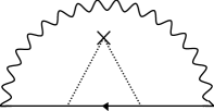
Figure 14: The example of the self-energy diagram included in the self-consistent calculation. The wavy line means SC fluctuation interaction and the dotted lines with the cross mark the impurities scattering averaged over on their positions. This type of diagram makes weak the contribution of SC fluctuation to the self-energy.

Figure 15: The figure for the rough understanding that $T_{\mathrm{c}}$ is suppressed almost linearly. $\delta T_{\mathrm{imp}}$ means the magnitude of the $T_{\mathrm{c}}$ reduction form $T_{\mathrm{c0}}^{\mathrm{MF}}$ in the BCS mean-field theory. $\delta T_{\mathrm{1}}$ means the difference of $T_{\mathrm{c0}}^{\mathrm{MF}}$ and $T_{\mathrm{c0}}$ in the self-consistent 1-loop theory, that is, the magnitude of suppression by SC fluctuation without impurities. The ’adjoint line’ is drawn by shifting the ’BCS($t=0.2$)’ data down by the amount of $\delta T_{\mathrm{1}}$. $\delta T_{\mathrm{2}}$ means the decline in the the magnitude of $T_{\mathrm{c}}$ reduction by SC fluctuation.

The essential and important point of the discussion up to here was the idea that $|\mathrm{Im}\Sigma_{\mathrm{sc}}|$ is suppressed by impurities. We call the idea ’psuedogap breaking’. We may doubt that the word is not consistent with the idea because there is no gap-like behavior in the spectral weight of Fig. 4.2 or Fig. 4.2. However, the pseudogap is indeed destructed by impurities as we will explain in $\S 4.3$.

Another important result we have to point out is included in Fig. 16 which shows the comparison of the quasi-particle damping by impurities in the self-consistent 1-loop theory and that in the mean-field theory. From the figure, we can see that the former is larger than the latter. As we mentioned in $\S 4.1$, SC fluctuation results in the reduced DOS. In our formulation, impurities are treated in the unitarity limit, then the reduced DOS leads to a large $\mathrm{Im}\Sigma_{\mathrm{imp}}$ as we can understand by Eq.(43). Therefore, the behavior shown in Fig. 16 can be interpleted by the reasoning that the contribution of impurities to the quasi-particle damping becomes effectively large by the effect of the SC fluctuation.

Figure 16: The impurities contribution to the imaginary part of self-energy as the function of $\omega$ in the self-consistent 1-loop theory(S1L) and in the mean-field theory(BCS). The parameters are chosen as $t=0.2$, $g=0.4$, $n=0.9$, and $T=0.02$.

4.3 Effective 1-loop model

In this section, we explain the concept of the ’pseudogap-breaking’ by impurities. To the aim, we introduce an effective model for the self-consistent 1-loop theory with impurities. The feature of this model is the maintenance of the gap-like behavior as can be seen in the 1-loop order theory even though the calculation to determine $T_{\mathrm{c}}$ is done self-consistently.

4.3.1 Derivation of the effective 1-loop model

Since $T(Q)$ has the sharp peak around $Q=(\mathbf{q},i\nu_{m})\cong 0$ for $T\cong T_{\mathrm{c}}$, we can expand $T(Q)^{-1}$ around $Q\cong 0$. Moreover, we use the static approximation, i.e. we only take into account $\nu_{m}=0$ for $T(\mathbf{q},i\nu_{m})$. Then

$$T(\mathbf{q},0)=\frac{-g}{1-g\chi_{\mathrm{pp}}(\mathbf{q},0)}$$ (45)

can be written as the following form:

$$T(\mathbf{q},0)\cong\frac{-g}{r+b\mathbf{q}^{2}},$$ (46)

where $b$ is a constant and

$$r=1-g\chi_{\mathrm{pp}}(\mathbf{0},0).$$ (47)

By making use of Eq.(46), we can rewrite Eq.(36) as follows:

$$\begin{split}&\Sigma_{\mathrm{sc}}(\mathbf{k},i\omega_{n})\\ &=\varphi_{\mathbf{k}}^{2}\frac{1}{\beta N}\sum_{\mathbf{q}}\frac{-g}{r+b\mathbf{q}^{2}}\frac{1}{-i\omega_{n}-\xi_{\mathbf{q-k}}-\Sigma_{\mathrm{imp}}(-i\omega_{n})}\\ &=\varphi_{\mathbf{k}}^{2}\frac{g}{\beta r\xi^{2}}\frac{1}{N}\sum_{\mathbf{q}}\frac{1}{\xi^{-2}+\mathbf{q}^{2}}\frac{1}{i\omega_{n}+\xi_{\mathbf{q-k}}+\Sigma_{\mathrm{imp}}(-i\omega_{n})}\\ &\cong\Delta^{2}\varphi_{\mathbf{k}}^{2}\frac{1}{N}\sum_{\mathbf{q}}\frac{2\xi^{-1}}{\xi^{-2}+q_{x}^{2}}\frac{2\xi^{-1}}{\xi^{-2}+q_{y}^{2}}\\ &\hskip 42.67912pt\times\frac{1}{i\omega_{n}+\xi_{\mathbf{k}}+v_{x}q_{x}+v_{y}q_{y}+\Sigma_{\mathrm{imp}}(-i\omega_{n})}.\end{split}$$ (48)

Here, $\xi^{2}\equiv b/r$, and we have replaced $\frac{1}{\xi^{2}+\mathbf{q}^{2}}$ with $\frac{\xi^{-1}}{\xi^{-2}+q_{x}^{2}}\frac{\xi^{-1}}{\xi^{-2}+q_{y}^{2}}$. Moreover, we have used that $\xi_{\mathbf{q-k}}$ around $\mathbf{q}\cong\mathbf{0}$ can be written as

$$\xi_{\mathbf{q-k}}=\xi_{\mathbf{k}}+v_{x}q_{x}+v_{y}q_{y},$$ (49)

where

$$v_{x}(\mathbf{k})=-2\sin k_{x}(t-2t^{\prime}\cos k_{y}),$$ (50)

and

$$v_{y}(\mathbf{k})=-2\sin k_{y}(t-2t^{\prime}\cos k_{x}),$$ (51)

and defined $\Delta^{2}$ as follows:

$$\Delta^{2}=-\frac{1}{\beta N}\sum_{\mathbf{q}}T(\mathbf{q},0).$$ (52)

By using this $\Delta^{2}$, we can express $\xi$ as

$$\xi=\sqrt{\frac{g}{4\beta r\Delta^{2}}}.$$ (53)

Integrating the last expression of Eq.(48), we finally obtain

$$\begin{split}&\Sigma_{\mathrm{sc}}(\mathbf{k},i\omega_{n})\\ &=\frac{\Delta^{2}\varphi_{\mathbf{k}}^{2}}{i\omega_{n}+\xi_{\mathbf{k}}+i(|v_{x}|+|v_{y}|)\xi^{-1}\mathrm{sgn}\omega_{n}+\Sigma_{\mathrm{imp}}(-i\omega_{n})}.\end{split}$$ (54)

The renormalized Green function is given by

$$G(\mathbf{k},i\omega_{n})=\frac{1}{i\omega_{n}-\xi_{\mathbf{k}}-\Sigma_{\mathrm{sc}}(\mathbf{k},i\omega_{n})-\Sigma_{\mathrm{imp}}(i\omega_{n})},$$ (55)

where $\Sigma_{\mathrm{imp}}(i\omega_{n})$ is as same as Eq.(43).

We solve Eqs.(38), (45), (52), (53), (54), (43) and (55) self-consistently choosing the chemical potential $\mu$ so as to keep $n=0.9$.

4.3.2 Results of calculation and ’pseudogap breaking’

Fig. 17 shows $t$-$T_{\mathrm{c}}$ phase diagram in the effective 1-loop model without impurities and for comparison that in the self-consistent 1-loop theory we have already displayed in Fig. 9. In the effective 1-loop theory, the larger suppression of $T_{\mathrm{c}}$ from the BCS value than that in the self-consistent 1-loop theory can be seen. That may be because we neglect the components of $\nu_{m}\neq 0$ in $T(\mathbf{q},i\nu_{m})$ and then the SC fluctuation as a thermal fluctuation is large in the effective model.

Fig. 18 shows $n_{\mathrm{imp}}$-$T_{\mathrm{c}}$ phase diagram in the effective 1-loop theory with the parameter is the same as in Fig. 11. The rough behavior of $T_{\mathrm{c}}$ is identical to that in the self-consistent 1-loop theory.

The obvious difference between the effective model and the self-consistent 1-loop theory is reflected in the spectral peak at hot spot which is shown in Fig. 4.3.2. The gap-like behavior in the spectral weight, that is, the pseudogap, can be seen in the data for $n_{\mathrm{imp}}=0.00$. It is notable that as $n_{\mathrm{imp}}$ increases, $|\mathrm{Im}\Sigma_{\mathrm{sc}}|$ becomes small, the pseudogap is suppressed, and then the single peak in the spectral weight emerges. This is nothing but ’pseudogap breaking’. Now, we have understood that the suppression of $|\mathrm{Im}\Sigma_{\mathrm{sc}}|$ by impurities is closely related to the pseudogap breaking.

Figure 17: $t$ vs. $T_{\mathrm{c}}$ in the self-consistent 1-loop theory and in the effective 1-loop model. The parameters are chosen as $g=0.4$ and $n=0.9$. The data of ’self-consistent 1-loop’ is as same as the data in Fig. 9.

Figure 18: $n_{\mathrm{imp}}$ vs. $T_{\mathrm{c}}$ in the effective 1-loop model for the case of $t=0.2$ and $0.3$. The parameters are chosen as $g=0.4$ and $n=0.9$.

[t]

The real and imaginary part of self-energy and the spectral weight as the function of $\omega$ obtained by the effective 1-loop theory with impurities. Here, $t=0.2$, $g=0.4$, $T=0.014$, and $\mathbf{k}$ is at A. The impurity concentrations $n_{\mathrm{imp}}$ are chosen as $n_{\mathrm{imp}}=0.00$, $0.05$, $0.10$, and $0.15$.

As is already mensioned, the suppression of $|\mathrm{Im}\Sigma_{\mathrm{sc}}|$ i.e. the pseudogap breaking, results from the self-energy diagram with such a form as Fig. 14. Because the causal relationship is very clear in the effective 1-loop theory, let us consider the relation again.

For simplicity, we adopt the following form of $\Sigma_{\mathrm{imp}}$,

$$\Sigma_{\mathrm{imp}}(i\omega_{n})=-i\frac{1}{2\tau}\mathrm{sgn}\omega_{n}.$$ (56)

Here, $\tau(\propto n_{\mathrm{imp}}^{-1})$ is the lifetime of the quasi-particle by impurity scttering. By using this expression, we can rewrite Eq.(54) as

$$\Sigma_{\mathrm{sc}}(\mathbf{k},i\omega_{n})=\frac{\Delta^{2}\varphi_{\mathbf{k}}^{2}}{i\omega_{n}+\xi_{\mathbf{k}}+i\Gamma_{\mathbf{k}}\mathrm{sgn}\omega_{n}},$$ (57)

where

$$\Gamma_{\mathbf{k}}=\frac{|v_{x}|+|v_{y}|}{\xi}+\frac{1}{2\tau}.$$ (58)

It is notable that the expression of Eq.(57) is nothing but the diagram of Fig. 14 itself within the approximation by which we have used to derive the effective 1-loop model. By analitical continuation, $i\omega_{n}\to\omega+i\delta$, in Eq.(57), we obtain

$$\mathrm{Im}\Sigma_{\mathrm{sc}}(\mathbf{k},\omega)=-\frac{\Delta^{2}\varphi_{\mathbf{k}}^{2}\Gamma_{\mathbf{k}}}{(\omega+\xi_{\mathbf{k}})^{2}+\Gamma_{\mathbf{k}}^{2}}.$$ (59)

From this equation, we find that $|\mathrm{Im}\Sigma_{\mathrm{sc}}(\mathbf{k},\omega)|$ has a peak at $\omega=0$ for the $\mathbf{k}$ on the Fermi surface and its top value is $\frac{\Delta^{2}\varphi_{\mathbf{k}}^{2}}{\Gamma_{\mathbf{k}}}$. Therefore, as $n_{\mathrm{imp}}$ increases, $\Gamma_{\mathbf{k}}$ becomes large, and then the peak of $|\mathrm{Im}\Sigma_{\mathrm{sc}}(\mathbf{k},\omega)|$ lowers. This tendency coincides with the behavior of $\mathrm{Im}\Sigma_{\mathrm{sc}}$ in Fig. 4.3.2. As the result, we recognize that the scattering process such as Fig. 14 is essential for pseudogap breaking. That is, the broadening of the one-particle state by impurities makes weak the scattering due to SC fluctuation and it leads to the pseudogap breaking.

4.4 Comments on the quantum dynamics of SC fluctuation

In $\S 4.2$, we have mensioned that the difference between $n_{\mathrm{imp}}^{\mathrm{c}}$ in the BCS theory and that in the self-consistent 1-loop theory. If the SC fluctuation were perfectly thermal, $n_{\mathrm{imp}}^{\mathrm{c}}$’s in the both theories would coincide with each other, because the thermal fluctuation should vanish at $T=0$. In the self-consistent 1-loop theory, however, the quantum dynamics of SC fluctuation is included. Actually, in Eq.(36), all $\nu_{m}$’s are included in the summation not just only $\nu_{m}=0$. Therefore, we expect that the above difference originates from the quantum dynamics. The expectation is supported by Fig. 19 which shows $n_{\mathrm{imp}}$ vs. $T_{\mathrm{c}}$ in some theories. The ’staticS1L’ in the figure means that we have applied the static approximation to Eq.(36), that is, taken just only $\nu_{m}=0$ into account in the self-consistent 1-loop theory. In Fig. 19, it can be seen that $n_{\mathrm{imp}}^{\mathrm{c}}$ in the three theories except the self-consistent 1-loop theory almost coincide with each other and $n_{\mathrm{imp}}^{\mathrm{c}}\sim 0.21$. The reason would be that in ’staticS1L’ and ’effective’, only the thermal fluctuation is taken into account. On the other hand, $n_{\mathrm{imp}}^{\mathrm{c}}$ in the self-consistent 1-loop theory is smaller than that in the other theories and $n_{\mathrm{imp}}^{\mathrm{c}}\sim 0.15$. Then, we consider that the quantum dynamics of SC fluctuation plays a role to reduce $n_{\mathrm{imp}}^{\mathrm{c}}$. Farther understanding about the quantum fluctuation is one of our future problems.

Figure 19: $n_{\mathrm{imp}}$ vs. $T_{\mathrm{c}}$ in the self-consistent 1-loop theory(S1L), S1L within the static approximation(staticS1L), the effective 1-loop model(effective) and the BCS mean-field theory(BCS). The parameters are chosen as $t=0.2$, $g=0.4$ and $n=0.9$ in all theories.

5 Conclusion

The reduction of $T_{\mathrm{c}}$ due to impurities in the FLEX theory is almost same as that in the weak-coupling $d$-wave BCS model. This is because the cancellation between two effects by impurities; one is the pair-weakening, and another is the reduction of the pair-breaking produced by electron correlation. Therefore, even in the HTS, where the pairing interaction is caused by $U$, AG formula still can be used for rough estimation of $T_{\mathrm{c}}$ reduction due to impurities. However, the following points should be noticed. By the numerical calculation, we have found the deviation of the critical impurity concentration from the $n_{\mathrm{imp}}^{\mathrm{c}}$ expected by AG formula. It depends on the fine structure of the dispersion and the Fermi surface via DOS. The larger is DOS, the larger the deviation of $n_{\mathrm{imp}}^{\mathrm{c}}$ is. In order to analyze the hole-doping dependence of $T_{\mathrm{c}}$ reduction by impurites in detail, we should notice the form of Fermi surface not just only adopting AG formula.

As for the dependence of impurity effect on $\mathbf{k}$-point, impurities mainly affect the quasi-particles at cold spot. This is because impurities reduce the inelastic scattering by spin fluctuation which is effective to the quasi-particles at hot spot. This is the good example to indicate that we ought to take into account the reduction of the damping rate of quasi-particle arising from electron interaction.

In $\S 4$, we have studied how pseudogap phenomena affect the reduction of $T_{\mathrm{c}}$ due to impurities. The variation of $T_{\mathrm{c}}$ as the function of $n_{\mathrm{imp}}$ is too linear to fit by AG formula in the region of rather large SC fluctuation. The linear variation is caused by the suppression of the quasi-particle damping arising from SC fluctuation i.e. the pseudogap breaking.

References

- [1] A. A. Abrikosov and L. P. Gor’kov, Sov. Phys. JETP (1961) 1243
- [2] T. Hotta, J. phys. Soc. Jpn. (1993) 274-280.
- [3] K. Ishida ., Physica C (1991) 29.
- [4] Y. Sun and K. Maki, Phys. Rev. B (1995) 6059.
- [5] N. E. Bickers, D. J. Scalapino, and S. R. White, Phys. Rev. Lett. (1989) 961.
- [6] N. E. Bickers and D. J. Scalapino, Ann. Phys. (N.Y.) (1989) 206.
- [7] C. H. Pao and N. E. Bickers, Phys. Rev. Lett. (1994) 1870.
- [8] P. Monthoux and D. J. Scalapino, Phys. Rev. Lett. (1994) 1874.
- [9] T. Dahm and L. Tewordt, Phys. Rev. B (1995) 1297.
- [10] A. Ino ., Phys. Rev. B (2002) 094504
- [11] T. Kluge ., Phys. Rev. B (1995) R727.
- [12] J. L. Tallon ., Phys. Rev. Lett. (1997) 5294.
- [13] F. Rullier-Albenque ., Phys.Rev. Lett. (2003) 047001
- [14] Y. Yanase and K. Yamada, J. Phys. Soc. Jpn. (1999) 2999.
- [15] Y. Yanase and K. Yamada, J. Phys. Soc. Jpn. (2000) 2209.
- [16] Y.Yanase ., Phys. Rep. (2004) 1.
- [17] B. Janko, J. Maly and K. Levin, Phys. Rev. B (1997) 11407.
- [18] J. Maly, B. Janko and K. Levin, Physica C (1999) 113.
- [19] D. Rohe and W. Metzner, Phys. Rev. B (2001) 224509.
- [20] Q.J. Chen and J.R. Schrieffer, Phys. Rev. B (2002) 014512.