Short-Time Decoherence for General System-Environment Interactions

Abstract

Short time approximation is developed for system-environmental bath mode interactions involving a general non-Hermitian system operator $\Lambda$, and its conjugate, $\Lambda^{\dagger}$, in order to evaluate onset of decoherence at low temperatures in quantum systems interacting with environment. The developed approach is complementary to Markovian approximations and appropriate for evaluation of quantum computing schemes. Example of a spin system coupled to a bosonic heat bath via $\Lambda\propto\sigma_{-}$ is worked out in detail.

I Introduction

Quantum system exposed to environmental modes is described by the reduced density matrix, and its evolution deviates from the ideal, usually pure-state, dynamics. For short times, appropriate for quantum computing gate functions and, generally, for controlled quantum dynamics, approximation schemes for the density matrix have been developed recently [Loss, -Onset2, ]. The present work derives a new rather general short-time approximation which applies for models with system-bath interactions involving a general system operator. It thus extends the previously known approach [Onset1, ,Onset2, ] which was limited to couplings involving a single Hermitian system operator.

We consider an open quantum system with the Hamiltonian

$$H=H_{S}+H_{B}+H_{I}.$$ (1)

Here $H_{S}$ describes the system proper. It is coupled to the environment (bath), described by $H_{B}$. The system and bath are coupled by the interaction $H_{I}$. The bath has been traditionally modelled [Loss, -Legg, ] by a large number of uncoupled bosonic modes, namely harmonic oscillators (with ground state energy shifted to zero),

$$H_{B}=\sum\limits_{k}\omega_{k}^{\vphantom{\dagger}}b_{k}^{\dagger}b_{k}^{\vphantom{\dagger}}.$$ (2)

Here $b_{k}$ are the bosonic annihilation operators corresponding to the bath modes, and from now on we use the convention $\hbar=1$.

In most of this work, we consider the general system $H_{S}$, and we assume that the interaction with the bath involves the system operator $\Lambda$ that couples linearly [VKam, -Grab, ] to the bath modes,

$$H_{I}=\Lambda\sum\limits_{k}g_{k}^{\vphantom{\dagger}}b_{k}^{\dagger}+\Lambda^{\dagger}\sum\limits_{k}g_{k}^{*}b_{k}^{\vphantom{\dagger}},$$ (3)

with the interaction constants $g_{k}$.

Let $R(t)$ denote the overall density matrix. It is commonly assumed [Loss, -Grab, ] that at time $t=0$ the system and bath are not entangled, and the bath modes are thermalized,

$$R\left(0\right)=\rho\left(0\right)\prod\limits_{k}\theta_{k},$$ (4)

where

$$\theta_{k}={\rm Z}_{k}^{-1}e^{-\beta\omega_{k}^{\vphantom{\dagger}}b_{k}^{\dagger}b_{k}^{\vphantom{\dagger}}},$$ (5)

with $\beta=1/kT$, and

$${\rm Z}_{k}\equiv\left(1-e^{-\beta\omega_{k}}\right)^{-1}.$$ (6)

We point out that while the quantum system $S$, described by the reduced density matrix $\rho(t)$, is small, typically two-state (qubit) or several-qubit, the bath has many degrees of freedom. The combined effect of the bath modes on the system can be large even if each of them is influenced little by the system. This has been the basis for the arguments for the harmonic approximation for the bath modes [Loss, -Legg, ] and the linearity of the interaction, as well as for the Markovian approximations [VKam, -Grab, ] that assume that the bath modes are “reset” to the thermal state by the “rest of the universe” on time scales shorter than any dynamical time of the system interacting with the bath.

The frequencies of the oscillators of the bath are usually assumed to be distributed from zero to some cutoff value $\omega_{c}$. The bath modes with the frequencies close to the energy gaps of the system, $\Delta E_{ij}=E_{i}-E_{j}$, contribute to the “resonant” thermalization and decoherence processes. Within the Markovian schemes, the diagonal elements of the reduced density matrix of the system,

$$\rho\left(t\right)=\mathrm{Tr}_{B}R\left(t\right),$$ (7)

approach the thermal values $\propto e^{-E_{i}/kT}$ for large times exponentially, on time scale $T_{1}$. The off-diagonal elements vanish, which represents decoherence, on time scale $T_{2}$, which, for resonant processes, is given by $T_{2}\simeq 2T_{1}$. However, generally decoherence is expected to be faster than thermalization because, in addition to resonant processes, it can involve virtual processes that do not conserve energy. It has been argued that this additional “pure” decoherence is dominated by the bath modes with near-zero frequencies [VKam, ,Grab, ,VKam2, ]. At low temperatures, this “pure decoherence” is expected [12, ] to make $T_{2}\ll T_{1}$.

Since the resetting of these low-frequency modes to the thermal state occurs on time scales $1/kT=\beta$, the Markovian approach cannot be used at low temperatures [VKam, ,Grab, ,VKam2, ]. Specifically, for quantum computing in solid-state semiconductor-heterostructure architectures [12, -22, ], temperatures as low as few $10$ mK are needed. This brings the thermal time scale to $\beta\sim 10^{-9}\,$sec, which is close to the single-qubit control times $10^{-11}\hbox{-}10^{-7}\,$sec [12, -22, ]. Alternatives to the Markovian approximation have been suggested [Ford, -Scnon, ].

In this work, we generalize the recently suggested scheme [Onset1, ,Onset2, ], applicable for Hermitian $\Lambda$ only, to a wider class of interaction Hamiltonians. We treat the case when the system operator $\Lambda$ entering the interaction, see (3), is not Hermitian. In actual applications in quantum computing, calculations with only a single qubit or few qubits are necessary for evaluation of the local “noise,” to use the criteria for quantum error correction [Shor, -Presk, ]. For example, the system Hamiltonian is frequently taken proportional to the Pauli matrix $\sigma_{z}$. The interaction operator $\Lambda$ can be proportional to $\sigma_{x}$, which is Hermitian. Such cases are covered by the short-time approximation developed earlier [Onset1, ,Onset2, ]. However, one can also consider models with $\Lambda\propto\sigma_{-}$. Similarly, models with non-Hermitian $\Lambda$ are encountered in Quantum Optics [Lois, ]. In Section II, we develop our short time approximation scheme. Results for a spin-boson type model are given in Section III.

II Short Time Approximation

In this section we obtain a general expression for the time evolution operator of the system (1-3) within the short time approximation. The system operators $H_{S}$ and $\Lambda$ need not be specified at this stage; the derivation is quite general.

In order to define “short time,” we consider dimensionless combinations involving the time variable $t$. There are several time scales in the problem. These include the inverse of the cutoff frequency of the bath modes, $1/{\omega_{c}}$, the thermal time $\beta=1/{kT}$, and the internal characteristic times of the system $1/{\Delta E_{ij}}$. Also, there are time scales associated with the system-bath interaction-generated thermalization and decoherence, $T_{1,2}$. The shortest time scale at low temperatures (when $\beta$ is large) is typically $1/{\omega_{c}}$. The most straightforward expansion in $t$ yields a series in powers of ${\omega_{c}}t$. The aim of developing more sophisticated short-time approximations [Onset1, ,Onset2, ] is to preserve unitarity and obtain expressions approximately valid up to intermediate times, of order of the system and interaction-generated time scales. The latter property can only be argued for heuristically in most cases, and checked by model calculations.

The overall density matrix, assuming time-independent Hamiltonian over the quantum-computation gate function time intervals [12, -22, ], evolves according to

$$R\left(t\right)=U(t)R\left(0\right)[U(t)]^{\dagger},$$ (8)

where

$$U(t)=e^{-i\left(H_{S}+H_{B}+H_{I}\right)t}$$ (9)

is the evolution operator.

The general idea of our approach is the following. We break the exponential operator in (9) into products of simpler exponentials. This involves an approximation, but allows us to replace system operators by their eigenvalues, when spectral representations are used, and then calculate the trace of $R(t)$ over the bath modes, obtaining explicit expressions for the elements of the reduced density matrix of the system. For Hermitian coupling operators, $\Lambda^{\dagger}=\Lambda$, our approach reduces to known results [Onset1, ,Onset2, ].

We split the exponential evolution operator into terms that do not have any noncommuting system operators in them. This requires an approximation. For short times, we start by using the factorization [Kirz, -Sorn, ]

$$e^{-i\left(H_{S}+H_{B}+H_{I}\right)t+O\left(t^{3}\right)}$$ (10)

$$= e^{-\frac{i}{2}H_{S}t}e^{-i\left(H_{I}+H_{B}\right)t}e^{-\frac{i}{2}H_{S}t},$$

where we have neglected terms of the third and higher orders in $t$, in the exponent. The middle exponential in (10),

$$\Xi\equiv e^{-i\left(H_{B}+H_{I}\right)t}=e^{-i\left(H_{B}+\Lambda G^{\dagger}+\Lambda^{\dagger}G\right)t},$$ (11)

where

$$G\equiv\sum\limits_{k}g_{k}^{*}b_{k},$$ (12)

still involves noncommuting terms as long as $\Lambda$ is non-Hermitian. In terms of the Hermitian operators

$$L\equiv{\frac{1}{2}}\left(\Lambda+\Lambda^{\dagger}\right),$$ (13)

$$M\equiv{\frac{i}{2}}\left(\Lambda-\Lambda^{\dagger}\right),$$ (14)

we have

$$\Lambda G^{\dagger}+\Lambda^{\dagger}G=L\left(G+G^{\dagger}\right)+iM\left(G-G^{\dagger}\right).$$ (15)

We then carry out two additional short-time factorizations within the same quadratic-in-$t$ (in the exponent) order of approximation,

$$\Xi = e^{\frac{1}{2}\left[M\left(G-G^{\dagger}\right)-iH_{B}\right]t}e^{\frac{i}{2}H_{B}t}$$

$$\times e^{-i\left[H_{B}+L\left(G+G^{\dagger}\right)\right]t}e^{\frac{i}{2}H_{B}t}e^{\frac{1}{2}\left[M\left(G-G^{\dagger}\right)-iH_{B}\right]t}.$$

This factorization is chosen in such a way that $\Xi$ remains unitary, and for $M=0$ or $L=0$ the expression is identical to that used for the Hermitian case [Onset1, ,Onset2, ]. The evolution operator then takes the form

$$U=e^{-\frac{i}{2}H_{S}t}\,\Xi\,e^{-\frac{i}{2}H_{S}t},$$ (17)

with $\Xi$ from (II), which is an approximation in terms of a product of several unitary operators.

It has been recognized [Onset1, ,Onset2, ] that approximations of this sort are superior to the straightforward expansion in powers of $t$ (or more exactly, $\omega_{c}t$). Specifically, in (10), we notice that $H_{S}$ is factored out in such a way that $H_{B}$, which commutes with $H_{S}$, droppes out of all the commutators that enter the higher-order correction terms. This suggests that a redefinition of the energies of the modes of $H_{B}$ should have only a limited effect on the corrections and serves as a heuristic argument for the approximation being valid beyond the shortest time scale $1/\omega_{c}$, up to intermediate time scales.

Our goal is to approximate the reduced density matrix of the system. We consider its energy-basis matrix elements,

$$\rho_{mn}\left(t\right)=\mathrm{Tr}_{B}\left\langle m\right|UR\left(0\right)U^{\dagger}\left|n\right\rangle,$$ (18)

where

$$H_{S}\left|n\right\rangle=E_{n}\left|n\right\rangle.$$ (19)

We next use the factorization (10,II) to systematically replace system operators by c-numbers, by inserting decompositions of the unit operator in the bases defined by $H_{S}$, $L$, and $M$. First, we collect the expressions (4,II,17, 19), and use two energy-basis decompositions of unity to get

$$\rho_{mn}\left(t\right) = \sum\limits_{p\,q}e^{\frac{i}{2}\left(E_{n}+E_{q}-E_{m}-E_{p}\right)t}\rho_{pq}\left(0\right)$$ (20)

$$\times \mathrm{Tr}_{B}\left[\left\langle m\right|\Xi\left|p\right\rangle\right.\prod\limits_{k}\theta_{k}\left.\left\langle q\right|\Xi^{\dagger}\left|n\right\rangle\right].$$

We now define the eigenstates of $L$ and $M$,

$$L\left|\lambda\right\rangle=\lambda\left|\lambda\right\rangle,$$ (21)

$$M\left|\mu\right\rangle=\mu\left|\mu\right\rangle.$$ (22)

The operators $\Xi$ and $\Xi^{\dagger}$ introduce exponentials in (20) that contain either $L$ or $M$ in the power. By appropriately inserting $\sum\limits_{\lambda}\left|\lambda\right\rangle\left\langle\lambda\right|$ or $\sum\limits_{\mu}\left|\mu\right\rangle\left\langle\mu\right|$ between these exponentials, we can convert all the remaining system operators to c-numbers. For convenience, let us define the operators

$$\pi_{\alpha\beta\gamma}=\left|\alpha\right\rangle\left\langle\alpha\right|\left.\beta\right\rangle\left\langle\beta\right.\left|\gamma\right\rangle\left\langle\gamma\right|\,\,\;\;\;\;\;$$ (23)

and

$${\cal U}_{s_{1},s_{2},s_{3}}=e^{s_{1}^{\vphantom{\dagger}}g_{k^{\vphantom{,}}}^{*}b_{k}^{\vphantom{\dagger}}t+s_{2}^{\vphantom{\dagger}}g_{k}^{\vphantom{\dagger}}b_{k}^{\dagger}t-is_{3}^{\vphantom{\dagger}}\omega_{k}^{\vphantom{\dagger}}b_{k}^{\dagger}b_{k}^{\vphantom{\dagger}}t}.$$ (24)

The resulting expression for the trace entering (20) is

$$\mathrm{Tr}_{B}\left\{\left\langle m\right|\Xi\left|p\right\rangle\right.\prod\limits_{k}\theta_{k}\left.\left\langle q\right|\Xi^{\dagger}\left|n\right\rangle\right\}$$ (25)

$$= \sum\limits_{\mu_{j}\lambda_{j}}\left\langle m\right|\pi_{\mu_{1}\lambda_{1}\mu_{2}}\left|p\right\rangle\left\langle q\right|\pi_{\mu_{3}\lambda_{2}\mu_{4}}\left|n\right\rangle\prod\limits_{k}{\cal T}_{k},$$

where the indices $\lambda$ and $\mu$ label the eigenstates of $L$ and $M$, respectively, and

$${{\cal T}_{k}} = \mathrm{Tr}_{k}\left\{{\cal U}_{\frac{1}{2}\mu_{1},-\frac{1}{2}\mu_{1},\frac{1}{2}}{\cal U}_{0,0,-\frac{1}{2}}{\cal U}_{-i\lambda_{1},-i\lambda_{1},1}\right.$$

$$\times {\cal U}_{0,0,-\frac{1}{2}}{\cal U}_{\frac{1}{2}\mu_{2},-\frac{1}{2}\mu_{2},\frac{1}{2}}\theta_{k}{\cal U}_{-\frac{1}{2}\mu_{3},\frac{1}{2}\mu_{3},-\frac{1}{2}}$$

$$\times \left.{\cal U}_{0,0,\frac{1}{2}}{\cal U}_{i\lambda_{2},i\lambda_{2},-1}{\cal U}_{0,0,\frac{1}{2}}{\cal U}_{-\frac{1}{2}\mu_{4},\frac{1}{2}\mu_{4},-\frac{1}{2}}\right\}.$$

In order to calculate the trace over the $k$th bath mode in (II), we rearrange the operators using the cyclic property, in such a way that the formula (52), derived in Appendix A, can be used to simplify products of two or three operators $\cal U$ at a time. For example, we can transfer the operator ${\cal U}_{\frac{1}{2}\mu_{1},-\frac{1}{2}\mu_{1},\frac{1}{2}}$ to the right hand side, getting the combination

$${\cal U}_{-\frac{1}{2}\mu_{4},\frac{1}{2}\mu_{4},-\frac{1}{2}}{\cal U}_{\frac{1}{2}\mu_{1},-\frac{1}{2}\mu_{1},\frac{1}{2}},$$ (27)

inside the trace, and use the identity (52). We then transfer ${\cal U}_{0,0,-\frac{1}{2}}$ to the right hand side and repeat the process, now for the three rightmost operators. After several steps we arrive to the following expression for the trace,

$${{\cal T}_{k}}={\cal R}_{k}\mathrm{Tr}_{k}\left\{\theta_{k}{\cal U}_{u,-u^{*},0}\right\},$$ (28)

where

$$u = \frac{i}{\omega_{k}t}\left(e^{-\frac{i\omega_{k}t}{2}}-1\right)\mu_{-}^{\prime\prime}-\frac{2i}{\omega_{k}t}e^{-\frac{i\omega_{k}t}{2}}\sin\frac{\omega_{k}t}{2}\lambda_{-}$$ (29)

$$+ \frac{i}{\omega_{k}t}e^{-\frac{i\omega_{k}t}{2}}\left(e^{-\frac{i\omega_{k}t}{2}}-1\right)\mu_{-}^{\prime}$$

and

$${\cal R}_{k}=\exp\Big{\{}\!\! - \!\frac{i\left|g_{k}\right|^{2}}{\omega_{k}^{2}}\Big{[}\big{(}\sin\frac{\omega_{k}t}{2}-\frac{\omega_{k}t}{2}\big{)}\left(\mu_{-}^{\prime}\mu_{+}^{\prime}+\mu_{-}^{\prime\prime}\mu_{+}^{\prime\prime}\right)+\left(\sin\omega_{k}t-\omega_{k}t\right)\lambda_{-}\lambda_{+}$$ (30)

$$- 4\sin\frac{\omega_{k}t}{2}\sin^{2}\frac{\omega_{k}t}{4}\mu_{-}^{\prime}\mu_{+}^{\prime\prime}-2\sin^{2}\frac{\omega_{k}t}{2}\left(\lambda_{-}\mu_{+}^{\prime\prime}-\lambda_{+}\mu_{-}^{\prime}\right)\Big{]}\Big{\}}.$$

Here we introduced the variables

$$\mu_{\pm}^{\prime} = \mu_{1}\pm\mu_{4},$$ (31)

$$\mu_{\pm}^{\prime\prime} = \mu_{2}\pm\mu_{3},$$ (32)

and

$$\lambda_{\pm}=\lambda_{1}\pm\lambda_{2}.$$ (33)

The trace in (28) can be evaluated, for instance, by using the coherent states technique, see Appendix B,

$${{\cal T}_{k}}={\cal R}_{k}e^{\frac{pq}{2}\left|g_{k}\right|^{2}t^{2}\coth\frac{\beta\omega_{k}}{2}}.$$ (34)

The expression which follows from (25), (29), (30) and (34) is

$$\prod\limits_{k}{{\cal T}_{k}}=\exp\left[-\mathcal{P}\left(t\right)\right],$$ (35)

where

$$\mathcal{P} = B^{2}\left(t\right)\left(\lambda_{-}^{2}+\mu_{-}^{\prime}\mu_{-}^{\prime\prime}\right)+B^{2}\left(t/2\right)\left(\mu_{-}^{\prime\prime}-\mu_{-}^{\prime}\right)^{2}-F\left(t\right)\left(\mu_{-}^{\prime\prime}-\mu_{-}^{\prime}\right)\lambda_{-}$$

$$- iC\left(t\right)\lambda_{-}\lambda_{+}-iC\left(t/2\right)\left(\mu_{-}^{\prime}\mu_{+}^{\prime}+\mu_{-}^{\prime\prime}\mu_{+}^{\prime\prime}\right)+iS\left(t\right)\left(\lambda_{-}\mu_{+}^{\prime\prime}-\lambda_{+}\mu_{-}^{\prime}\right)-iC_{1}\left(t\right)\mu_{-}^{\prime}\mu_{+}^{\prime\prime}.$$

The coefficients here are the spectral sums over the bath modes,

$$B^{2}\left(t\right)=2\sum\limits_{k}\frac{\left|g_{k}\right|^{2}}{\omega_{k}^{2}}\sin^{2}\frac{\omega_{k}t}{2}\coth\frac{\beta\omega_{k}}{2},$$ (37)

$$C\left(t\right)=\sum\limits_{k}\frac{\left|g_{k}\right|^{2}}{\omega_{k}^{2}}\left(\omega_{k}t-\sin\omega_{k}t\right);$$ (38)

these functions are well known [35, ,27, ]. The result also involves the new spectral functions

$$S\left(t\right)=-2\sum\limits_{k}\frac{\left|g_{k}\right|^{2}}{\omega_{k}^{2}}\sin^{2}\frac{\omega_{k}t}{2},$$ (39)

$$F\left(t\right)=4\sum\limits_{k}\frac{\left|g_{k}\right|^{2}}{\omega_{k}^{2}}\sin^{2}\frac{\omega_{k}t}{4}\sin\frac{\omega_{k}t}{2}\coth\frac{\beta\omega_{k}}{2}.$$ (40)

Furthermore, for the sake of convenience we defined

$$C_{1}\left(t\right)=2C\left(t/2\right)-C\left(t\right).$$ (41)

By using (20) and (35), we obtain our final result for the density matrix evolution,

$$\rho_{mn}\left(t\right) = \sum\limits_{p,q}\sum\limits_{\mu_{j}\lambda_{j}}e^{\frac{i}{2}\left(E_{n}+E_{q}-E_{m}-E_{p}\right)t}\rho_{pq}\left(0\right)$$

$$\times \left\langle m\right|\pi_{\mu_{1}\lambda_{1}\mu_{2}}\left|p\right\rangle\left\langle q\right|\pi_{\mu_{3}\lambda_{2}\mu_{4}}\left|n\right\rangle e^{-\mathcal{P}},$$

where the first sum over $p$ and $q$ is over the energy eigenstates of the system; the second sum is over $\lambda_{1},\lambda_{2}$ and $\mu_{1},\ldots,\mu_{4}$, which label the eigenstates of the operators $L$ and $M$, respectively; see (21) and (22).

III Discussion and Application

The result (II) looks formidable in the general case. However, in most applications evaluation of decoherence will require short-time expressions for the reduced density matrix of a single qubit. Few- and multi-qubit systems will have to be treated by utilizing additive quantities [norm, -addnorm, ], accounting for quantum error correction (requiring measurement), etc. For a two-state system—a qubit—the summation in (II) involves $2^{8}=64$ terms, each a product of several factors calculation of which is straightforward. Still, the required bookkeeping is cumbersome, and we utilized the symbolic language Mathematica to carry out the calculation for an illustrative example.

We consider the model [Swain, ] defined by

$$H=\mathcal{A}{\,}\sigma_{z}+\sum\limits_{k}\omega_{k}^{\vphantom{\dagger}}b_{k}^{\dagger}b_{k}^{\vphantom{\dagger}}+\sum\limits_{k}\left(g_{k}^{\vphantom{\dagger}}\sigma_{-}b_{k}^{\dagger}+g_{k}^{*}\sigma_{+}b_{k}^{\vphantom{\dagger}}\right),$$ (43)

where $\mathcal{A}\geq 0$ is a constant, $\sigma_{\pm}={1\over 2}(\sigma_{x}\pm\sigma_{y})$ and $\sigma_{z}$ are the Pauli matrices, $b_{k}^{\dagger}$ and $b_{k}^{\vphantom{\dagger}}$ are the bosonic creation and annihilation operators, and $g_{k}$ are the coupling constants. Physically this model may describe, for example, a qubit interacting with a bath of phonons, or a two-level molecule in an electromagnetic field. In the latter case, this is a variant of the multi-mode Jaynes-Cummings model [Lois, ,JC, ]. Certain spectral properties of this model, the field-theoretic counterpart of which is known as the Lee field theory, are known analytically, e.g., [Pf, ]. However, the trace over the bosonic modes, to obtain the reduced density matrix for the spin, has not been obtained exactly.

For the model (43) we have $\Lambda=\sigma_{-}$ and $\Lambda^{\dagger}=\sigma_{+}$, so that $L=\sigma_{x}/2$ and $M=\sigma_{y}/2.$ We have $\left|\lambda_{1,2}\right\rangle=\left(\left|\uparrow\right\rangle\pm\left|\downarrow\right\rangle\right)/\sqrt{2}$, with eigenvalues $\lambda_{1,2}=\pm 1/2$, and $\left|\mu_{1,2}\right\rangle=\left(\left|\uparrow\right\rangle\pm i\left|\downarrow\right\rangle\right)/\sqrt{2}$, with eigenvalues $\mu_{1,2}=\pm 1/2$. For the initial state, let us assume that the spin at $t=0$ is in the excited state $\left|\uparrow\right\rangle\left\langle\uparrow\right|$, so that the initial density matrix has the form

$$\rho\left(0\right)=\left(\begin{array}[]{cc}1&0\\ 0&0\end{array}\right).$$ (46)

Calculation in Mathematica yields the following results for the density matrix elements, $\rho_{12}(t)=0$ and

$$4\rho_{11}\left(t\right) = 2+\,e^{-2B^{2}\left(t\right)}+e^{-4B^{2}\left(\frac{t}{2}\right)}\cosh\left(2\,F\right)+2e^{-2B^{2}\left(\frac{t}{2}\right)}\sinh\left(B_{1}\right)\cos\left(S\right)$$

$$+ 2e^{-B^{2}\left(\frac{t}{2}\right)}\cos\left(C_{1}\right)\sin\left(S\right)+ie^{-B^{2}\left(t\right)-B^{2}\left(\frac{t}{2}\right)}\left[\,e^{iC_{1}}\sinh\left(-iS+F\right)+\,e^{-iC_{1}}\sinh\left(-iS-F\right)\right],$$

where $C_{1}$ was defined in (41) and

$$B_{1}(t)=2B^{2}\left(t/2\right)-B^{2}\left(t\right).$$ (48)

Where not explicitly shown, the argument of all the spectral functions entering (III) is $t$.

In order to obtain irreversible behavior and evaluate a measure of decoherence, we consider the continuum limit of infinitely many bath modes. We introduce the density of the bosonic bath states $\cal{D}\left(\omega\right)$, incorporating a large-frequency cutoff $\omega_{c}$, and replace the summations in (37)-(40) by integrations over $\omega$ [Legg, ,VKam, ,35, ,52, ]. For instance, (37) takes the form,

$$\ B^{2}\left(t\right)=\int\limits_{0}^{\infty}d\omega\frac{{\cal{D}}\left(\omega\right)|g(\omega)|^{2}}{\omega^{2}}\sin^{2}\frac{\omega t}{2}\coth\frac{\beta\omega}{2}.$$ (49)

We will use the standard Ohmic-dissipation [Legg, ] expression, with an exponential cutoff, for an illustrative calculation,

$${\cal{D}}\left(\omega\right)|g(\omega)|^{2}=\Omega\,\omega\,e^{-\omega/\omega_{c}},$$ (50)

where $\Omega$ is a constant.

We point out that the results obtained for the density matrix elements depend on the dimensionless variable $\omega_{c}t$, as well as on the dimensionless parameters $\Omega$ and $\omega_{c}\beta$ ($=\hbar\omega_{c}/kT$, where we remind the reader that $\hbar$, set to 1, must be restored in the final results). Interestingly, the results do not depend explicitly on the energy gap parameter $\mathcal{A}$, see (43). This illustrates the point that short-time approximations do not capture the “resonant” relaxation processes, but rather only account for “virtual” relaxation/decoherence processes dominated by the low-frequency bath modes. However, the short-time approximations of the type considered here are meaningful only for systems with well-defined separation of the resonant vs. virtual decoherence processes, i.e., for $\hbar/\mathcal{A}\gg 1/\omega_{c}$. For such systems, $\hbar/\mathcal{A}=1/\mathcal{A}$ defines one of the “intermediate” time scales beyond which the approximation cannot be trusted.

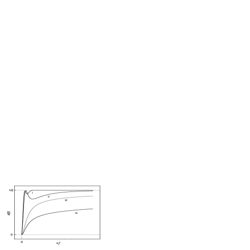
Figure 1: Schematic behavior of $s\left(t\right)$ for different values of $\Omega$, decreasing from $\sf{i}$ to $\sf{iv}$.

As an example, we calculated a measure of deviation of a qubit from a pure state in terms of the “linear entropy” [norm, ,addnorm, ,24, ],

$$s(t)=1-\mathrm{Tr}{\,}\left[\rho^{2}\left(t\right)\right].$$ (51)

Figure 1 schematically illustrates the behavior of $s(t)$ for different $\Omega$ values, for the case $\omega_{c}^{-1}<<\beta$. The values of $s(t)$ increase from zero, corresponding to a pure state, to $1/2$, corresponding to a completely mixed state, with superimposed oscillations. For Ohmic dissipation, three time regimes can be identified [27, ]. The shortest time scale is set by $t<O\left(1/{\omega_{c}}\right)$. The quantum-fluctuation dominated regime corresponds to $O\left(1/{\omega_{c}}\right)<t<O\left(1/{kT}\right)$. The thermal-fluctuation dominated regime is $t>O\left(1/{kT}\right)$. Our short time approximation yields reasonable results in the first two regimes. For $t>O\left(1/{kT}\right)$ it cannot correctly reproduce the process of thermalization. Instead, it predicts approach to the maximally mixed state.

Figure 2: The comparison between the $O(t^{2})$ expansion, $\sf{i}$, and the short-time approximation, $\sf{ii}$.

Figure 2 corresponds to the parameter values typical for low temperatures and appropriate for quantum computing applications, $\omega_{c}\beta=10^{3}$, with $\Omega=1.5\cdot 10^{-7}$ chosen to represent weak enough coupling to the bath to have the decoherence measure reach the threshold for fault-tolerance, of order $10^{-6}$, for “gate” times well exceeding $1/\omega_{c}$, here for $\omega_{c}t$ over 10. The leading-order quadratic expansion in powers of the time variable $t$ is also shown. Its validity is limited to $t<O\left(1/{\omega_{c}}\right)$ and it cannot be used for evaluation of quantum-computing models.

This research was supported by the National Security Agency and Advanced Research and Development Activity under Army Research Office contract DAAD-19-02-1-0035, and by the National Science Foundation, grant DMR-0121146.

Appendix A

Our aim is to derive a relation of the form

$${\cal U}_{v_{1},w_{1},x}{\cal U}_{v_{3},w_{3},0}{\cal U}_{v_{2},w_{2},-x}=\kappa{\cal U}_{p,q,0},$$ (52)

where the operator ${\cal U}_{s_{1},s_{2},s_{3}}$ was defined in (24). Consider the quantity

$$\Delta=e^{x\left(b^{\dagger}+\alpha_{1}\right)\left(b+\alpha_{2}\right)}e^{\gamma_{1}b^{\dagger}+\gamma_{2}b}e^{-x\left(b^{\dagger}+\beta_{1}\right)\left(b+\beta_{2}\right)},$$ (53)

where $b^{\dagger}$, $b$ are the bosonic creation and annihilation operators, $x$, $\alpha_{i}$, $\beta_{i}$ are c-numbers. Let us use the identity [Lois, ],

$$e^{\alpha b-\beta b^{\dagger}}f\left(b,b^{\dagger}\right)e^{-\alpha b+\beta b^{\dagger}}=f\left(b+\beta,b^{\dagger}+\alpha\right),$$ (54)

to represent the first and third exponentials in $\Delta$ in the form

$$e^{x\left(b^{\dagger}+\alpha_{1}\right)\left(b+\alpha_{2}\right)} = e^{\alpha_{1}b-\alpha_{2}b^{\dagger}}e^{xb^{\dagger}b}e^{-\alpha_{1}b+\alpha_{2}b^{\dagger}},$$ (55)

$$e^{-x\left(b^{\dagger}+\beta_{1}\right)\left(b+\beta_{2}\right)} = e^{\beta_{1}b-\beta_{2}b^{\dagger}}e^{-xb^{\dagger}b}e^{-\beta_{1}b+\beta_{2}b^{\dagger}}.$$ (56)

We then combine the second exponential in (53) and the last and first exponentials in (55) and (56), by utilizing the identity

$$e^{\alpha b}e^{\beta b^{\dagger}}=e^{\frac{1}{2}\alpha\beta}e^{\alpha b+\beta b^{\dagger}},$$ (57)

which follows from (54). The resulting exponential operator, with exponent linear in $b$ and $b^{\dagger}$, is sandwiched between $e^{xb^{\dagger}b}$ and $e^{-xb^{\dagger}b}$. Therefore, the following identity can be utilized [Lois, ],

$$e^{xb^{\dagger}b}f\left(b,b^{\dagger}\right)e^{-xb^{\dagger}b}=f\left(be^{-x},b^{\dagger}e^{x}\right).$$ (58)

Once again using (57), we arrive at the following expression,

$$\Delta=e^{\nu b+\mu b^{\dagger}+r},$$ (59)

where

$$\mu=\left(\alpha_{2}-\beta_{2}\right)\left(e^{x}-1\right)+\gamma_{1}e^{x},$$ (60)

$$\nu=\left(\beta_{1}-\alpha_{1}\right)\left(e^{-x}-1\right)+\gamma_{2}e^{-x},$$ (61)

and

$$r = -2\left(\alpha_{1}\beta_{2}-\alpha_{2}\beta_{1}\right)\sinh^{2}\frac{x}{2}+\left(\alpha_{1}\alpha_{2}-\beta_{1}\beta_{2}\right)\sinh x$$ (62)

$$+ \frac{1}{2}\gamma_{1}\left(\alpha_{1}+\beta_{1}\right)\left(e^{x}-1\right)+\frac{1}{2}\gamma_{2}\left(\alpha_{2}+\beta_{2}\right)\left(e^{-x}-1\right).$$

Now (52) follows, with

$$\kappa = \exp\left[\frac{2\left|g_{k}\right|^{2}}{x^{2}\omega_{k}^{2}}\sin^{2}\left(\frac{x\omega_{k}t}{2}\right)\left(v_{1}w_{2}-v_{2}w_{1}\right)\right]$$ (63)

$$\times \exp\left[\frac{i\left|g_{k}\right|^{2}}{x^{2}\omega_{k}^{2}}\left(\sin\left(x\omega_{k}t\right)\left(v_{1}w_{1}-v_{2}w_{2}\right)+x\omega_{k}t\left(v_{2}w_{2}-v_{1}w_{1}\right)\right)\right]$$

$$\times \exp\left[\frac{i\left|g_{k}\right|^{2}t}{2x\omega_{k}}\left(\left(e^{-ix\omega_{k}t}-1\right)w_{3}\left(v_{1}-v_{2}\right)+\left(e^{ix\omega_{k}t}-1\right)v_{3}\left(w_{1}-w_{2}\right)\right)\right],$$

and

$$p=-\frac{i}{x\omega_{k}t}\left(e^{ix\omega_{k}t}-1\right)\left(v_{1}+v_{2}\right)+v_{3}e^{ix\omega_{k}t}\,\,\,\,\,\,,$$ (64)

$$q=\frac{i}{x\omega_{k}t}\left(e^{-ix\omega_{k}t}-1\right)\left(w_{1}+w_{2}\right)+w_{3}e^{-ix\omega_{k}t}.$$ (65)

Appendix B

Let us calculate the trace in (28) which has the form

$${\cal T}\equiv\mathrm{Tr}\left\{e^{\delta b^{\dagger}b}e^{vb+wb^{\dagger}}\right\},$$ (66)

where we omitted the index $k$ since all the calculations here are in the space of a single mode. We use the coherent-state technique [Lois, ]. The coherent states $\left|z\right\rangle$ by definition are eigenstates of the annihilation operator, $b$

$$b\left|z\right\rangle=z\left|z\right\rangle,$$ (67)

with complex eigenvalues $z=x+iy$. These states are not orthogonal

$$\left\langle z_{1}\right|\left.z_{2}\right\rangle=\exp\left(z_{1}^{*}z_{2}-\frac{1}{2}\left|z_{1}\right|^{2}-\frac{1}{2}\left|z_{2}\right|^{2}\right),$$ (68)

and they form an overcomplete set. The identity operator can be written as

$$\int d^{2}z\left|z\right\rangle\left\langle z\right|=1,$$ (69)

where the integration in complex plane is defined via

$$d^{2}z=\frac{1}{\pi}dxdy.$$ (70)

We represent the trace (66) by the coherent-state integral using the relation

$$\mathrm{Tr}A=\int d^{2}z\left\langle z\right|A\left|z\right\rangle,$$ (71)

where $A$ is an arbitrary operator. We then use the normal ordering, $\mathcal{N}$, formula for bosonic operators, represented schematically (see [Lois, ] for details) by

$$e^{\delta b^{\dagger}b}=\mathcal{N}e^{b^{\dagger}\left(e^{\delta}-1\right)b}.$$ (72)

The second term in the trace in (66) is split by using (57). All instances of $b$ and $b^{\dagger}$ can then be replaced by $z$ and $z^{*}$, and the integral evaluated to yield the expression for the trace,

$${\cal T}=\frac{e^{\frac{wv}{2}\coth\frac{\delta}{2}}}{1-e^{\delta}}.$$ (73)

References

• (1) D. Loss and D. P. DiVincenzo, Exact Born Approximation for the Spin-Boson Model, e-print cond-mat/0304118 at www.arxiv.org.
• (2) V. Privman, J. Stat. Phys. 110, 957 (2003).
• (3) V. Privman, Mod. Phys. Lett. B 16, 459 (2002).
• (4) R. P. Feynman and A. R. Hibbs, Quantum Mechanics and Path Integrals (McGraw-Hill, NY, 1965).
• (5) G. W. Ford, M. Kac and P. Mazur, J. Math. Phys. 6, 504 (1965).
• (6) A. O. Caldeira and A. J. Leggett, Phys. Rev. Lett. 46, 211 (1981).
• (7) A. O. Caldeira and A. J. Leggett, Physica A 121, 587 (1983).
• (8) S. Chakravarty and A. J. Leggett, Phys. Rev. Lett. 52, 5 (1984).
• (9) A. J. Leggett, S. Chakravarty, A. T. Dorsey, M. P. A. Fisher and W. Zwerger, Rev. Mod. Phys. 59, 1 (1987) [Erratum ibid. 67, 725 (1995)].
• (10) N. G. van Kampen, Stochastic Processes in Physics and Chemistry (North-Holland, Amsterdam, 2001).
• (11) W. H. Louisell, Quantum Statistical Properties of Radiation (Wiley, NY, 1973).
• (12) A. Abragam, The Principles of Nuclear Magnetism (Clarendon Press, Oxford, 1983).
• (13) K. Blum, Density Matrix Theory and Applications (Plenum, NY, 1996).
• (14) H. Grabert, P. Schramm and G.-L. Ingold, Phys. Rep. 168, 115 (1988).
• (15) N. G. van Kampen, J. Stat. Phys. 78, 299 (1995).
• (16) V. Privman, D. Mozyrsky and I. D. Vagner, Computer Phys. Commun. 146, 331 (2002).
• (17) D. Loss and D. P. DiVincenzo, Phys. Rev. A 57, 120 (1998).
• (18) V. Privman, I. D. Vagner and G. Kventsel, Phys. Lett. A 239, 141 (1998).
• (19) B. E. Kane, Nature 393, 133 (1998).
• (20) A. Imamoglu, D. D. Awschalom, G. Burkard, D. P. DiVincenzo, D. Loss, M. Sherwin and A. Small, Phys. Rev. Lett. 83, 4204 (1999).
• (21) R. Vrijen, E. Yablonovitch, K. Wang, H. W. Jiang, A. Balandin, V. Roychowdhury, T. Mor and D. P. DiVincenzo, Phys. Rev. A 62, 012306 (2000).
• (22) S. Bandyopadhyay, Phys. Rev. B 61, 13813 (2000).
• (23) D. Mozyrsky, V. Privman and M. L. Glasser, Phys. Rev. Lett. 86, 5112 (2001).
• (24) G. W.Ford and R. F. O’Connell, J. Optics B 5, 349 (2003).
• (25) K. M. Fonseca Romero, S.Kohler and P.Hänggi, Chem. Phys. 296, 307 (2004).
• (26) K. M. Fonseca Romero, P. Talkner and P. Hänggi, Is the Dynamics of Open Quantum Systems Always Linear?, e-print quant-ph/0311077 at www.arxiv.org.
• (27) R. F. O’Connell, Physica E 19, 77 (2003).
• (28) Y. Makhlin and A. Shnirman, Dephasing of Solid-State Qubits at Optimal Points, e-print cond-mat/0308297 at www.arxiv.org.
• (29) Y. Makhlin, G. Schön and A. Shnirman, Dissipation in Josephson Qubits, e-print cond-mat/0309049 at www.arxiv.org.
• (30) P. W. Shor, in Proc. 37th Ann. Symp. Found. Comp. Sci. (IEEE Comp. Sci. Soc. Press, Los Alamitos, CA, 1996), p. 56.
• (31) D. Aharonov and M. Ben-Or, Fault-Tolerant Quantum Computation with Constant Error, e-prints quant-ph/9611025 and quant-ph/9906129 at www.arxiv.org.
• (32) A. Steane, Phys. Rev. Lett. 78, 2252 (1997).
• (33) E. Knill and R. Laflamme, Phys. Rev. A 55, 900 (1997).
• (34) D. Gottesman, Phys. Rev. A 57, 127 (1998).
• (35) J. Preskill, Proc. Royal Soc. London A 454, 385 (1998).
• (36) D. A. Kirzhnits, Field Theoretical Methods in Many-Body Systems (Pergamon Press, Oxford, 1967).
• (37) M. Suzuki and K. Umeno, in Computer Simulation Studies in Condensed-Matter Physics VI (Springer Proc. Phys., Vol. 76), ed. D. P. Landau, K. K. Mon and H.-B. Sch ttler (Springer-Verlag, Berlin, 1993), p. 55.
• (38) A. T. Sornborger and E. D. Stewart, Phys. Rev. A 60, 1956 (1999).
• (39) G. M. Palma, K. A. Suominen and A. K. Ekert, Proc. Royal Soc. London A 452, 567 (1996).
• (40) D. Mozyrsky and V. Privman, J. Stat. Phys. 91, 787 (1998).
• (41) L. Fedichkin, A. Fedorov and V. Privman, Proc. SPIE 5105, 243 (2003).
• (42) L. Fedichkin and A. Fedorov, Decoherence Rate of Semiconductor Charge Qubit Coupled to Acoustic Phonon Reservoir, e-print quant-ph/0309024 at www.arxiv.org.
• (43) L. Fedichkin, A. Fedorov and V. Privman, Additivity of Decoherence Measures for Multiqubit Quantum Systems, e-print cond-mat/0309685 at www.arxiv.org.
• (44) S. Swain, J. Phys. A 5, 1587 (1972).
• (45) E. T. Jaynes and F. W. Cummings, Proc. IEEE 51, 89 (1963).
• (46) P. Pfeifer, Phys. Rev. A 26, 701 (1982).
• (47) D. Mozyrsky and V. Privman, Modern Phys. Lett. B 14, 303 (2000).
• (48) W. H. Zurek, S. Habib and J. P. Paz, Phys. Rev. Lett. 70, 1187 (1993).