Time-dependent density-matrix renormalization-group using adaptive effective Hilbert spaces

Abstract

An algorithm for the simulation of the evolution of slightly entangled quantum states has been recently proposed as a tool to study time-dependent phenomena in one-dimensional quantum systems. Its key feature is a time-evolving block-decimation (TEBD) procedure to identify and dynamically update the relevant, conveniently small subregion of the otherwise exponentially large Hilbert space. Potential applications of the TEBD algorithm are the simulation of time-dependent Hamiltonians, transport in quantum systems far from equilibrium and dissipative quantum mechanics. In this paper we translate the TEBD algorithm into the language of matrix product states in order to both highlight and exploit its resemblances to the widely used density-matrix renormalization-group (DMRG) algorithms. The TEBD algorithm, being based on updating a matrix product state in time, is very accessible to the DMRG community and it can be enhanced by using well-known DMRG techniques, for instance in the event of good quantum numbers. More importantly, we show how it can be simply incorporated into existing DMRG implementations to produce a remarkably effective and versatile “adaptive time-dependent DMRG” variant, that we also test and compare to previous proposals.

1 Introduction

Over many decades the description of the physical properties of low-dimensional strongly correlated quantum systems has been one of the major tasks in theoretical condensed matter physics. Generically, this task is complicated by the strong quantum fluctuations present in such systems which are usually modelled by minimal-model Hubbard or Heisenberg-style Hamiltonians. Despite the apparent simplicity of these Hamiltonians, few analytically exact solutions are available and most analytical approximations remain uncontrolled. Hence, numerical approaches have always been of particular interest, among them exact diagonalization and quantum Monte Carlo.

Decisive progress in the description of the low-energy equilibrium properties of one-dimensional strongly correlated quantum Hamiltonians was achieved by the invention of the density-matrix renormalization-group (DMRG) [1, 2]. It is concerned with the iterative decimation of the Hilbert space of a growing quantum system such that some quantum state, say the ground state, is approximated in that restricted space with a maximum of overlap with the true state. Let the quantum state of a one-dimensional system be

$$|\psi\rangle=\sum_{i}\sum_{j}\psi_{ij}|i\rangle|j\rangle,$$ (1)

where we consider a partition of the system into two blocks S and E, and where $\{|i\rangle\}$ and $\{|j\rangle\}$ are orthonormal bases of S and E respectively. Then the DMRG decimation procedure consists of projecting $|\psi\rangle$ on the Hilbert spaces for S and E spanned by the $M$ eigenvectors $|w_{\alpha}^{S}\rangle$ and $|w_{\alpha}^{E}\rangle$ corresponding to the largest eigenvalues $\lambda_{\alpha}^{2}$ of the reduced density matrices

$$\hat{\rho}_{S}={\rm Tr}_{E}|\psi\rangle\langle\psi|\quad\quad\hat{\rho}_{E}={\rm Tr}_{S}|\psi\rangle\langle\psi|,$$ (2)

such that $\hat{\rho}_{S}|w_{\alpha}^{S}\rangle=\lambda_{\alpha}^{2}|w_{\alpha}^{S}\rangle$ and $\hat{\rho}_{E}|w_{\alpha}^{E}\rangle=\lambda_{\alpha}^{2}|w_{\alpha}^{E}\rangle$. That both density matrices have the same eigenvalue spectrum is reflected in the guaranteed existence of the so-called Schmidt decomposition of the wave function [3],

$$|\psi\rangle=\sum_{\alpha}\lambda_{\alpha}|w_{\alpha}^{S}\rangle|w_{\alpha}^{E}\rangle,\quad\lambda_{\alpha}\geq 0,$$ (3)

where the number of positive $\lambda_{\alpha}$ is bounded by the dimension of the smaller of the bases of S and E.

Recently [4, 5, 6, 7, 8, 9], the ability of the DMRG decimation procedure to preserve the entanglement of $|\psi\rangle$ between S and E has been studied in the context of quantum information science [3, 10]. This blooming field of research, bridging between quantum physics, computer science and information theory, offers a novel conceptual framework for the study of quantum many-body systems [3, 4, 5, 6, 7, 8, 9, 10, 11, 12, 13, 14, 15, 16, 17]. New insights into old quantum many-body problems can be gained from the perspective of quantum information science, mainly through its eagerness to characterize quantum correlations. As an example, a better understanding of the reasons of the breakdown of the DMRG in two-dimensional systems has been obtained in terms of the growth of bipartite entanglement in such systems [7, 9].

More specifically, in quantum information the entanglement of $|\psi\rangle$ between S and E is quantified by the von Neumann entropy of $\hat{\rho}_{S}$ (equivalently, of $\hat{\rho}_{E}$),

$$\mathcal{S}(\hat{\rho}_{S})=-\sum\lambda_{\alpha}^{2}\log_{2}\lambda_{\alpha}^{2},$$ (4)

a quantity that imposes a useful (information theoretical) bound $M\geq 2^{\mathcal{S}}$ on the minimal number $M$ of states to be kept during the DMRG decimation process if the truncated state is to be similar to $|\psi\rangle$. On the other hand, arguments from field theory imply that, at zero temperature, strongly correlated quantum systems are in some sense only slightly entangled in $d=1$ dimensions but significantly more entangled in $d>1$ dimensions: In particular, in $d=1$ a block corresponding to $l$ sites of a gapped infinite-length chain has an entropy $\mathcal{S}_{l}$ that stays finite even in the thermodynamical limit $l\rightarrow\infty$, while at criticality $\mathcal{S}_{l}$ only grows logarithmically with $l$. It is this saturation or, at most, moderate growth of $\mathcal{S}_{l}$ that ultimately accounts for the succeess of DMRG in $d=1$. Instead, in the general $d$-dimensional case the entropy of bipartite entanglement for a block of linear dimension $l$ scales as $\mathcal{S}_{l}\sim l^{d-1}$. Thus, in $d=2$ dimensions the DMRG algorithm should keep a number $M$ of states that grows exponentially with $l$, and the simulation becomes inefficient for large $l$ (while still feasible for small $l$).

While DMRG has yielded an enormous wealth of information on the static and dynamic equilibrium properties of one-dimensional systems[18, 19] and is arguably the most powerful method in the field, only few attempts have been made so far to determine the time evolution of the states of such systems, notably in a seminal paper by Cazalilla and Marston [20]. This question is of relevance in the context of the time-dependent Hamiltonians realized e.g. in cold atoms in optical lattices [21, 22], in systems far from equilibrium in quantum transport, or in dissipative quantum mechanics. However, in another example of how quantum information science can contribute to the study of quantum many-body physics, one of us (G.V.) has recently developed an algorithm for the simulation of slightly entangled quantum computations [23] that can be used to simulate time evolutions of one-dimensional systems [17].

This new algorithm, henceforth referred to as the time-evolving block decimation (TEBD) algorithm, considers a small, dynamically updated subspace of the blocks S and E in Eq. (3) to efficiently represent the state of the system, as we will review in detail below. It was originally developed in order to show that a large amount of entanglement is necessary in quantum computations, the rationale there being quite simple: any quantum evolution (e.g. a quantum computation) involving only a “sufficiently restricted” amount of entanglement can be efficiently simulated in a classical computer using the TEBD algorithm; therefore, from an algorithmical point of view, any such quantum evolution is not more powerful than a classical computation.

Regardless of the implications for computer science, the above connection between the amount of entanglement and the complexity of simulating quantum systems is of obvious practical interest in condensed matter physics since, for instance, in $d=1$ dimensions the entanglement of most quantum systems happens to be “sufficiently restricted” precisely in the sense required for the TEBD algorithm to yield an efficient simulation. In particular, the algorithm has already been implemented and tested successfully on spin chains[17], the Bose-Hubbard model and single-atom transistors[24] and dissipative systems at finite temperature [25].

A primary aim of this paper is to reexpress the TEBD algorithm in a language more familiar to the DMRG community than the one originally used in Refs. [17, 23], which made substantial use of the quantum information parlance. This turns out to be a rewarding task since, as we show, the conceptual and formal similarities between the TEBD and DMRG are extensive. Both algorithms search for an approximation to the true wave function within a restricted class of wave functions, which can be identified as matrix product states [26], and had also been previously proposed under the name of finitely-correlated states[27]. Arguably, the big advantage of the TEBD algorithm relies on its flexibility to flow in time through the submanifold of matrix product states. Instead of considering time evolutions within some restricted subspace according to a fixed, projected, effective Hamiltonian, the TEBD algorithm updates a matrix product state in time using the bare Hamiltonian directly. Thus, in a sense, it is the Schrödinger equation that decides, at each time step, which are the relevant eigenvectors for S and E in Eq. (3), as opposed to having to select them from some relatively small, pre-selected subspace.

A second goal of this paper is to show how the two algorithms can be integrated. The TEBD algorithm can be improved by considering well-known DMRG techniques, such as the handling of good quantum numbers. But most importantly, we will describe how the TEBD simulation algorithm can be incorporated into preexisting, quite widely used DMRG implementations, the so-called finite-system algorithm[2] using White’s prediction algorithm[28]. The net result is an extremely powerful “adaptive time-dependent DMRG” algorithm, that we test and compare against previous proposals.

The outline of this paper is as follows: In Section 2, we discuss the problems currently encountered in applying DMRG to the calculation of explicitly time-dependent quantum states. Section 3 reviews the common language of matrix product states. We then express both the TEBD simulation algorithm (Sec. 4) and DMRG (Sec. 5) in this language, revealing where both methods coincide, where they differ and how they can be combined. In Section 6, we then formulate the modifications to introduce the TEBD algorithm into standard DMRG to obtain the adaptive time-dependent DMRG, and Section 7 discusses an example application, concerning the quantum phase transition between a superfluid and a Mott-insulating state in a Bose-Hubbard model. To conclude, we discuss in Section 8 the potential of the new DMRG variant.

2 Simulation of time-dependent quantum phenomena using DMRG

The first attempt to simulate the time evolution of quantum states using DMRG is due to Cazalilla and Marston [20]. After applying a standard DMRG calculation using the Hamiltonian $\hat{H}(t=0)$ to obtain the ground state of the system at $t=0$, $|\psi_{0}\rangle$, the time-dependent Schrödinger equation is numerically integrated forward in time, building an effective $\hat{H}_{{\rm eff}}(t)=\hat{H}_{{\rm eff}}(0)+\hat{V}_{{\rm eff}}(t)$, where $\hat{H}_{{\rm eff}}(0)$ is taken as the Hamiltonian approximating $\hat{H}(0)$ in the truncated Hilbert space generated by DMRG. $\hat{V}_{{\rm eff}}(t)$ as an approximation to $\hat{V}(t)$ is built using the representations of operators in the block bases obtained in the standard DMRG calculation of the $t=0$ state. $\hat{V}(t)$ contains the changes in the Hamiltonian with respect to the starting Hamiltonian: $\hat{H}(t)=\hat{H}_{0}+\hat{V}(t)$. The (effective) time-dependent Schrödinger equation reads

$$i\frac{\partial}{\partial t}|\psi(t)\rangle=[\hat{H}_{{\rm eff}}-E_{0}+\hat{V}_{{\rm eff}}(t)]|\psi(t)\rangle,$$ (5)

where the time-dependence of the ground state resulting of $\hat{H}(0)$ has been transformed away. If the evolution of the ground state is looked for, the initial condition is obviously to take $|\psi(0)\rangle=|\psi_{0}\rangle$ obtained by the preliminary DMRG run. Forward integration can be carried out by step-size adaptive methods such as the Runge-Kutta integration based on the infinitesimal time evolution operator

$$|\psi(t+\delta t)\rangle=(1-{\rm i}\hat{H}(t)\delta t)|\psi(t)\rangle,$$ (6)

where we drop the subscript denoting that we are dealing with effective Hamiltonians only. The algorithm used was a fourth-order adaptive size Runge-Kutta algorithm [29].

Sources of errors in this approach are twofold, due to the approximations involved in numerically carrying out the time evolution, and to the fact that all operators live on a truncated Hilbert space.

For the systems studied we have obtained a conceptually simple improvement concerning the time evolution by replacing the explicitly non-unitary time-evolution of Eq. (6) by the unitary Crank-Nicholson time evolution

$$|\psi(t+\delta t)\rangle=\frac{1-{\rm i}\hat{H}(t)\delta t/2}{1+{\rm i}\hat{H}(t)\delta t/2}|\psi(t)\rangle.$$ (7)

To implement the Crank-Nicholson time evolution efficiently we have used a (non-Hermitian) biconjugate gradient method to calculate the denominator of Eq. (7). In fact, this modification ensures higher precision of correlators, and the occurence of asymmetries with respect to reflection in the results decreased.

It should be noted, however, that for the Crank-Nicholson approach only lowest-order expansions of the time evolution operator $\exp(-{\rm i}\hat{H}\delta t)$ have been taken; we have not pursued feasible higher-order expansions.

As a testbed for time-dependent DMRG methods we use throughout this paper the time-dependent Bose-Hubbard Hamiltonian,

$$\hat{H}_{BH}(t)=-J\sum_{i=1}^{L-1}b^{\dagger}_{i+1}b^{\phantom{\dagger}}_{i}+b^{\dagger}_{i}b^{\phantom{\dagger}}_{i+1}+\frac{U(t)}{2}\sum_{i=1}^{L}n_{i}(n_{i}-1),$$ (8)

where the (repulsive) onsite interaction $U>0$ is taken to be time-dependent. This model exhibits for commensurate filling a Kosterlitz-Thouless-like quantum phase transition from a superfluid phase for $u<u_{c}$ (with $u=U/J$) to a Mott-insulating phase for $u>u_{c}$. We have studied a Bose-Hubbard model with $L=8$ and open boundary conditions, total particle number $N=8$, $J=1$, and instantaneous switching from $U_{1}=2$ in the superfluid phase to $U_{2}=40$ in the Mott phase at $t=0$. We consider the nearest-neighbor correlation, a robust numerical quantity, between sites 2 and 3. Up to 8 bosons per site (i.e. $N_{{\rm site}}=9$ states per site) were allowed to avoid cut-off effects in the bosonic occupation number in all calculations in this Section. All times in this paper are measured in units of $\hbar/J$ or $1/J$, setting $\hbar\equiv 1$. Comparing Runge-Kutta and Crank-Nicholson (with time steps of $\delta t=5\times 10^{-5}$) we found the latter to be numerically preferable; all static time-dependent DMRG calculations have been carried out using the latter approach.

However, Hilbert space truncation is at the origin of more severe approximations. The key assumption underlying the approach of Cazalilla and Marston is that the effective static Hilbert space created in the preliminary DMRG run is sufficiently large that $|\psi(t)\rangle$ can be well approximated within that Hilbert space for all times, such that

$$\epsilon(t)=1-|\langle\psi(t)|\psi_{{\rm exact}}(t)\rangle|$$ (9)

remains small as $t$ grows. This, in general, will only be true for relatively short times. A variety of modifications that should extend the reach of the static Hilbert space in time can be imagined. They typically rest on the DMRG practice of “targeting” several states: to construct the reduced density matrix used to determine the relevant Hilbert space states, one may carry out a partial trace over a mixture of a small number of states such that the truncated Hilbert space is constructed so that all of those states are optimally approximated in the DMRG sense:

$$\hat{\rho}_{S}={\rm Tr}_{E}|\psi\rangle\langle\psi|\rightarrow\hat{\rho}_{S}={\rm Tr}_{E}\sum_{i}\alpha_{i}|\psi_{i}\rangle\langle\psi_{i}|.$$ (10)

A simple choice uses the targeting of $\hat{H}^{n}|\psi_{0}\rangle$, for $n$ less than 10 or so, approximating the short-time evolution, which we have found to substantially improve the quality of results for non-adiabatic switching of Hamiltonian parameters in time: convergence in $M$ is faster and more consistent with the new DMRG method (see below).

Similarly, we have found that for adiabatic changes of Hamiltonian parameters results improve if one targets the ground states of both the initial and final Hamiltonian. These approaches are conceptually very similar to targeting not only $|\psi_{0}\rangle$, but also $\hat{O}|\psi_{0}\rangle$ and some $\hat{H}^{n}\hat{O}|\psi_{0}\rangle$, $n=1,2,3,\ldots$ in Lanczos vector dynamics DMRG[30, 31], or real and imaginary part of $(\hat{H}-\omega-E_{0}+{\rm i}\eta)^{-1}\hat{O}|\psi_{0}\rangle$ in correction vector dynamics DMRG[31, 32] to calculate Green’s functions

$$\langle\psi_{0}|\hat{O}^{\dagger}\frac{1}{H-\omega-E_{0}+{\rm i}\eta}\hat{O}|\psi_{0}\rangle.$$ (11)

To illustrate the previous approaches, we show results for the parameters of the Bose-Hubbard model discussed above. Time evolution is calculated in the Crank-Nicholson approach using a stepwidth $\delta t=5\cdot 10^{-5}$ in time units of $\hbar/J$ targeting (i) just the superfluid ground state $|\psi_{0}\rangle$ for $U_{1}=2$ (Fig. 1), (ii) in addition to (i) also the Mott-insulating ground state $|\psi_{0}^{\prime}\rangle$ for $U_{2}=40$ and $\hat{H}(t>0)|\psi_{0}\rangle$ (Fig. 2), (iii) in addition to (i) and (ii) also $\hat{H}(t>0)^{2}|\psi_{0}\rangle$ and $\hat{H}(t>0)^{3}|\psi_{0}\rangle$ (Fig. 3).

We have used up to $M=200$ states to obtain converged results (meaning that we could observe no difference between the results for $M=100$ and $M=200$) for $t\leq 4$, corresponding to roughly 25 oscillations. The results for the cases (ii) and (iii) are almost converged for $M=50$, whereas (i) shows still crude deviations.

Figure 1: Time evolution of the real part of the nearest-neighbor correlations in a Bose-Hubard model with instantaneous change of interaction strength at $t=0$: superfluid state targeting only. The different curves for different $M$ are shifted.

Figure 2: Time evolution of the real part of the nearest-neighbor correlations in a Bose-Hubard model with instantaneous change of interaction strength at $t=0$: targeting of the initial superfluid ground state, Mott insulating ground state and one time-evolution step. The different curves for different $M$ are shifted.

Figure 3: Time evolution of the real part of the nearest-neighbor correlations in a Bose-Hubard model with instantaneous change of interaction strength at $t=0$: targeting of the initial superfluid ground state, Mott insulating ground state and three time-evolution steps. The different curves for different $M$ are shifted.

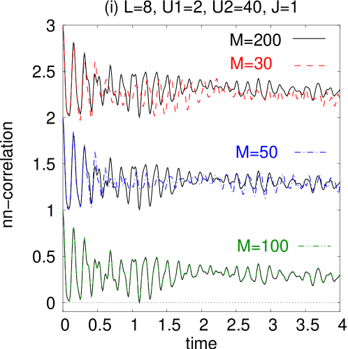
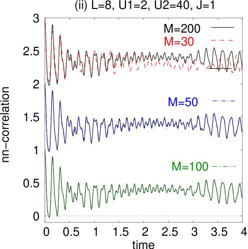
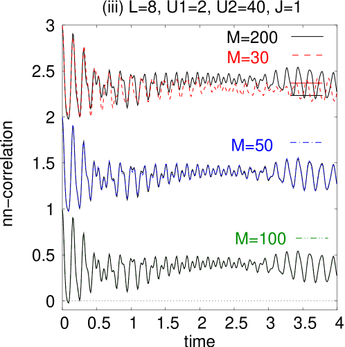
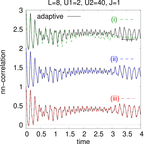
A remarkable observation can be made if one compares the three $M=200$ curves (Fig. 4), which by standard DMRG procedure (and for lack of a better criterion) would be considered the final, converged outcome, both amongst each other or to the result of the new adaptive time-dependent DMRG algorithm which we are going to discuss below: result (i) is clearly not quantitatively correct beyond very short times, whereas result (ii) agrees very well with the new algorithm, and result (iii) agrees almost (beside some small deviations at $t\approx 3$) with result (ii) and the new algorithm. Therefore we see that for case (i) the criterion of convergence in $M$ does not give a good control to determine if the obtained results are correct. This raises as well doubts about the reliability of this criterion for cases (ii) and (iii).

Figure 4: Comparison of the three $M=200$ Crank-Nicholson calculations to adaptive time-dependent DMRG at $M=50$: we target (i) just the superfluid ground state $|\psi_{0}\rangle$ for $U_{1}=2$ (Fig. 1), (ii) in addition to (i) also the Mott-insulating ground state $|\psi_{0}^{\prime}\rangle$ for $U_{2}=40$ and $\hat{H}(t>0)|\psi_{0}\rangle$ (Fig. 2), (iii) in addition to (i) and (ii) also $\hat{H}(t>0)^{2}|\psi_{0}\rangle$ and $\hat{H}(t>0)^{3}|\psi_{0}\rangle$. The different curves are shifted.

A more elaborate, but also much more time-consuming improvement still within the framework of a static Hilbert space was proposed by Luo, Xiang and Wang [33, 34]. Additional to the ground state they target a finite number of quantum states at various discrete times using a bootstrap procedure starting from the time evolution of smaller systems that are iteratively grown to the desired final size.

The observation that even relatively robust numerical quantities such as nearest-neighbor correlations can be qualitatively and quantitatively improved by the additional targeting of states which merely share some fundamental characteristics with the true quantum state (as we will never reach the Mott-insulating ground state) or characterize only the very short-term time evolution indicates that it would be highly desirable to have a modified DMRG algorithm which, for each time $t$, selects Hilbert spaces of dimension $M$ such that $|\psi(t)\rangle$ is represented optimally in the DMRG sense, thus attaining at all times the typical DMRG precision for $M$ retained states. The presentation of such an algorithm is the purpose of the following sections.

3 Matrix product states

As both the TEBD simulation algorithm and DMRG can be neatly expressed in the language of matrix product states, let us briefly review the properties of these states also known as finitely-correlated states[27, 26].

We begin by considering a one-dimensional system of size $L$, divided up into sites which each have a local Hilbert space, $\mathcal{H}_{i}$. For simplicity we take the same dimension $N_{{\rm site}}$ at all sites. In such a system a product state may be expressed as

$$|\mbox{\boldmath$\sigma$\unboldmath}\rangle=|\sigma_{1}\rangle\otimes|\sigma_{2}\rangle\otimes\ldots\otimes|\sigma_{L}\rangle,$$ (12)

where $|\sigma_{i}\rangle$ denotes the local state on site $i$. We can express a general state of the whole system as

$$|\psi\rangle = \sum_{\sigma_{1},\ldots,\sigma_{L}}\psi_{\sigma_{1},\ldots,\sigma_{L}}|\sigma_{1}\rangle\otimes|\sigma_{2}\rangle\otimes\ldots\otimes|\sigma_{L}\rangle$$ (13)

$$\equiv \sum_{\mbox{\boldmath$\sigma$\unboldmath}}\psi_{\mbox{\boldmath$\sigma$\unboldmath}}|\mbox{\boldmath$\sigma$\unboldmath}\rangle.$$

This general state exists in the Hilbert space $\mathcal{H}=\prod_{i=1}^{L}\mathcal{H}_{i}$, with dimension $(N_{{\rm site}})^{L}$.

A matrix product state is now formed by only using a specific set of expansion coefficients $\psi_{\mbox{\boldmath$\sigma$\unboldmath}}$. Let us construct this set in the following. To do this we define operators $\hat{A}_{i}[\sigma_{i}]$ which correspond to a local basis state $|\sigma_{i}\rangle$ at site $i$ of the original system, but which act on auxiliary spaces of dimension $M$, i.e.,

$$\hat{A}_{i}[\sigma_{i}]=\sum_{\alpha,\beta}A^{i}_{\alpha\beta}[\sigma_{i}]|\alpha\rangle\langle\beta|,$$ (14)

where $|\alpha\rangle$ and $|\beta\rangle$ are orthonormal basis states in auxiliary spaces. For visualization, we imagine the auxiliary state spaces to be located on the bonds next to site $i$. If we label the bond linking sites $i$ and $i+1$ by $i$, then we say that the states $|\beta\rangle$ live on bond $i$ and the states $|\alpha\rangle$ on bond $i-1$. The operators $\hat{A}_{i}[\sigma_{i}]$ hence act as transfer operators past site $i$ depending on the local state on site $i$. On the first and last site, which will need special attention later, this picture involves bonds $0$ and $L$ to the left of site 1 and to the right of site $L$ respectively. While these bonds have no physical meaning for open boundary conditions, they are identical and link sites 1 and $L$ as one physical bond for periodic boundary conditions. There is no a priori significance to be attached to the states in the auxiliary state spaces.

In general, operators corresponding to different sites can be different. If this is the case the resulting matrix product state to be introduced is referred to as a position dependent matrix product state. We also impose the condition

$$\sum_{\sigma_{i}}\hat{A}_{i}[\sigma_{i}]\hat{A}_{i}^{\dagger}[\sigma_{i}]=\mathcal{I},$$ (15)

which we will see to be related to orthonormality properties of bases later. An unnormalized matrix product state in a form that will be found useful for Hamiltonians with open boundary conditions is now defined as

$$|\tilde{\psi}\rangle=\sum_{\mbox{\boldmath$\sigma$\unboldmath}}\left(\langle\phi_{L}|\prod_{i=1}^{L}\hat{A}_{i}[\sigma_{i}]|\phi_{R}\rangle\right)|\mbox{\boldmath$\sigma$\unboldmath}\rangle,$$ (16)

where $|\phi_{L}\rangle$ and $|\phi_{R}\rangle$ are the left and right boundary states in the auxiliary spaces on bonds 0 and $L$. They act on the product of the operators $\hat{A}_{i}$ to produce scalar coefficients

$$\psi_{\mbox{\boldmath$\sigma$\unboldmath}}=\langle\phi_{L}|\prod_{i=1}^{L}\hat{A}_{i}[\sigma_{i}]|\phi_{R}\rangle$$ (17)

for the expansion of $|\tilde{\psi}\rangle$.

Several remarks are in order. It should be emphasized that the set of states obeying Eq. (16) is an (arbitrarily constructed) submanifold of the full boundary-condition independent Hilbert space of the quantum many-body problem on $L$ sites that is hoped to yield good approximations to the true quantum states for Hamiltonians with open boundary conditions. If the dimension $M$ of the auxiliary spaces is made sufficiently large then any general state of the system can, in principle, be represented exactly in this form (provided that $|\phi_{L}\rangle$ and $|\phi_{R}\rangle$ are chosen appropriately), simply because the $O(N_{{\rm site}}LM^{2})$ degrees of freedom to choose the expansion coefficients will exceed $N_{{\rm site}}^{L}$. This is, of course, purely academic. The practical relevance of the matrix product states even for computationally manageable values of $M$ is shown by the success of DMRG, which is known[35, 36] to produce matrix product states of auxiliary state space dimension $M$, in determining energies and correlators at very high precision for moderate values of $M$. In fact, some very important quantum states in one dimension, such as the valence-bond-solid (VBS) ground state of the Affleck-Kennedy-Lieb-Tasaki (AKLT) model [37, 38, 39], can be described exactly by matrix product states using very small $M$ ($M=2$ for the AKLT model).

Let us now formulate a Schmidt decomposition for matrix product states which can be done very easily. An unnormalized state $|\tilde{\psi}\rangle$ of the matrix-product form of Eq. (16) with auxiliary space dimension $M$ can be written as

$$|\tilde{\psi}\rangle=\sum_{\alpha=1}^{M}|\tilde{w}^{S}_{\alpha}\rangle|\tilde{w}^{E}_{\alpha}\rangle,$$ (18)

where we have arbitrarily cut the chain into S on the left and E on the right with

$$|\tilde{w}^{S}_{\alpha}\rangle=\sum_{\{\mbox{\boldmath$\sigma$\unboldmath}^{S}\}}\left[\langle\phi_{L}|\prod_{i\in S}\hat{A}_{i}[\sigma_{i}]|\alpha\rangle\right]|\mbox{\boldmath$\sigma$\unboldmath}^{S}\rangle,$$ (19)

and similarly $|\tilde{w}^{E}_{\alpha}\rangle$, where $\{|\alpha\rangle\}$ are the states spanning the auxiliary state space on the cut bond. Normalizing the states $|\tilde{\psi}\rangle$, $|\tilde{w}^{S}_{\alpha}\rangle$ and $|\tilde{w}^{E}_{\alpha}\rangle$ we obtain the representation

$$|\psi\rangle=\sum_{\alpha=1}^{M}\lambda_{\alpha}|w^{S}_{\alpha}\rangle|w^{E}_{\alpha}\rangle$$ (20)

where in $\lambda_{\alpha}$ the factors resulting from the normalization are absorbed. The relationship to reduced density matrices is as detailed in Sec. 1.

4 TEBD Simulation Algorithm

Let us now express the TEBD simulation algorithm in the language of the previous section. In the original exposition of the algorithm [23], one starts from a representation of a quantum state where the coefficients for the states are decomposed as a product of tensors,

$$\psi_{\sigma_{1},\ldots,\sigma_{L}}=\sum_{\alpha_{1},\ldots,\alpha_{L-1}}\Gamma^{[1]\sigma_{1}}_{\alpha_{1}}\lambda^{[1]}_{\alpha_{1}}\Gamma^{[2]\sigma_{2}}_{\alpha_{1}\alpha_{2}}\lambda^{[2]}_{\alpha_{2}}\Gamma^{[3]\sigma_{3}}_{\alpha_{2}\alpha_{3}}\cdots\Gamma^{[L]\sigma_{L}}_{\alpha_{L-1}}.$$ (21)

It is of no immediate concern to us how the $\Gamma$ and $\lambda$ tensors are constructed explicitly for a given physical situation. Let us assume that they have been determined such that they approximate the true wave function close to the optimum obtainable within the class of wave functions having such coefficients; this is indeed possible as will be discussed below. There are, in fact, two ways of doing it, within the framework of DMRG (see below), or by a continuous imaginary time evolution from some simple product state, as discussed in Ref. [17].

Let us once again attempt a visualization; the (diagonal) tensors $\lambda^{[i]}$, $i=1,\ldots,L-1$ are associated with the bonds $i$, whereas $\Gamma^{[i]}$, $i=2,\ldots,L-1$ links (transfers) from bond $i$ to bond $i-1$ across site $i$. Note that at the boundaries ($i=1,L$) the structure of the $\Gamma$ is different, a point of importance in the following. The sums run over $M$ states $|\alpha_{i}\rangle$ living in auxiliary state spaces on bond $i$. A priori, these states have no physical meaning here.

Figure 5: Bipartitioning by cutting bond $l$ between sites $l$ and $l+1$.

The $\Gamma$ and $\lambda$ tensors are constructed such that for an arbitrary cut of the system into a part $S_{l}$ of length $l$ and a part $E_{L-l}$ of length $L-l$ at bond $l$, the Schmidt decomposition for this bipartite splitting reads

$$|\psi\rangle=\sum_{\alpha_{l}}\lambda^{[l]}_{\alpha_{l}}|w_{\alpha_{l}}^{S_{l}}\rangle|w_{\alpha_{l}}^{E_{L-l}}\rangle,$$ (22)

with

$$|w_{\alpha_{l}}^{S_{l}}\rangle=\sum_{\alpha_{1},\ldots,\alpha_{l-1}}\sum_{\sigma_{1},\ldots,\sigma_{l}}\Gamma^{[1]\sigma_{1}}_{\alpha_{1}}\lambda^{[1]}_{\alpha_{1}}\cdots\Gamma^{[l]\sigma_{l}}_{\alpha_{l-1}\alpha_{l}}|\sigma_{1}\rangle\otimes\cdots\otimes|\sigma_{l}\rangle,$$ (23)

and

$$|w_{\alpha_{l}}^{E_{L-l}}\rangle = \sum_{\alpha_{l},\ldots,\alpha_{L-1}}\sum_{\sigma_{l+1},\ldots,\sigma_{L}}\Gamma^{[l+1]\sigma_{l+1}}_{\alpha_{l}\alpha_{l+1}}\lambda^{[l+1]}_{\alpha_{l+1}}\cdots\Gamma^{[L]\sigma_{L}}_{\alpha_{L-1}}\times$$ (24)

$$|\sigma_{l+1}\rangle\otimes\cdots\otimes|\sigma_{L}\rangle,$$

where $|\psi\rangle$ is normalized and the sets of $\{|w_{\alpha_{l}}^{S_{l}}\rangle\}$ and $\{|w_{\alpha_{l}}^{E_{L-l}}\rangle\}$ are orthonormal. This implies, for example, that

$$\sum_{\alpha_{l}}(\lambda_{\alpha_{l}}^{[l]})^{2}=1.$$ (25)

We can see that (leaving aside normalization considerations for the moment) this representation may be expressed as a matrix product state if we choose for $\hat{A}_{i}[\sigma_{i}]=\sum_{\alpha,\beta}A^{i}_{\alpha\beta}[\sigma_{i}]|\alpha\rangle\langle\beta|$

$$A^{i}_{\alpha\beta}[\sigma_{i}]=\Gamma^{[i]\sigma_{i}}_{\alpha\beta}\lambda^{[i]}_{\beta},$$ (26)

except for $i=1$, where we choose

$$A^{1}_{\alpha\beta}[\sigma_{1}]=f_{\alpha}\Gamma^{[1]\sigma_{1}}_{\beta}\lambda^{[1]}_{\beta},$$ (27)

and for $i=L$, where we choose

$$A^{L}_{\alpha\beta}[\sigma_{L}]=\Gamma^{[L]\sigma_{L}}_{\alpha}g_{\beta}.$$ (28)

The vectors $f_{\alpha}$ and $g_{\beta}$ are normalised vectors which must be chosen in conjunction with the boundary states $|\phi_{L}\rangle$ and $|\phi_{R}\rangle$ so as to produce the expansion (21) from this choice of the $\hat{A}_{i}$. Specifically, we require

$$|\phi_{L}\rangle = \sum_{\alpha}f_{\alpha}|\alpha\rangle$$ (29)

$$|\phi_{R}\rangle = \sum_{\beta}g^{*}_{\beta}|\beta\rangle,$$ (30)

where $|\alpha\rangle$ and $|\beta\rangle$ are the states forming the same orthonormal basis in the auxiliary spaces on bonds 0 and $L$ used to express $A^{i}_{\alpha\beta}$. In typical implementations of the algorithm it is common to take $f_{\alpha}=g_{\alpha}=\delta_{\alpha,1}$. Throughout the rest of the article we take this as the definition for $g_{\alpha}$ and $f_{\alpha}$, as this allows us to treat the operators on the boundary identically to the other operators for the purposes of the simulation protocol. For the same reason we define a vector $\lambda^{[0]}_{\alpha}=\delta_{\alpha,1}$.

In the above expression we have grouped $\Gamma$ and $\lambda$ such that the $\lambda$ reside on the right of the two bonds linked by $\Gamma$. There is another valid choice for the $\hat{A}_{i}$, which will produce identical states in the original system, and essentially the same procedure for the algorithm. If we set

$$\tilde{A}^{i}_{\alpha\beta}[\sigma_{i}]=\lambda^{[i-1]}_{\alpha}\Gamma^{[i]\sigma_{i}}_{\alpha\beta},$$ (31)

except for $i=1$, where we choose

$$\tilde{A}^{1}_{\alpha\beta}[\sigma_{1}]=f_{\alpha}\Gamma^{[1]\sigma_{1}}_{\beta},$$ (32)

and for $i=L$, where we choose

$$\tilde{A}^{L}_{\alpha\beta}[\sigma_{L}]=\lambda^{[L-1]}_{\alpha}\Gamma^{[L]\sigma_{L}}_{\alpha}g_{\beta},$$ (33)

then the same choice of boundary states produces the correct coefficients. Here we have grouped $\Gamma$ and $\lambda$ such that the $\lambda$ reside on the left of the two bonds linked by $\Gamma$. It is also important to note that any valid choice of $f_{\alpha}$ and $g_{\beta}$ that produces the expansion (21) specifically excludes the use of periodic boundary conditions. While generalizations are feasible, they lead to a much more complicated formulation of the TEBD simulation algorithm and will not be pursued here.

To conclude the identification of states, let us consider normalization issues. The condition (15) is indeed fulfilled for our choice of $A_{i}[\sigma_{i}]$, because we have from (24) for a splitting at $l$ that

$$|w_{\alpha_{l-1}}^{E_{L-(l-1)}}\rangle = \sum_{\alpha_{l}\sigma_{l}}\Gamma^{[l]\sigma_{l}}_{\alpha_{l-1}\alpha_{l}}\lambda^{[l]}_{\alpha_{l}}|\sigma_{l}\rangle\otimes|w_{\alpha_{l}}^{E_{L-l}}\rangle$$ (34)

$$= \sum_{\alpha_{l}\sigma_{l}}A^{l}_{\alpha_{l-1}\alpha_{l}}[\sigma_{l}]|\sigma_{l}\rangle\otimes|w_{\alpha_{l}}^{E_{L-l}}\rangle,$$

so that from the orthonormality of the sets of states $\{|w_{\alpha}^{E_{L-(l-1)}}\rangle\}_{\alpha=1}^{M}$, $\{|\sigma_{l}\rangle\}_{\sigma_{l}=1}^{N_{{\rm site}}}$ and $\{|w_{\gamma}^{E_{L-l}}\rangle\}_{\gamma=1}^{M}$,

$$\sum_{\sigma_{l}}\hat{A}_{l}[\sigma_{l}]\hat{A}^{\dagger}_{l}[\sigma_{l}] = \sum_{\alpha\beta\gamma}\sum_{\sigma_{l}}A^{l}_{\alpha\gamma}[\sigma_{l}](A^{l}_{\beta\gamma}[\sigma_{l}])^{*}|\alpha\rangle\langle\beta|$$ (35)

$$= \sum_{\alpha\beta}\langle w_{\beta}^{E_{L-(l-1)}}|w_{\alpha}^{E_{L-(l-1)}}\rangle|\alpha\rangle\langle\beta|$$

$$= \sum_{\alpha\beta}\delta_{\alpha\beta}|\alpha\rangle\langle\beta|=\mathcal{I}.$$

Let us now consider the time evolution for a typical (possibly time-dependent) Hamiltonian in strongly correlated systems that contains only short-ranged interactions, for simplicity only nearest-neighbor interactions here:

$$\hat{H}=\sum_{i\>\rm odd}\hat{F}_{i,i+1}+\sum_{j\rm\>even}\hat{G}_{j,j+1},$$ (36)

$F_{i,i+1}$ and $G_{j,j+1}$ are the local Hamiltonians on the odd bonds linking $i$ and $i+1$, and the even bonds linking $j$ and $j+1$. While all $F$ and $G$ terms commute among each other, $F$ and $G$ terms do in general not commute if they share one site. Then the time evolution operator may be approximately represented by a (first order) Trotter expansion as

$${\rm e}^{-{\rm i}\hat{H}\delta t}=\prod_{i\rm\>odd}{\rm e}^{-{\rm i}\hat{F}_{i,i+1}\delta t}\prod_{j\rm\>even}{\rm e}^{-{\rm i}\hat{G}_{j,j+1}\delta t}+\mathcal{O}(\delta t^{2}),$$ (37)

and the time evolution of the state can be computed by repeated application of the two-site time evolution operators $\exp({-{\rm i}\hat{G}_{j,j+1}\delta t})$ and $\exp({-{\rm i}\hat{F}_{i,i+1}\delta t})$. This is a well-known procedure in particular in Quantum Monte Carlo[40] where it serves to carry out imaginary time evolutions (checkerboard decomposition).

The TEBD simulation algorithm now runs as follows[23, 17]:

1. Perform the following two steps for all even bonds (order does not matter):

   • Apply $\exp({-{\rm i}\hat{G}_{l,l+1}\delta t})$ to $|\psi(t)\rangle$. For each local time update, a new wave function is obtained. The number of degrees of freedom on the “active” bond thereby increases, as will be detailed below.

   • Carry out a Schmidt decomposition cutting this bond and retain as in DMRG only those $M$ degrees of freedom with the highest weight in the decomposition.

2. Repeat this two-step procedure for all odd bonds, applying $\exp({-{\rm i}\hat{F}_{l,l+1}\delta t})$.

3. This completes one Trotter time step. One may now evaluate expectation values at selected time steps, and continues the algorithm from step 1.

Let us now consider the computational details.
(i) Consider a local time evolution operator acting on bond $l$, i.e. sites $l$ and $l+1$, for a state $|\psi\rangle$. The Schmidt decomposition of $|\psi\rangle$ after partitioning by cutting bond $l$ reads

$$|\psi\rangle=\sum_{\alpha_{l}=1}^{M}\lambda^{[l]}_{\alpha_{l}}|w_{\alpha_{l}}^{S_{l}}\rangle|w_{\alpha_{l}}^{E_{L-l}}\rangle.$$ (38)

Using Eqs. (23), (24) and (34), we find

$$|\psi\rangle = \sum_{\alpha_{l-1}\alpha_{l}\alpha_{l+1}}\sum_{\sigma_{l}\sigma_{l+1}}\lambda^{[l-1]}_{\alpha_{l-1}}A^{l}_{\alpha_{l-1}\alpha_{l}}[\sigma_{l}]A^{l+1}_{\alpha_{l}\alpha_{l+1}}[\sigma_{l+1}]\times$$ (39)

$$|w_{\alpha_{l-1}}^{S_{l-1}}\rangle|\sigma_{l}\rangle|\sigma_{l+1}\rangle|w_{\alpha_{l+1}}^{E_{L-(l+1)}}\rangle.$$

We note, that if we identify $|w_{\alpha_{l-1}}^{S_{l-1}}\rangle$ and $|w_{\alpha_{l+1}}^{E_{L-(l+1)}}\rangle$ with DMRG system and environment block states $|w^{S}_{m_{l-1}}\rangle$ and $|w^{E}_{m_{l+1}}\rangle$, we have a typical DMRG state for two blocks and two sites

$$|\psi\rangle=\sum_{m_{l-1}}\sum_{\sigma_{l}}\sum_{\sigma_{l+1}}\sum_{m_{l+1}}\psi_{m_{l-1}\sigma_{l}\sigma_{l+1}m_{l+1}}|w^{S}_{m_{l-1}}\rangle|\sigma_{l}\rangle|\sigma_{l+1}\rangle|w^{E}_{m_{l+1}}\rangle$$ (40)

with

$$\psi_{m_{l-1}\sigma_{l}\sigma_{l+1}m_{l+1}}=\sum_{\alpha_{l}}\lambda^{[l-1]}_{m_{l-1}}A^{l}_{m_{l-1}\alpha_{l}}[\sigma_{l}]A^{l+1}_{\alpha_{l}m_{l+1}}[\sigma_{l+1}].$$ (41)

The local time evolution operator on site $l,l+1$ can be expanded as

$$\hat{U}_{l,l+1}=\sum_{\sigma_{l}\sigma_{l+1}}\sum_{\sigma_{l}^{\prime}\sigma_{l+1}^{\prime}}U^{\sigma_{l}^{\prime}\sigma_{l+1}^{\prime}}_{\sigma_{l}\sigma_{l+1}}|\sigma_{l}^{\prime}\sigma_{l+1}^{\prime}\rangle\langle\sigma_{l}\sigma_{l+1}|$$ (42)

and generates $|\psi^{\prime}\rangle=\hat{U}_{l,l+1}|\psi\rangle$, where

$$|\psi^{\prime}\rangle = \sum_{\alpha_{l-1}\alpha_{l}\alpha_{l+1}}\sum_{\sigma_{l}\sigma_{l+1}}\sum_{\sigma_{l}^{\prime}\sigma_{l+1}^{\prime}}$$

$$\lambda^{[l-1]}_{\alpha_{l-1}}A^{l}_{\alpha_{l-1}\alpha_{l}}[\sigma_{l}^{\prime}]A^{l+1}_{\alpha_{l}\alpha_{l+1}}[\sigma_{l+1}^{\prime}]U^{\sigma_{l}\sigma_{l+1}}_{\sigma_{l}^{\prime}\sigma_{l+1}^{\prime}}|w_{\alpha_{l-1}}^{S_{l-1}}\rangle|\sigma_{l}\rangle|\sigma_{l+1}\rangle|w_{\alpha_{l+1}}^{E_{L-(l+1)}}\rangle.$$

This can also be written as

$$|\psi^{\prime}\rangle=\sum_{\alpha_{l-1}\alpha_{l+1}}\sum_{\sigma_{l}\sigma_{l+1}}\Theta^{\sigma_{l}\sigma_{l+1}}_{\alpha_{l-1}\alpha_{l+1}}|w_{\alpha_{l-1}}^{S_{l-1}}\rangle|\sigma_{l}\rangle|\sigma_{l+1}\rangle|w_{\alpha_{l+1}}^{E_{L-(l+1)}}\rangle,$$ (43)

where

$$\Theta^{\sigma_{l}\sigma_{l+1}}_{\alpha_{l-1}\alpha_{l+1}}=\lambda^{[l-1]}_{\alpha_{l-1}}\sum_{\alpha_{l}\sigma_{l}^{\prime}\sigma_{l+1}^{\prime}}A^{l}_{\alpha_{l-1}\alpha_{l}}[\sigma_{l}^{\prime}]A^{l+1}_{\alpha_{l}\alpha_{l+1}}[\sigma_{l+1}^{\prime}]U^{\sigma_{l}\sigma_{l+1}}_{\sigma_{l}^{\prime}\sigma_{l+1}^{\prime}}.$$ (44)

(ii) Now a new Schmidt decomposition identical to that in DMRG can be carried out for $|\psi^{\prime}\rangle$: cutting once again bond $l$, there are now $MN_{{\rm site}}$ states in each part of the system, leading to

$$|\psi^{\prime}\rangle=\sum_{\alpha_{l}=1}^{MN_{{\rm site}}}\tilde{\lambda}^{[l]}_{\alpha_{l}}|\tilde{w}_{\alpha_{l}}^{S_{l}}\rangle|\tilde{w}_{\alpha_{l}}^{E_{L-l}}\rangle.$$ (45)

In general the states and coefficients of the decomposition will have changed compared to the decomposition (38) previous to the time evolution, and hence they are adaptive. We indicate this by introducing a tilde for these states and coefficients. As in DMRG, if there are more than $M$ non-zero eigenvalues, we now choose the $M$ eigenvectors corresponding to the largest $\tilde{\lambda}^{[l]}_{\alpha_{l}}$ to use in these expressions. The error in the final state produced as a result is proportional to the sum of the magnitudes of the discarded eigenvalues. After normalization, to allow for the discarded weight, the state reads

$$|\psi^{\prime}\rangle=\sum_{\alpha_{l}=1}^{M}\lambda^{[l]}_{\alpha_{l}}|w_{\alpha_{l}}^{S_{l}}\rangle|w_{\alpha_{l}}^{E_{L-l}}\rangle.$$ (46)

Note again that the states and coefficients in this superposition are in general different from those in Eq. (38); we have now dropped the tildes again, as this superposition will be the starting point for the next time evolution (state adaption) step. As is done in DMRG, to obtain the Schmidt decomposition reduced density matrices are formed, e.g.

$$\hat{\rho}_{E} = {\rm Tr}_{S}|\psi^{\prime}\rangle\langle\psi^{\prime}|$$ (47)

$$= \sum_{\sigma_{l+1}\sigma_{l+1}^{\prime}\alpha_{l+1}\alpha_{l+1}^{\prime}}|\sigma_{l+1}\rangle|w_{\alpha_{l+1}}\rangle\langle w_{\alpha^{\prime}_{l+1}}|\langle\sigma_{l+1}^{\prime}|$$

$$\times\left(\sum_{\alpha_{l-1}\sigma_{l}}\Theta^{\sigma_{l}\sigma_{l+1}}_{\alpha_{l-1}\alpha_{l+1}}(\Theta^{\sigma_{l}\sigma_{l+1}^{\prime}}_{\alpha_{l-1}\alpha_{l+1}^{\prime}})^{*}\right).$$

If we now diagonalise $\hat{\rho}_{E}$, we can read off the new values of $A^{l+1}_{\alpha_{l}\alpha_{l+1}}[\sigma_{l+1}]$ because the eigenvectors $|w_{\alpha_{l}}^{E_{L-l}}\rangle$ obey

$$|w_{\alpha_{l}}^{E_{L-l}}\rangle=\sum_{\sigma_{l+1}\alpha_{l+1}}A^{l+1}_{\alpha_{l}\alpha_{l+1}}[\sigma_{l+1}]|\sigma_{l+1}\rangle|w_{\alpha_{l+1}}^{E_{L-(l+1)}}\rangle.$$ (48)

We also obtain the eigenvalues, $(\lambda_{\alpha_{l}}^{[l]})^{2}$. Due to the asymmetric grouping of $\Gamma$ and $\lambda$ into $A$ discussed above, a short calculation shows that the new values for $A^{l}_{\alpha_{l-1}\alpha_{l}}[\sigma_{l}]$ can be read off from the slightly more complicated expression

$$\lambda^{[l]}_{\alpha_{l}}|w^{S_{l}}_{\alpha_{l}}\rangle=\sum_{\alpha_{l-1}\sigma_{l}}\lambda^{[l-1]}_{\alpha_{l-1}}A^{l}_{\alpha_{l-1}\alpha_{l}}[\sigma_{l}]|w^{S_{l-1}}_{\alpha_{l-1}}\rangle|\sigma_{l}\rangle.$$ (49)

The states $|w^{S_{l}}_{\alpha_{l}}\rangle$ are the normalized eigenvectors of $\hat{\rho}_{S}$ formed in analogy to $\hat{\rho}_{E}$.

The key point about the TEBD simulation algorithm is that a DMRG-style truncation to keep the most relevant density matrix eigenstates (or the maximum amount of entanglement) is carried out at each time step. This is in contrast with time-dependent DMRG methods up to now, where the basis states were chosen before the time evolution, and did not “adapt” to optimally represent the final state.

5 DMRG and matrix-product states

Typical normalized DMRG states for the combination of two blocks S and E and two single sites (Fig. 6) have the form

$$|\psi\rangle=\sum_{m_{l-1}}\sum_{\sigma_{l}}\sum_{\sigma_{l+1}}\sum_{m_{l+1}}\psi_{m_{l-1}\sigma_{l}\sigma_{l+1}m_{l+1}}|w^{S}_{m_{l-1}}\rangle|\sigma_{l}\rangle|\sigma_{l+1}\rangle|w^{E}_{m_{l+1}}\rangle$$ (50)

which can be Schmidt decomposed as

$$|\psi\rangle=\sum_{m_{l}}\lambda^{[l]}_{m_{l}}|w^{S}_{m_{l}}\rangle|w^{E}_{m_{l}}\rangle.$$ (51)

Figure 6: Typical two-block two-site setup of DMRG as used here.

It has been known for a long time[35, 36] that a DMRG calculation retaining $M$ block states produces $M\times M$ matrix-product states for $|\psi\rangle$. Consider the reduced basis transformation to obtain the states of DMRG block S that terminates on bond $l$ from those of the block terminating on bond $l-1$ and those on a single site $l$,

$$\langle w^{S}_{m_{l-1}}\sigma_{l}|w^{S}_{m_{l}}\rangle\equiv A^{l}_{m_{l-1}m_{l}}[\sigma_{l}],$$ (52)

such that

$$|w^{S}_{m_{l}}\rangle=\sum_{m_{l-1}\sigma_{l}}A^{l}_{m_{l-1}m_{l}}[\sigma_{l}]|w^{S}_{m_{l-1}}\rangle\otimes|\sigma_{l}\rangle.$$ (53)

The reduced basis transformation matrices $A_{l}[\sigma_{l}]$ automatically obey Eq. (15), which here ensures that $\{|w^{S}_{m_{l}}\rangle\}$ is an orthonormal set provided $\{|w^{S}_{m_{l-1}}\rangle\}$ is one, too. We may now use Eq. (53) for a backward recursion to express $|w^{S}_{m_{l-1}}\rangle$ via $|w^{S}_{m_{l-2}}\rangle$ and so forth. There is a complication as the number of block states for very short blocks is less than $M$. For simplicity, we assume that $M$ is chosen such that we have exactly $N_{{\rm site}}^{\tilde{N}}=M$. If we stop the recursion at the shortest block of size $\tilde{N}$ that has $M$ states we obtain

$$|w^{S}_{m_{l}}\rangle = \sum_{m_{\tilde{N}+1}\ldots m_{l-1}}\sum_{\sigma_{1}\ldots\sigma_{l}}$$

$$A^{\tilde{N}+1}_{m_{\tilde{N}}m_{\tilde{N}+1}}[\sigma_{\tilde{N}+1}]\ldots A^{l}_{m_{l-1}m_{l}}[\sigma_{l}]|\sigma_{1}\ldots\sigma_{l}\rangle,$$

where we have boundary-site states on the first $\tilde{N}$ sites indexed by $m_{\tilde{N}}\equiv\{\sigma_{1}\ldots\sigma_{\tilde{N}}\}$.

Similarly, for the DMRG block E we have

$$\langle w^{E}_{m_{l+1}}\sigma_{l+1}|w^{E}_{m_{l}}\rangle\equiv A^{l+1}_{m_{l}m_{l+1}}[\sigma_{l+1}],$$ (55)

such that (again having $\tilde{N}$ boundary sites) a recursion gives

$$|w^{E}_{m_{l}}\rangle = \sum_{m_{l+1}\ldots m_{L-\tilde{N}}}\sum_{\sigma_{l+1}\ldots\sigma_{L}}$$ (56)

$$A^{l+1}_{m_{l}m_{l+1}}[\sigma_{l+1}]\ldots A^{L-\tilde{N}}_{m_{L-\tilde{N}-1}m_{L-\tilde{N}}}[\sigma_{L-\tilde{N}}]|\sigma_{l+1}\ldots\sigma_{L}\rangle,$$

with boundary-site states on the last $\tilde{N}$ sites indexed by $m_{L-\tilde{N}}\equiv\{\sigma_{L-\tilde{N}+1}\ldots\sigma_{L}\}$.

A comparison with Eqs. (16), (18) and (19) shows that DMRG generates position-dependent $M\times M$ matrix-product states as block states for a reduced Hilbert space of $M$ states; the auxiliary state space to a bond is given by the Hilbert space of the block at whose end the bond sits. This physical meaning attached to the auxiliary state spaces and the fact that for the shortest block the states can be labeled by good quantum numbers (if available) ensures through (52) and (55) that they carry good quantum numbers for all block sizes. The big advantage is that using good quantum numbers allows us to exclude a large amount of wave function coefficients as being 0, drastically speeding up all calculations by at least one, and often two orders of magnitude. Moreover, as is well known, DMRG can be easily adapted to periodic boundary conditions, which is in principle also possible for the TEBD algorithm but cumbersome to implement. Fermionic degrees of freedom also present no specific problem, and in particular, there exists no negative sign problem of the kind that is present in Quantum Monte Carlo methods.

The effect of the finite-system DMRG algorithm[2] is now to shift the two free sites through the chain, growing and shrinking the blocks S and E as illustrated in Fig. 7. At each step, the ground state is redetermined and a new Schmidt decomposition carried out in which the system is cut between the two free sites, leading to a new truncation and new reduced basis transformations (2 matrices $A$ adjacent to this bond). It is thus a sequence of local optimization steps of the wave function oriented towards an optimal representation of the ground state. Typically, after some “sweeps” of the free sites from left to right and back, physical quantities evaluated for this state converge. While comparison of DMRG results to exact results shows that one often comes extremely close to an optimal representation within the matrix state space (which justifies the usage of the DMRG algorithm to obtain them), it has been pointed out and numerically demonstrated[36, 41] that finite-system DMRG results can be further improved and better matrix product states be produced by switching, after convergence is reached, from the S$\bullet\bullet$E scheme (with two free sites) to an S$\bullet$E scheme and to carry out some more sweeps. This point is not pursued further here, it just serves to illustrate that finite-system DMRG for all practical purposes comes close to an optimal matrix product state, while not strictly reaching the optimum.

Figure 7: Finite-system DMRG algorithm. Block growth and shrinkage. For the adaptive time-dependent DMRG, replace ground state optimization by local time evolution.

As the actual decomposition and truncation procedure in DMRG and the TEBD simulation algorithm are identical, our proposal is to use the finite-system algorithm to carry out the sequence of local time evolutions (instead of, or after, optimizing the ground state), thus constructing by Schmidt decomposition and truncation new block states best adapted to a state at any given point in the time evolution (hence adaptive block states) as in the TEBD algorithm, while maintaining the computational efficiency of DMRG. To do this, one needs not only all reduced basis transformations, but also the wave function $|\psi\rangle$ in a two-block two-site configuration such that the bond that is currently updated consists of the two free sites. This implies that $|\psi\rangle$ has to be transformed between different configurations. In finite-system DMRG such a transformation, which was first implemented by White[28] (“state prediction”) is routinely used to predict the outcome of large sparse matrix diagonalizations, which no longer occur during time evolution. Here, it merely serves as a basis transformation. We will outline the calculation for shifting the active bond by one site to the left.

Starting from

$$|\psi\rangle=\sum_{m^{S}_{l-1}}\sum_{\sigma_{l}}\sum_{\sigma_{l+1}}\sum_{m^{E}_{l+1}}\psi_{m^{S}_{l-1}\sigma_{l}\sigma_{l+1}m^{E}_{l+1}}|w^{S}_{m_{l-1}}\rangle|\sigma_{l}\rangle|\sigma_{l+1}\rangle|w^{E}_{m_{l+1}}\rangle,$$ (57)

one inserts the identity $\sum_{m_{l}^{E}}|w^{E}_{m_{l}}\rangle\langle w^{E}_{m_{l}}|$ obtained from the Schmidt decomposition (i.e. density matrix diagonalization) to obtain

$$|\psi\rangle=\sum_{m^{S}_{l-1}}\sum_{\sigma_{l}}\sum_{m^{E}_{l}}\psi_{m^{S}_{l-1}\sigma_{l}m^{E}_{l}}|w^{S}_{m_{l-1}}\rangle|\sigma_{l}\rangle|w^{E}_{m_{l}}\rangle,$$ (58)

where

$$\psi_{m^{S}_{l-1}\sigma_{l}m^{E}_{l}}=\sum_{m^{E}_{l+1}}\sum_{\sigma_{l+1}}\psi_{m^{S}_{l-1}\sigma_{l}\sigma_{l+1}m^{E}_{l+1}}A^{l+1}_{m_{l}m_{l+1}}[\sigma_{l+1}].$$ (59)

After inserting in a second step the identity $\sum_{m_{l-2}^{S}\sigma_{l-1}}|w^{S}_{m_{l-2}}\sigma_{l-1}\rangle\langle w^{S}_{m_{l-2}}\sigma_{l-1}|$, one ends up with the wave function in the shifted bond representation:

$$|\psi\rangle=\sum_{m^{S}_{l-2}}\sum_{\sigma_{l-1}}\sum_{\sigma_{l}}\sum_{m^{E}_{l}}\psi_{m^{S}_{l-2}\sigma_{l-1}\sigma_{l}m^{E}_{l}}|w^{S}_{m_{l-2}}\rangle|\sigma_{l-1}\rangle|\sigma_{l}\rangle|w^{E}_{m_{l}}\rangle,$$ (60)

where

$$\psi_{m^{S}_{l-2}\sigma_{l-1}\sigma_{l}m^{E}_{l}}=\sum_{m^{S}_{l-1}}\psi_{m^{S}_{l-1}\sigma_{l}m^{E}_{l}}A^{l-1}_{m_{l-2}m_{l-1}}[\sigma_{l-1}].$$ (61)

6 Adaptive time-dependent DMRG

The adaptive time-dependent DMRG algorithm which incorporates the TEBD simulation algorithm in the DMRG framework is now set up as follows (details on the finite-system algorithm can be found in Ref. [2]):

• Set up a conventional finite-system DMRG algorithm with state prediction using the Hamiltonian at time $t=0$, $\hat{H}(0)$, to determine the ground state of some system of length $L$ using effective block Hilbert spaces of dimension $M$. At the end of this stage of the algorithm, we have for blocks of all sizes $l$ reduced orthonormal bases spanned by states $|m_{l}\rangle$, which are characterized by good quantum numbers. Also, we have all reduced basis transformations, corresponding to the matrices $A$.

• For each Trotter time step, use the finite-system DMRG algorithm to run one sweep with the following modifications:

  • For each even bond apply the local time evolution $\hat{U}$ at the bond formed by the free sites to $|\psi\rangle$. This is a very fast operation compared to determining the ground state, which is usually done instead in the finite-system algorithm.

  • As always, perform a DMRG truncation at each step of the finite-system algorithm, hence $O(L)$ times.

  • Use White’s prediction method to shift the free sites by one.

• In the reverse direction, apply step (i) to all odd bonds.

• As in standard finite-system DMRG evaluate operators when desired at the end of some time steps. Note that there is no need to generate these operators at all those time steps where no operator evaluation is desired, which will, due to the small Trotter time step, be the overwhelming majority of steps.

The calculation time of adaptive time-dependent DMRG scales linearly in $L$, as opposed to the static time-dependent DMRG which does not depend on $L$. The diagonalization of the density matrices (Schmidt decomposition) scales as $N_{{\rm site}}^{3}M^{3}$; the preparation of the local time evolution operator as $N_{{\rm site}}^{6}$, but this may have to be done only rarely e.g. for discontinuous changes of interaction parameters. Carrying out the local time evolution scales as $N_{{\rm site}}^{4}M^{2}$; the basis transformation scales as $N_{{\rm site}}^{2}M^{3}$. As $M\gg N_{{\rm site}}$ typically, the algorithm is of order $O(LN_{{\rm site}}^{3}M^{3})$ at each time step.

7 Case study: time-dependent Bose-Hubbard model

In this section we present some results of calculations on the Bose-Hubbard Hamiltonian introduced in section 2 which have been carried out, using modest computational resources and an unoptimized code (this concerns in particular the operations on complex matrices and vectors). In the following, Trotter time steps down to $\delta t=5\times 10^{-4}$ in units of $\hbar/J$ were chosen. It is also important to note that in contrast to the DMRG calculations shown earlier for conventional time-dependent DMRG up to $N_{{\rm site}}=14$ states per site were used as a local site basis for all calculations in this Section.

Comparing the results of the adaptive time-dependent DMRG for the Bose-Hubbard model with the parameters chosen as in section 2 with the static time-dependent DMRG we find that the convergence in $M$ is much faster, for the nearest neighbor correlations it sets in at about $M=40$ (Fig. 8) compared to $M=100$ for the static method (Fig. 3).

Figure 8: Time evolution of the real part of nearest-neighbor correlations in a Bose-Hubbard model with instantaneous change of interaction strength using the adaptive time-dependent DMRG. The different curves for different $M$ are shifted (parameters as in section 2).

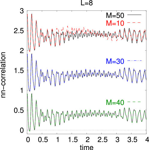
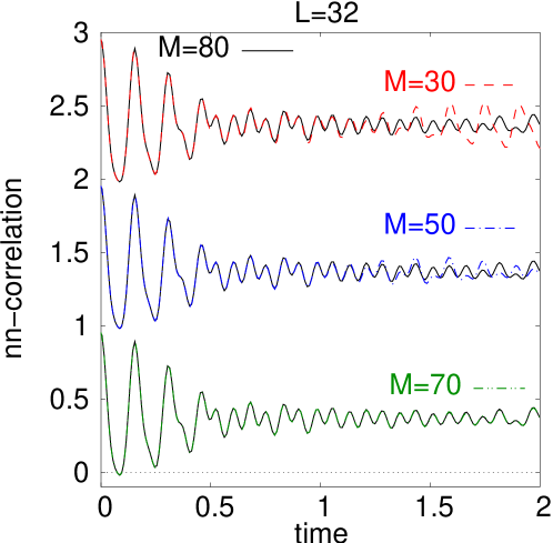
This faster convergence in $M$ enables us to study larger systems than with static time-dependent DMRG (Fig. 9). In the $L=32$ system considered here, we encountered severe convergence problems using static time-dependent DMRG. By contrast, in the new approach convergence sets in for $M$ well below 100, which is easily accessible numerically. Let us remark that the number $M$ of states which have to be kept does certainly vary with the exact parameters chosen, depending if the state can be approximated well by matrix product states of a low dimension. At least in the case studied here, we found that this dependency is quite weak. We expect (also from studying the time evolution of density matrix spectra) that the model dependence of $M$ is roughly similar as in the static case.

Figure 9: Time evolution of the real part of nearest-neighbor correlations in a Bose-Hubard model with instantaneous change of interaction strength using the adaptive time-dependent DMRG but for a larger system $L=32$ with $N=32$ bosons. The different curves for different $M$ are shifted, comparing $M=30,50,70$ to $M=80$ respectively.

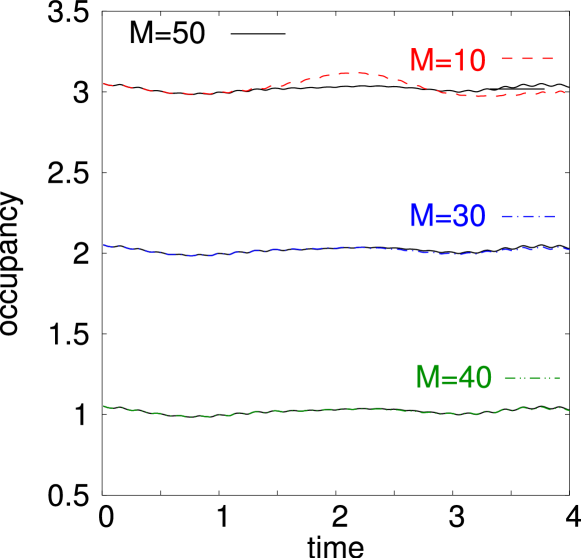
Similar observations are made both for local occupancy (a simpler quantity than nearest-neighbor correlations) and longer-ranged correlations (where we expect less precision). Moving back to the parameter set of section 2, we find as expected that the result for the local occupancy (Fig. 10) is converged for the same $M$ leading to convergence in the nearest-neighbor correlations.

Figure 10: Time evolution of the occupancy of the second site. Parameters as used in section 2 ($L=8$, $N=8$). The different curves for different $M$ are shifted.

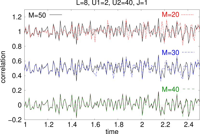
In contrast, if we consider the correlation $\langle b^{\dagger}b\rangle$ between sites further apart from each other the numerical results converge more slowly under an increase of $M$ than the almost local quantities. This can be seen in Fig. 11 where the results for $M=40$ and $M=50$ still differ a bit for times larger than $t\approx 2\hbar/J$.

Figure 11: Time evolution of the real part of the correlation between site 2 and 7. Parameters as used in section 2 with $N=8$ particles. The different curves for different $M$ are shifted. Note that the plot starts at $t=1$ (parameters were changed at $t=0$).

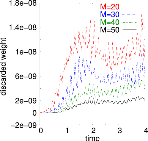
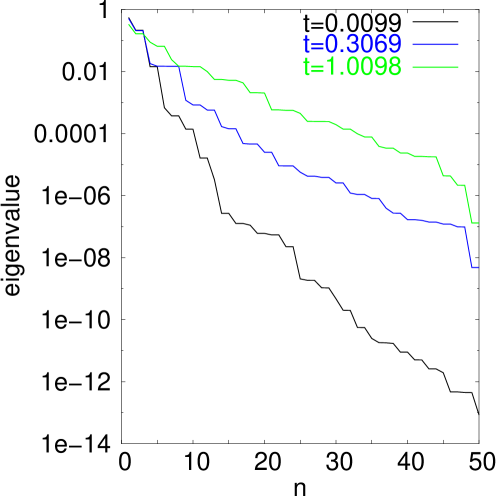
The controlling feature of DMRG is the density matrix formed at each DMRG step – the decay of the density-matrix eigenvalue spectrum and the truncated weight (i.e. the sum of all eigenvalues whose eigenvectors are not retained in the block bases) control its precision. In the discarded weight for the Bose-Hubbard model of section 2 shown in Fig. 12, we can observe that the discarded weight shrinks drastically, going from $M=20$ to $M=50$. This supports the idea that the system shows a fast convergence in $M$. Even more importantly, the discarded weight grows in time, as the state that was originally a ground state at $t<0$ decays into a superposition of many eigenstates of the system at $t>0$. However, in particular for larger $M$, it stays remarkably small throughout the simulation, indicating that adaptive time-dependent DMRG tracks the time-evolving state with high precision. Moving to the detailed spectrum of the density matrix (shown in Fig. 13 for the left density matrix when the chain is symmetrically decomposed into S and E), the corresponding distribution of the eigenvalues can be seen to be approximately exponential. In agreement with the increasing truncation error, one also observes that the decay becomes less steep as time grows. Yet, we still find a comparatively fast decay of the eigenvalue spectrum at all times, necessary to ensure the applicability of TEBD and adaptive time-dependent DMRG respectively.

Figure 12: Discarded weight for different values of $M$. Parameters chosen as in section 2.

Figure 13: Eigenvalue spectrum of the left reduced density matrix at different times for a symmetric S/E decomposition. Parameters chosen as in section 2, $M=50$ states retained.

Note for all results shown that the unusually large number of states per site ($N_{{\rm site}}=14$) which would not occur in Hubbard or Heisenberg models could there be translated directly into longer chains or larger state spaces (larger $M$) for the same computational effort, given that the algorithm is $O(LN_{{\rm site}}^{3}M^{3})$. In that sense, we have been discussing an algorithmically hard case, but in fermionic models DMRG experience tells us that $M$ has to be taken much larger in fermionic systems. For the fermionic Hubbard model, with $N_{{\rm site}}=4$, more than $M=300$ is feasible with the unoptimized code, and much higher $M$ values would be possible if optimizations were carried out. This should be enough to have quantitatively reliable time-evolutions for fermionic chains, while of course not reaching the extreme precision one is used to in DMRG for the static case. As the algorithmic cost is dominated by $(N_{{\rm site}}M)^{3}$, the product $N_{{\rm site}}M$ is an important quantity to look at: while current TEBD implementations range at 100 or less, adaptive time-dependent DMRG using good quantum numbers runs at the order of 1000 (and more).

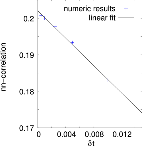
Let us conclude this section by pointing out that at least one improvement can be incorporated almost trivially into this most simple version of adaptive time-dependent DMRG. Since we have used a first-order Trotter decomposition, we expect that for fixed $M$ results of measurements at a fixed time converge linearly with respect to the time step $\delta t$ chosen, as the error per time step scales as $\delta t^{2}$, but the number of time steps needed to reach the fixed time grows as $\delta t^{-1}$. In other words, the Trotter error is inversely proportional to the calculation time spent. This can indeed be observed in results such as presented in Fig. 14.

Figure 14: Convergence in the Trotter time of the real part of the nearest-neighbor correlations between site 2 and 3 in a Bose-Hubbard model with instantaneous change with the parameters chosen as in section 2 at a fixed time.

It is very easily and at hardly any algorithmic cost that a second order Trotter decomposition can be implemented, leading to errors of order $\delta t^{2}$. The second order Trotter decomposition reads[40]

$$e^{-{\rm i}\hat{H}\delta t}=e^{-{\rm i}\hat{H}_{odd}\delta t/2}e^{-{\rm i}\hat{H}_{even}\delta t}e^{-{\rm i}\hat{H}_{odd}\delta t/2},$$ (62)

where we have grouped all local Hamiltonians on odd and even bonds into $\hat{H}_{odd}$ and $\hat{H}_{even}$ respectively. At first sight this seems to indicate that at each Trotter time step three (instead of two) moves (“zips”) through the chain have to be carried out. However, in many applications at the end of most time steps, the Hamiltonian does not change, such that for almost all time steps, we can contract the second $e^{-{\rm i}\hat{H}_{odd}\delta t/2}$ from the previous and the first $e^{-{\rm i}\hat{H}_{odd}\delta t/2}$ from the current time step to a standard $e^{-{\rm i}\hat{H}_{odd}\delta t}$ time step. Hence, we incur almost no algorithmic cost. This is also standard practice in Quantum Monte Carlo [44]; following QMC, second order Trotter evolution is set up as follows:

1. Start with a half-time step $e^{-{\rm i}\hat{H}_{odd}\delta t/2}$.

2. Carry out successive time steps $e^{-{\rm i}\hat{H}_{even}\delta t}$ and $e^{-{\rm i}\hat{H}_{odd}\delta t}$.

3. At measuring times, measure expectation values after a $e^{-{\rm i}\hat{H}_{odd}\delta t}$ time step, and again after a time step $e^{-{\rm i}\hat{H}_{even}\delta t}$, and form the average of the two values as the outcome of the measurement.

4. At times when the Hamiltonian changes, do not contract two half-time steps into one time step.

In this way, additional algorithmic cost is only incurred at the (in many applications rare) times when the Hamiltonian changes while strongly reducing the Trotter decomposition error. Even more precise, but now at an algorithmic cost of factor 5 over the first or second-order decompositions, would be the usage of fourth-order Trotter decompositions (leading to 15 zips through the chain per time step, of which 5, however, can typically be eliminated)[42, 43].

8 Conclusion

The TEBD algorithm for the simulation of slightly entangled quantum systems, such as quantum spin chains and other one-dimensional quantum systems, was originally developed in order to establish a link between the computational potential of quantum systems and their degree of entanglement, and serves therefore as a good example of how concepts and tools from quantum information science can influence other areas of research, in this case quantum many-body physics.

While exporting ideas from one field of knowledge to another may appear as an exciting and often fruitful enterprise, differences in language and background between researchers in so far separated fields can also often become a serious obstacle to the proper propagation and full assimilation of such ideas. In this paper we have translated the TEBD algorithm into the language of matrix product states. This language is a natural choice to express the DMRG algorithm – which, for over a decade, has dominated the simulation of one-dimensional quantum many-body systems. In this way, we have made the TEBD algorithm fully accessible to the DMRG community. On the other hand, this translation has made evident that the TEBD and the DMRG algorithms have a number of common features, a fact that can be exploited.

We have demonstrated that a very straightforward modification of existing finite-system DMRG codes to incorporate the TEBD leads to a new adaptive time-dependent DMRG algorithm. Even without attempting to reach the computationally most efficient incorporation of the TEBD algorithm into DMRG implementations, the resulting code seems to perform systematically better than static time-dependent DMRG codes at very reasonable numerical cost, converging for much smaller state spaces, as they change in time to track the actual state of the system. On the other hand, while it presents no new conceptual idea, the new code is also significantly more efficient than existing embodiments of the TEBD, for instance thanks to the way DMRG handles good quantum numbers. While we have considered bosons as an example, as in standard DMRG fermionic and spin systems present no additional difficulties. Various simple further improvements are feasible, and we think that adaptive time-dependent DMRG can be applied not only to problems with explicitly time-dependent Hamiltonians, but also to problems where the quantum state changes strongly in time, such as in systems where the initial quantum state is far from equilibrium. The method should thus also be of great use in the fields of transport and driven dissipative quantum systems.

Acknowledgments. US and GV would wish to thank the Institute of Theoretical Physics at the University of Innsbruck, where this work was initiated, for its hospitality. CK is supported by the Studienstiftung des Deutschen Volkes and DFG grant DE 730/3-1. The work in Innsbruck is supported by EU networks and the Institute for Quantum Information. GV acknowledges support from the US National Science Foundation under Grant No. EIA-0086038. US acknowledges support by The Young Academy at the Berlin-Brandenburg Academy of Sciences and the Leopoldina Society. We also thank Peter Zoller, Dieter Jaksch, Hans Briegel, Willi Zwerger, Ignacio Cirac, Juanjo Garcia-Ripoll, Miguel Cazalilla, Brad Marston, Jan von Delft and Matthias Troyer for discussions.

Note added in proof. After submission of this work, we became aware of closely related work by White and Feiguin[45].

References

- [1] White S R 1992 Phys. Rev. Lett. 69 2863
- [2] White S R 1993 Phys. Rev. B 48 10345
- [3] Nielsen M A and Chuang I L 2000 Quantum Computation and quantum communication Cambridge University Press
- [4] Osborne T J and Nielsen M A 2002 Quant. Inf. Proc. 1 45 (Osborne T J and Nielsen M A Preprint quant-ph/0109024)
- [5] Dawson C M and Nielsen M A Preprint quant-ph/0401061
- [6] Haselgrowe H L, Nielsen M A and Osborne T J 2003 Preprint quant-ph/0308083
- [7] Vidal G, Latorre J I, Rico E and Kitaev A 2003 Phys. Rev. Lett. 90 227902
- [8] Gaite J 2003 Preprint quant-ph/0301120
- [9] Latorre J I, Rico E and Vidal G 2003 Preprint quant-ph/0304098
- [10] Bennett C H and DiVincenzo D P 2000 Nature 404 247
- [11] Osborne T J and Nielsen M A 2002 Phys. Rev. A 66 032110
- [12] Osterloh A, Amico L, Falci G and Fazio R 2002 Nature 416 608
- [13] Legeza O 2003 Phys. Rev. B 68 195116
- [14] Legeza O 2004 Preprint cond-mat/0401136
- [15] Verstraete F, Popp M, Cirac J I 2004 Phys. Rev. Lett. 92 027901
- [16] Verstraete F, Martin-Delgado M A and Cirac J I 2004 Phys. Rev. Lett. 92 087201
- [17] Vidal G 2003 Preprint quant-ph/0310089
- [18] Peschel I, Wang X, Kaulke M and Hallberg K (eds.) 1999 Density-Matrix Renormalization Springer
- [19] Schollwöck U 2004 Rev. Mod. Phys. submitted
- [20] Cazalilla M A and Marston J B 2002 Phys. Rev. Lett. 88 256403
- [21] Greiner M, Mandel O, Esslinger T, Hänsch T W and Bloch I 2002 Nature 415 39
- [22] Stöferle H et al. 2003 Preprint cond-mat/0312440
- [23] Vidal G 2003 Phys. Rev. Lett. 91 147902
- [24] Jaksch D and Zoller P 2004 in preparation
- [25] Zwolak M and Vidal G 2004 in preparation
- [26] Klümper A, Schadschneider A and Zittartz J 1993 Europhys. Lett. 24 293
- [27] Fannes M, Nachtergaele B and Werner R F 1992 Comm. Math. Phys. 144 3
- [28] White S R 1996 Phys. Rev. Lett. 77 3633
- [29] Press W H et al. 1992 Numerical Recipes in C: The Art of Scientific Computing Cambridge University Press
- [30] Hallberg K 1995 Phys. Rev. B 52 9827
- [31] Kühner T D and White S R 1999 Phys. Rev. B 60 335
- [32] Jeckelmann E 2002 Phys. Rev. B 66 045114
- [33] Luo H G, Xiang T and Wang X Q 2003 Phys. Rev. Lett. 91 049701
- [34] Cazalilla M A and Marston J B 2003 Phys. Rev. Lett. 91 049702
- [35] Östlund S and Rommer S 1995 Phys. Rev. Lett. 75 19
- [36] Dukelsky J, Martín-Delgado M A, Nishino T and Sierra G 1998 Europhys. Lett. 43 457
- [37] Affleck I, Kennedy T, Lieb E H and Tasaki H 1987 Phys. Rev. Lett. 59 799
- [38] Affleck I, Kennedy T, Lieb E H and Tasaki H 1988 Comm. Math. Phys. 115 477
- [39] Fannes M, Nachtergaele B and Werner R F 1989 Europhys. Lett. 10 643
- [40] Suzuki M 1976 Prog. Theor. Phys. 56 1454
- [41] Takasaki H, Hikihara T and Nishino T 1999 J. Phys, Soc. Jpn. 68 1537
- [42] Yoshida H 1990 Phys. Lett. A 150 262
- [43] Krech M, Bunker A and Landau D P 1998 Comp. Phys. Comm. 111 1
- [44] Assaad F F and Würtz D 1991 Phys. Rev. B 44 2681
- [45] White S R 2004 Preprint cond-mat/0403310