Critical Decay at Higher-Order Glass-Transition Singularities

Abstract

Within the mode-coupling theory for the evolution of structural relaxation in glass-forming systems, it is shown that the correlation functions for density fluctuations for states at $A_{3}$- and $A_{4}$-glass-transition singularities can be presented as an asymptotic series in increasing inverse powers of the logarithm of the time $t$: $\phi(t)-f\propto\sum_{i}g_{i}(x)$, where $g_{n}(x)=p_{n}(\ln x)/x^{n}$ with $p_{n}$ denoting some polynomial and $x=\ln(t/t_{0})$. The results are demonstrated for schematic models describing the system by solely one or two correlators and also for a colloid model with a square-well-interaction potential.

1 Introduction

Upon compression or cooling glass-forming liquids, there evolves a peculiar relaxation scenario called glassy dynamics. It is characterized by control-parameter sensitive correlation functions or spectra which are stretched over large intervals of time $t$ or frequency $\omega$, respectively. The so-called mode-coupling theory (MCT) of ideal glass transition has been proposed [1] as a mathematical model for glassy dynamics. The basic version of that theory describes the system by $M$ correlation functions $\phi_{q}(t),\,q=1,\,2,\,\dots,\,M$, which have the meaning of canonically defined auto-correlators of density fluctuations for wave vector moduli $q$ chosen from a grid of $M$ values. The theory deals with a closed set of coupled nonlinear equations of motion for the $\phi_{q}(t)$. The coupling coefficients in these equations are determined by the equilibrium structure factors, which are assumed to be known smooth functions of control parameters like temperature $T$ or density $\rho$. The solution of the MCT equations describe a transition from an ergodic liquid state to a non-ergodic glass state if the control parameters pass critical values $T_{c}$ or $\rho_{c}$, respectively. This transition is accompanied with the appearance of a dynamical scenario, whose qualitative features can be understood by asymptotic solution of the equations for long times and control parameters close to the critical values. The asymptotic formulas establish the universal features of the glassy dynamics described by MCT. On the basis of this understanding, one can construct schematic models. These are based on equations of motion which have the same general form as those derived within the microscopic theory of liquids, but use the number $M$ of correlators and the coupling coefficients as model parameters. Thereby, one gets simplified models whose results can be used for the analysis of data [2].

The ideal liquid-glass transition described by MCT is a fold bifurcation exhibited by the equations of motion. One can show, that all singularities that are generically possible, are of the cuspoid type [3, 4]. Using Arnol’d’s notation [5], an $A_{l}$ is a bifurcation which is equivalent to that for the roots of a real polynomial of degree $l$. Simple schematic models using only a single correlator exhibit besides the fold singularity also the cusp singularity $A_{3}$ and the swallowtail singularity $A_{4}$ [2]. The bifurcation dynamics near a higher-order glass-transition singularity $A_{l},\,l\geqslant 3$, is utterly different from the one near the liquid-glass-transition singularity of type $A_{2}$. A major new feature is the appearance of logarithmic decay yielding to a much stronger stretching than known for the $A_{2}$-scenario [6]. The result for the correlators of $M=1$ models has been worked out in a certain leading-order multiple-scaling-law limit [7]. These formulas have been used to fit dielectric-loss data of glassy polymer melts [8, 9, 10, 11], thereby providing some hint that the MCT for higher-order singularities might be of relevance for understanding glassy dynamics.

Let us consider a system of spherical particles interacting via a steep repulsion potential characterized by a diameter parameter $d$, which is complemented by an attractive potential. The latter shall be characterized by an extension length $\Delta$ and an attraction-potential depth $u_{0}$. Such system is specified conveniently by three control parameters: the packing fraction $\varphi=\rho\pi d^{3}/6$, the dimensionless attraction strength $\Gamma=u_{0}/(k_{\rm B}T)$ or the dimensionless effective temperature $\theta=1/\Gamma$, and the relative attraction width $\delta=\Delta/d$. If $\delta$ is sufficiently large, this potential is a caricature of a van-der-Waals interaction. One gets a decreasing $\Gamma^{c}$-versus-$\varphi^{c}$ line of liquid-glass transitions in the $\Gamma$-$\varphi$ plane of the thermodynamic states similar to what was first calculated within MCT for Lennard-Jones systems [12]. For $\Gamma=0$, the mentioned line terminates at the critical packing fraction $\varphi^{c}_{\rm HSS}$ for the vitrification of the hard-sphere system. The decrease of $\varphi^{c}$ with increasing $\Gamma^{c}$ expresses the intuitive fact that cooling stabilizes the glass state. If $\delta$ is sufficiently small, however, there appear two new phenomena. First, for small $\Gamma$, the $\Gamma^{c}$-versus-$\varphi^{c}$ line increases. Cooling stabilizes the liquid because bond formation creates inhomogeneities which favor fluidity. The new liquid state for $\varphi>\varphi^{c}_{\rm HSS}$ exhibits a reentry phenomenon. Glassification occurs not only by increasing $\Gamma$, i.e. by cooling, but also by decreasing $\Gamma$, i.e. by heating. Second, the $\Gamma^{c}$-versus-$\varphi^{c}$ line can consist of two branches that form a corner. The low-$\Gamma$-branch is terminated by the the high-$\Gamma$-branch. The latter continues into the glass state as glass-glass-transition line, which has an $A_{3}$-singularity as endpoint. These two phenomena have been found by using Baxter’s model for the structure factor as input of the MCT equations [13, 14]. In these calculations, the wave-vector cutoff $q_{\rm max}$ used in the MCT model defines the range parameter $\delta=\pi/(q_{\rm max}d)$. The generic possibility for a transition from small-$\delta$ states with $A_{3}$-singularity to large-$\delta$ states without $A_{3}$-singularity is the appearance of an $A_{4}$-singularity for some critical value $\delta^{*}$. Since the $A_{l}$ bifurcations deal with topological singularities, the indicated scenarios are robust, i.e., they occur for all potentials of the kind specified above. The $A_{4}$-singularity was identified first for the square-well system (SWS), i.e., for a system where a hard-core repulsion is complemented by a shell of constant attraction strength $u_{0}$. Here, $\delta^{*}\approx 0.04$ was calculated [15]. The neighborhood of the $A_{4}$ was analyzed for some other potentials with the conclusion that there are no qualitative differences between results referring to different shapes of the potential or to different approximation schemes for the structure factor [16].

The above described systems with short-ranged attraction can be prepared as colloidal suspensions. The liquid-glass-transition lines can be identified by analyzing the nucleation processes. Light-scattering experiments can provide the density-correlation functions $\phi_{q}(t)$. Such studies have identified the existence of liquid states for $\varphi>\varphi^{c}_{\rm HSS}$ and the reentry phenomenon [17, 18, 19]. Molecular-dynamics simulation studies can determine the mean-squared displacement and the diffusivities with good accuracy. These quantities exhibit drastic precursors of the liquid-glass transition. Several simulation studies [18, 20, 21, 22] have confirmed the predictions on the reentry phenomenon. Near the corner formed by large-$\Gamma$ and the small-$\Gamma$ transition lines, there should occur an almost logarithmic decay of the density correlations $\phi_{q}(t)$, which is followed by a von-Schweidler-law decay as beginning of an $\alpha$-relaxation process [13, 15]. Such scenario was first reported for micellar solutions [23]. This signature of the dynamics for $\varphi>\varphi^{c}_{\rm HSS}$ states was detected also for colloidal suspensions with depletion attraction [19].

In order to identify a higher-order singularity in data from experiment or from molecular-dynamics simulation, one has to identify the features of the correlators $\phi_{q}(t)$ which are characteristic for these singularities. The general theory of the logarithmic decay laws caused by an $A_{l}$ for $l\geqslant 3$, has been developed and the relevant general scenarios have been illustrated for schematic models [24, 25]. The specific implications of the general theory for the SWS, in particular the change of the features with changes of the wave number and the peculiarities expected for the mean-squared displacement, have been worked out as well [26, 27]. Simulation data for the tagged-particle-density correlators as function of the wave vector $q$ [28] provide a first hint that the predicted logarithmic decay processes for $\varphi>\varphi^{c}_{\rm HSS}$ states near an $A_{3}$-singularity are present. Major progress was reported recently for simulation studies for two states of a binary SWS [29]. The logarithmic decay and its expected deformation with wave-number changes has been detected convincingly. The identified amplitudes agree semi-quantitatively with the calculated ones [26]. In addition, the mean-squared displacement exhibits the expected control-parameter dependent power-law behavior. These findings provide very strong arguments for the existence of a higher-order glass-transition singularity. One concludes that the cited MCT results on simple systems with short-ranged attraction reproduce some subtle features of glassy dynamics so that further studies of these systems within that theory seem worthwhile.

If one shifts control parameters towards the ones specifying a higher-order singularity, the time interval for logarithmic decay expands. But, simultaneously, also the beginning of the time interval shifts to larger values. Consequently, there opens a time interval of increasing length between the end of the transient and the beginning of the logarithmic decay. Within this interval, the correlators are close to the critical ones $\phi^{c}_{q}(t)$, i.e., to the correlators calculated for control parameters at the singularity. It should be expected that these critical correlators will be detected in future data from experiments and from simulation studies. It was shown for one-component schematic models that the critical correlators approach their long-time limit proportional to $1/\ln^{m}(t/t_{0})$, where $m=2/(l-2)$ for an $A_{l}$ [7]. In the following, these results shall be extended in two directions. First, the critical correlators shall be expanded in an asymptotic series so that an estimate of the range of validity of various asymptotic formulas is possible. Second, the $\phi_{q}^{c}(t)$ shall be calculated for the general theory so that a discussion of the $q$-dependent corrections of the leading asymptotic formulas is possible for an $A_{3}$- and an $A_{4}$-singularity.

The paper is organized as follows. In Sec. 2, the general starting equations for an asymptotic discussion of critical relaxations are compiled. Then, in Sec. 3 and Sec. 4, the asymptotic expansion is carried out for one-component models for states near an $A_{3}$- and $A_{4}$-singularity, respectively. The results will be demonstrated quantitatively for schematic models. Section 5 shows how the theory for $\phi_{q}^{c}(t)$ for an $A_{3}$ can be reduced to the theory of one-component models, The results are demonstrated for a two-component schematic model and for the SWS. The analogous results for an $A_{4}$-singularity are presented in Sec. 6. A summary is formulated in Sec.7.

2 General equations

2.1 Equations for structural relaxation at glass-transition singularities

Within the basic version of the mode-coupling theory for the evolution of glassy relaxation (MCT), the system’s dynamics is described by $M$ correlators $\phi_{q}(t),\,q=1,\dots,M$. The theory uses the exact Zwanzig-Mori equations of motion. These are specified by $M$ characteristic frequencies $\Omega_{q}>0$ and $M$ fluctuating-force kernels $M_{q}(t)$. The latter are decomposed into regular terms $M^{\rm reg}_{q}(t)$ describing normal-liquid effects and in mode-coupling kernels $m_{q}(t)$. The essential step in the derivation of the theory is the application of Kawasaki’s factorization approximation to express the kernels $m_{q}(t)$ as absolutely monotone functions ${\cal F}_{q}$ of the correlators. These functions depend smoothly on a vector $\mathbf{V}$ of control parameters like density and temperature,

$$m_{q}(t)={\cal F}_{q}[\mathbf{V},\phi_{k}(t)]\,.$$ (1)

Vector $\mathbf{V}$ specifies the equilibrium structure functions of the system. Using Laplace transforms of functions of time, say $F(t)$, to functions defined in the upper plane of complex frequencies $z$, $F(z)=i\int_{0}^{\infty}\,dt\,\exp(izt)\,F(t)$, the equations of motion read $\phi_{q}(z)=-1/\{z-\Omega_{q}^{2}[z+M^{\rm reg}_{q}(z)+\Omega_{q}^{2}m_{q}(z)]\}$ [2]. Glassy dynamics is characterized by long-time decay processes that lead to large small-frequency contributions to $m_{q}(z)$. These small-$z$ contributions to $m_{q}(z)$ dominate over $z+M^{\rm reg}_{q}(z)$. Therefore, glassy dynamics is described by the simplified equation $\phi_{q}(z)=-1/[z-1/m_{q}(z)]$ [30]. Equivalently, there holds $\phi_{q}(z)/[1-z\phi_{q}(z)]=m_{q}(z)$. It will be more convenient to modify the Laplace transform to another invertible mapping ${\cal S}$ from the time domain to the domain of complex frequencies according to

$${\cal S}[F(t)](z)=(-iz)\int_{0}^{\infty}\,dt\,\exp(izt)\,F(t)\,.$$ (2)

Using this notation, the MCT equations for the small-frequency dynamics read

$${\cal S}[\phi_{q}(t)](z)/\{1-{\cal S}[\phi_{q}(t)](z)\}={\cal S}\left[{\cal F}_{q}[\mathbf{V},\phi_{k}(t)]\right](z)\,.$$ (3)

Since ${\cal F}_{q}$ is determined completely by the equilibrium structure functions, the dynamics obtained from Eqs. (1) and (3) is referred to as structural relaxation. These equations are scale invariant: if $\phi_{q}(t)$ is a solution, the same is true for $\phi^{x}_{q}(t)=\phi_{q}(xt)$ for all $x>0$. The scale for the dynamics is determined by the transient motion. The latter is governed by $\Omega_{q}$ and $M^{\rm reg}_{q}(t)$. Since these quantities do not enter Eq. (3), the solutions of Eqs. (1) and (3) are fixed only up to an overall time scale [30]. In the following, this time scale will be denoted by $t_{0}$.

A glass state is characterized by non-vanishing long-time limits of the correlators: $\lim_{t\rightarrow\infty}\phi_{q}(t)=f_{q},\,0<f_{q}<1$. Equivalently, one gets $\lim_{z\rightarrow 0}{\cal S}[\phi_{q}(t)](z)=f_{q}$. Hence, the zero-frequency limit of Eq. (3) yields $f_{q}/(1-f_{q})={\cal F}_{q}[\mathbf{V},f_{k}]$, $q=1,\,2,\,\dots,\,M$. This is a set of $M$ implicit equations to be obeyed by the $M$ numbers $f_{q}$ [1]. If the Jacobian of these equations is invertible, the solutions vary smoothly with changes of $\mathbf{V}$. If the Jacobian is singular for some state $\mathbf{V}^{c}$ with $f_{q}=f_{q}^{c}$, $f_{q}$ exhibits a singularity as function of $\mathbf{V}$ for $\mathbf{V}$ tending towards $\mathbf{V}^{c}$. Therefore, such state $\mathbf{V}^{c}$ is called glass-transition singularity. The solution for the correlators for $\mathbf{V}=\mathbf{V}^{c}$ is referred to as critical correlator $\phi^{c}_{q}(t)$. Let us introduce a functions $\hat{\phi}_{q}(t)$ by

$$\phi^{c}_{q}(t)=f_{q}^{c}+(1-f_{q}^{c})\hat{\phi}_{q}(t)$$ (4)

obeying $\lim_{t\rightarrow\infty}\hat{\phi}_{q}(t)=0$. In the following, $\hat{\phi}_{q}(t)$ and ${\cal S}[\hat{\phi}_{q}(t)](z)$ shall be used as small quantities for an asymptotic expansion of $\phi^{c}_{q}(t)$ for large times and small frequencies. Introducing the coefficients

$$\quad A^{(n)c}_{qk_{1}\dots k_{n}}=\frac{1}{n!}(1-f_{q}^{c})\{\partial^{n}{\cal F}_{q}[\mathbf{V}^{c},f_{k}^{c}]/\partial f_{k_{1}}\cdots\partial f_{k_{n}}\}(1-f_{k_{1}}^{c})\cdots(1-f_{k_{n}}^{c})\,,$$ (5)

Eq. (3) can be rewritten as the set of equations of motion for the $\hat{\phi}_{q}(t)$ [2]:

$$[\delta_{qk}-A^{(1)c}_{qk}]\,{\cal S}[\hat{\phi}_{k}(t)](z)=J_{q}(z)\,.$$ (6)

Here, $J_{q}(z)=\sum_{n\geq 2}J_{q}^{(n)}(z)$ with the $n$th order expansion term given by

$$J_{q}^{(n)}(z)=A^{(n)c}_{qk_{1}\dots k_{n}}{\cal S}[\hat{\phi}_{k_{1}}(t)\cdots\hat{\phi}_{k_{n}}(t)](z)-{\cal S}[\hat{\phi}_{q}(t)]^{n}(z)\,.$$ (7)

In Eq. (6) and  (7) and in all the following equations, summation over pairs of equal labels $k$ is implied. The $M\times M$ matrix $[\delta_{qk}-A^{(1)c}_{qk}]$ is the Jacobian mentioned above. Therefore, a singularity is characterized by matrix $A^{(1)c}_{qk}$ to have an eigenvalue unity. It is a subtle property of the MCT equations that this eigenvalue is non-degenerate and that all other eigenvalues of $A^{(1)c}_{qk}$ have a modulus smaller than unity. The left and right eigenvectors shall be denoted by $a^{*}_{q}$ and $a_{q},\,q=1,\dots,M$, respectively,

$$a^{*}_{k}A^{(1)c}_{kq}=a^{*}_{q}\,,\quad A^{(1)c}_{qk}a_{k}=a_{q}\,.$$ (8)

Generically, one can require $a_{q}\geqslant 0$, $a_{q}^{*}\geqslant 0$ for $q=1,\dots,M$. To fix the eigenvectors uniquely, two normalization conditions can be imposed: $\sum_{q}a^{*}_{q}a_{q}=1,\,\sum_{q}a^{*}_{q}a_{q}a_{q}=1$ [2, 3].

Because of the non-degeneracy mentioned, the singularity is topologically equivalent to that of the zeros of a real polynomial of degree $l,\,l=2,\,3,\dots$. It is a bifurcation of type $A_{l}$ [5]. The singularity can be characterized by a sequence of real coefficients $\mu_{2},\,\mu_{3},\,\dots$. An $A_{l}$ is specified by $\mu_{n}=0$ for $n<l$ and $\mu_{l}\neq 0$. The simplest of these numbers reads

$$\mu_{2}=1-\sum_{q}a^{*}_{q}A^{(2)c}_{qk_{1}k_{2}}a_{k_{1}}a_{k_{2}}\,.$$ (9)

For an $A_{2}$-glass-transition singularity, $\mu_{2}$ determines the so-called critical exponent $a,\,0<a\leq 1/2$. In this case, the critical correlator can be asymptotically expanded as a power series: $\hat{\phi}_{q}(t)=a_{q}(t_{0}/t)^{a}+a^{\prime}_{q}(t_{0}/t)^{2a}+\cdots$ . If the $A_{2}$ singularity approaches a higher-order singularity $A_{l},\,l\geq 3$, the exponent $a$ approaches zero and the cited asymptotic expansion breaks down [2]. It is the goal of this paper to derive a long-time expansion of the critical correlator at $A_{3}$- and $A_{4}$-singularities. Equivalently, it is the aim to solve asymptotically Eqs. (6) and (7) for $\hat{\phi}_{q}(t)$ for states $\mathbf{V}^{c}$ with

$$\mu_{2}=0\,,\quad\mu_{3}\neq 0\,$$ (10a)

for an $$A_{3} \mathbf{V}=\mathbf{V}^{\circ}$$-singularity denoted by and

$$\mu_{2}=\mu_{3}=0\,,\quad\mu_{4}\neq 0\,$$ (10b)

for an $$A_{4} \mathbf{V}=\mathbf{V}^{*}$$-singularity denoted by .

2.2 Expansions of slowly-varying functions

The derivations in this paper shall be based on an extension of the Tauberian theorem for slowly-varying functions, which has been introduced in Ref. [7]. A function $C(t)$ is called of slow variation for long times if $\lim_{T\rightarrow\infty}C(tT)/C(T)=1$ for all $t>0$. This is equivalent to $\gamma(z)={\cal S}[C(t)](z)$ being slowly varying for small frequencies: $\lim_{T\rightarrow\infty}\gamma(z/T)/\gamma(i/T)=1$. In addition, the Tauberian theorem states, that $\gamma(z)$ is asymptotically equal to $G(i/z):\,\lim_{z\rightarrow 0}\gamma(z)/G(i/z)=1$ [31]. Typical examples for functions of slow variation are $p_{m}(\ln(\ln t))/\ln^{m}(t)$, where $m=1,\,2,\,\dots$ and $p_{m}$ denotes some polynomial. The critical correlator $\phi^{c}_{q}(t)$ shall be expressed as sum of such functions. Let us introduce the notations

$$G(t)=g(x)\,,\quad x=\ln(t/t_{0})\,,\quad y=\ln(i/zt_{0})\,,$$ (10ka)

$$g_{m}(x)=p_{m}(x)/x^{m}\,,\quad p_{m}(x)=\sum_{l=0}^{l_{0}}c_{m,l}x^{l}\,.$$ (10kb)

$g_{m+1}(x)$ is asymptotically negligible compared to $g_{m}(x)$: $\lim_{x\rightarrow\infty}g_{m+1}(x)/g_{m}(x)=0$. For later convenience, let us write $f(x)={\cal O}(1/x^{m})$ if $f(x)x^{m}$ is bounded for large $x$ by some polynomial of $\ln x$. Denoting derivatives by $d^{n}g(x)/dx^{n}=g^{(n)}(x),\,n=0,\,1,\,\dots$, one finds

$$g_{m}^{(n)}(x)={\cal O}(1/x^{m+n})\,.$$ (10kl)

Equation (2) can be rewritten as ${\cal S}[G(t)](z)=\int_{0}^{\infty}\,\exp(-u)g(y+\ln u)\,du$. Formal expansion in powers of $\ln u$ leads to

$${\cal S}[G(t)](z)=\sum_{n=0}^{\infty}\frac{1}{n!}\Gamma_{n}g^{(n)}(y)\,.$$ (10km)

Here, $\Gamma_{n}=\Gamma^{(n)}(1)$ denotes the $n$th derivative of the gamma function at unity. One gets $\Gamma_{0}=1,\,-\Gamma_{1}=\gamma$ is Euler’s constant, and $\Gamma_{n}$ for $n\geq 2$ can be expressed in terms of $\gamma$ and Riemann’s zeta-function values $\zeta(K)$ with $K=2,\,\dots,\,n$ [32]. For example, $\Gamma_{2}-\Gamma_{1}^{2}=\zeta(2)$. Using Eq. (10km) with $G(t)=g_{m}(x)$, one gets an asymptotic expansion in terms of increasing order ${\cal O}(1/y^{m+n})$. The leading $n=0$ contribution is $g_{m}(y)$; and this is the result of the Tauberian theorem [31]. The terms for $n\geq 1$ provide systematic improvements for large $y$, i.e. for large times or small frequencies [7].

If one uses Eq. (10km) for $G(t)=G(t)F(t)$, one gets the asymptotic expansion

$${\cal S}[G(t)F(t)](z)-{\cal S}[G(t)](z){\cal S}[F(t)](z)=\sum_{n=2}^{\infty}\sum_{m=1}^{n-1}\frac{[\Gamma_{n}-\Gamma_{n-m}\Gamma_{n}]}{(n-m)!m!}g^{(n-m)}(y)f^{(m)}(y).$$ (10kn)

Let us use $G(t)=g_{m_{1}}(x)$ and $F(t)=g_{m_{2}}(x)$. The Tauberian theorem implies that the leading contribution to ${\cal S}[G_{m_{1}}(t)G_{m_{2}}(t)](z)$ cancels against the leading contribution to ${\cal S}[G_{m_{1}}(t)](z){\cal S}[G_{m_{2}}(t)](z)$. The tricks underlying the asymptotic solution of the MCT equations at a higher-order singularity are based on the observation that also the leading corrections to the Tauberian theorem cancel [7]:

$$\qquad{\cal S}[g_{m_{1}}(t)g_{m_{2}}(t)](z)-{\cal S}[g_{m_{1}}(t)](z){\cal S}[g_{m_{2}}(t)](z)={\cal O}(1/y^{m_{1}+m_{2}+2})\,.$$ (10ko)

The difference between the two terms on the left-hand side is two orders smaller for vanishing frequencies than each of the terms separately.

3 Critical correlators for one-component models at an $A_{3}$-singularity

3.1 The leading contribution

It will be shown in Sec. 5 how one can reduce the problem of solving Eqs. (6) and (7) for a general number $M$ of the correlators to the special problem of solving for $M=1$ models. Therefore, the problem shall be discussed first for one-component models. For this case, one can drop the indices in all formulas of Sec. 2.1. There is only one correlator $\phi^{c}(t)$, one long-time limit $f^{c}$ for the critical point $\mathbf{V}^{c}$, and one function $\hat{\phi}(t)$ determining the critical correlator as $\phi^{c}(t)=f^{c}+(1-f^{c})\hat{\phi}(t)$. The Jacobian matrix agrees with its eigenvalue, and this is zero. Hence, Eqs. (6) and (7) can be noted as

$$K(z)=0\,,$$ (10kpa)

$$K(z)=\sum_{n=2}^{\infty}K_{n}(z)\,.$$ (10kpb)

Here, $K_{n}(z)$ is the expansion term of order $\hat{\phi}^{n}$. Let us introduce the abbreviation

$$\psi_{n}(z)={\cal S}[\hat{\phi}^{n}(t)](z)-{\cal S}[\hat{\phi}(t)]^{n}(z)\,,$$ (10kpq)

and denote its inverse transform by $\psi_{n}(t)$, i.e., ${\cal S}[\psi_{n}(t)](z)=\psi_{n}(z)$. Remembering that for $M=1$ models there holds $\mu_{n}=1-A^{(n)c}$, one gets $K_{n}(z)=\psi_{n}(z)-\mu_{n}{\cal S}[\hat{\phi}^{n}(t)](z)$ [24]. Specializing to the $A_{3}$-singularity as noted in Eq. (10a), the equation of motion (10kpa) is defined by

$$\begin{array}[]{ll}K(z)=&\psi_{2}(z)-\mu_{3}{\cal S}[\hat{\phi}^{3}(t)](z)\\ &+\kappa\psi_{3}(z)-\mu_{4}{\cal S}[\hat{\phi}^{4}(t)](z)\\ &+K^{\prime}(z)\,.\end{array}$$ (10kpr)

Here, $K^{\prime}(z)=\kappa^{\prime}\psi_{4}(z)-\mu_{5}{\cal S}[\hat{\phi}^{5}(t)](z)+\dots$. The numbers $\kappa$ and $\kappa^{\prime}$ have been introduced for later convenience. For the $M=1$ models under consideration, one has to substitute $\kappa=\kappa^{\prime}=1$.

Let us examine whether one can solve the equations with the Ansatz $\hat{\phi}(t)=g_{m}(x)=c_{m}/x^{m}$. From Eq. (10km) one gets ${\cal S}[\hat{\phi}^{3}(t)](z)=(c_{m}/y^{m})^{3}+{\cal O}(1/y^{3m+1})$. Using Eq. (10kn) with $G(t)=F(t)=g_{m}(x)$, one obtains $\psi_{2}(z)=\zeta(2)(mc_{m}/y^{m+1})^{2}+{\cal O}(1/y^{2m+3})$. Choosing $m=2$, both terms in the first line of Eq. (10kpr) are of the same order $1/y^{6}$. They cancel in this leading order if $\mu_{3}c_{2}^{3}=4\zeta(2)c_{2}^{2}$. From Eqs. (10km) and (10ko) one infers that the terms in the second line of Eq. (10kpr) are of order $1/y^{8}$ and $K^{\prime}={\cal O}(1/y^{10})$. One concludes that the leading asymptotic behavior of the critical correlator for large times is described by $\hat{\phi}(t)=g_{2}(x)$, where

$$g_{2}(x)=c_{2}/x^{2}\,,\quad c_{2}=4\zeta(2)/\mu_{3}\,.$$ (10kps)

3.2 The leading correction

Let us split the function $\hat{\phi}(t)$ into its leading term and a correction $\tilde{g}(x)$:

$$\hat{\phi}(t)=g_{2}(x)+\tilde{g}(x)\,.$$ (10kpt)

Substitution of this formula into the first line of Eq. (10kpr), one gets expressions up to third order in $\tilde{g}$. The term independent of $\tilde{g}$ is ${\cal S}[g_{2}^{2}(x)](z)-{\cal S}[g_{2}(x)]^{2}(z)-\mu_{3}{\cal S}[g_{2}^{3}(x)](z)$, and it shall be denoted by $[(4\zeta(2))^{2}/\mu_{3}]F(y)$. Equations (10km) and (10kn) are used to derive the asymptotic series

$$\qquad F(y)=\sum_{n=3}^{\infty}\frac{(-1)^{n+1}}{\mu_{3}y^{4+n}}\left\{\frac{1}{30}\zeta(2)\frac{(n+3)!}{(n-2)!}\Gamma_{n-2}\right.$$

$$-\left.\sum_{m=1}^{n-2}(n-m+1)(m+1)(\Gamma_{n}-\Gamma_{n-m}\Gamma_{m})\right\}.$$ (10kpua)

The term linear in $$\tilde{g} 2\{{\cal S}[g_{2}(x)\tilde{g}(x)](z)-{\cal S}[g_{2}(x)](z){\cal S}[\tilde{g}(x)](z)\}-3\mu_{3}{\cal S}[g_{2}^{2}(x)\tilde{g}(x)](z) [(4\zeta(2))^{2}/\mu_{3}][{\cal D}\tilde{g}(y)+{\cal D}^{\prime}\tilde{g}(y)] {\cal D}$$ is . It shall be denoted by . Here, the differential operator yields the leading contribution

$${\cal D}\tilde{g}(y)=[y\cdot d\tilde{g}(y)/dy+3\tilde{g}(y)]/y^{4}\,.$$ (10kpub)

The correction $${\cal D}^{\prime}$$ is expanded with the aid of Eqs. (10km) and (10kn):

$$\quad{\cal D}^{\prime}\tilde{g}(y)=[1/2\zeta(2)]\sum_{n=3}^{\infty}\sum_{m=1}^{n-1}(-1)^{n-m}\left\{[\tilde{g}^{(m)}(y)/y^{n+2-m}m!](\Gamma_{n}-\Gamma_{n-m}\Gamma_{m})\right.$$

$$\qquad\left.+\zeta(2)\Gamma_{n-2}[\tilde{g}^{(m-1)}(y)/y^{n+3-m}(m-1)!](n-m+1)(n-m)(n-m+1)\right\}\,.$$ (10kpuc)

With these notations, the equation of motion for $\tilde{g}(y)$ is reformulated as a linear differential equation with some inhomogeneity $I(y)$:

$${\cal D}\tilde{g}(y)=I(y)\,,$$ (10kpuva)

$$I(y)= F(y)+{\cal D}^{\prime}\tilde{g}(y)$$ (10kpuvb)

$$+{\cal S}[\tilde{g}^{2}(x)](z)-{\cal S}[\tilde{g}(x)]^{2}(z)-3\mu_{3}{\cal S}[g_{2}(x)\tilde{g}^{2}(x)](z)$$

$$-\mu_{3}{\cal S}[\tilde{g}^{3}(x)](z)+\kappa\psi_{3}(z)-\mu_{4}{\cal S}[\hat{\phi}^{4}(t)](z)+K^{\prime}(z)\,.$$

It might be adequate to emphasize, that Eqs. (10kps)–(10kpuvb) formulate an exact rewriting of Eq. (3) for $M=1$ models.

The iterative solution of Eq. (10kpuva ) for $\tilde{g}(x)$ is based on the observation, that one gets for functions $g_{m}(y)$ from Eq. (10kb):

$${\cal D}g_{m}(y)=[p_{m}^{\prime}(y)+(3-m)p_{m}]/y^{m+4}\,.$$ (10kpuvw)

If one tries with $\tilde{g}(x)=g_{3}(x)$, one finds on the one hand ${\cal D}g_{m}(y)=p_{3}^{\prime}(y)/y^{7}$. On the other hand, one verifies, that all terms on the right hand side of Eq. (10kpuvb) are ${\cal O}(1/y^{8})$ except for the $n=4$ contribution to $F(y)$. One checks that $F(y)=24\zeta(3)/(\mu_{3}y^{7})+{\cal O}(1/y^{8})$. Hence, the leading order solution for $\tilde{g}$ reads

$$g_{3}(x)=c_{3}\ln(x)/x^{3}\,,\quad c_{3}=24\zeta(3)/\mu_{3}\,.$$ (10kpuvx)

Combining this finding with Eqs. (10kps) and (10kpt) and eliminating all the abbreviations, one reproduces a result of Ref. [7]:

$$\qquad\phi^{\circ}(t)=f^{\circ}+(1-f^{\circ})[c_{2}/\ln^{2}(t/t_{0})]\left\{1+[6\zeta(3)/\zeta(2)]\ln\ln(t/t_{0})/\ln(t/t_{0})\right\}\,.$$ (10kpuvy)

This formula describes the critical correlator up to errors of the order $1/\ln^{4}(t/t_{0})$.

3.3 Higher-order contributions

The equation for $\tilde{g}(y)$ allows for an iterative solution so that the iteration step with number $m$ reads $\tilde{g}=g_{3}+g_{4}+\cdots+g_{m}$. Here the numerator polynomial in Eq. (10kb) is of degree not larger than $(m-2)$, i.e.,

$$g_{m}(x)=\sum_{l=0}^{m-2}c_{m,l}\ln^{l}(x)/x^{m}\,.$$ (10kpuvz)

Suppose, the procedure had been carried out up to step $m-1,\,m=4,\,5,\dots$. Then ${\cal D}\tilde{g}(y)={\cal D}g_{m}(y)+{\cal O}(1/y^{m+3})$. By construction, all terms up to order $(m+3)$ cancel against the one appearing in $I(y)$. One checks, that the leading contribution to $I(y)$ reads $p(\ln y)/y^{m+4}$, where the degree of the polynomial $p$ does not exceed $m-3$. Hence, Eq. (10kpuva) is equivalent to the linear differential equation $p_{m}^{\prime}+(3-m)p_{m}=p$. It is readily solved by Eq. (10kpuvz), provided the coefficients $c_{m,l}$ are chosen properly.

In order to determine $g_{4}$ and $g_{5}$, one can drop $K^{\prime}(z)$ in Eq. (10kpuvb). The coefficients $c_{m,l}$ are given by $\mu_{3}$, $\kappa$, and $\mu_{4}$ as follows

$$\qquad c_{4,0} = 792\zeta(3)^{2}/(\pi^{2}\mu_{3})+[4\mu_{4}/(9\mu_{3}^{2})-4\kappa/(3\mu_{3})-7/6]\,\pi^{4}/\mu_{3}\,,$$ (10kpuvaaa)

$$\qquad c_{4,1} = -432\zeta(3)^{2}/(\pi^{2}\mu_{3})\,,$$ (10kpuvaab)

$$\qquad c_{4,2} = 648\zeta(3)^{2}/(\pi^{2}\mu_{3})\,,$$ (10kpuvaac)

$$\qquad c_{5,0} = \zeta(3)\pi^{2}[400\kappa\mu_{3}+1551\mu_{3}^{2}-160\mu_{4}]/(15\mu_{3}^{3})$$

$$-[39744\,\zeta(3)^{3}/\pi^{4}+528\zeta(5)]/\mu_{3}\,,$$ (10kpuvaaaba)

$$\qquad c_{5,1} = 64800\,\zeta(3)^{3}/(\pi^{4}\mu_{3})-4\zeta(3)\pi^{2}(21\mu_{3}^{2}-24\kappa\mu_{3}+8\mu_{4})/\mu_{3}^{3}\,,$$ (10kpuvaaabb)

$$\qquad c_{5,2} = -27216\,\zeta(3)^{3}/(\pi^{4}\mu_{3})\,,$$ (10kpuvaaabc)

$$\qquad c_{5,3} = 15552\,\zeta(3)^{3}/(\pi^{4}\mu_{3})\,,$$ (10kpuvaaabd)

The coefficients for $g_{6}$ and $g_{7}$ have also been determined . The only new model parameters entering the coefficients are $\mu_{5}$ and $\kappa^{\prime}$ [33].

3.4 Discussion

The preceding results shall be demonstrated quantitatively for the simplest model exhibiting a generic $A_{3}$-glass-transition singularity. This model was derived for a spin-glass system and it is defined by the mode-coupling function [34]

$$m(t)=v_{1}\phi(t)+v_{3}\phi^{3}(t)\,.$$ (10kpuvaaabac)

Here and in the following models, we use a Brownian short-time dynamics as specified by the equation of motion

$$\tau\partial_{t}\phi(t)+\phi(t)+\int_{0}^{t}\,dt^{\prime}m(t-t^{\prime})\partial^{\prime}_{t}\phi(t^{\prime})=0\,,$$ (10kpuvaaabad)

to be solved with the initial condition $\phi(t\rightarrow 0)=1$. The short-time asymptote is $\phi(t)-1=-(t/\tau)+{\cal O}((t/\tau)^{2})$. The singularity is obtained for the coupling constants $v_{1}^{\circ}=9/8$ and $v_{3}^{\circ}=27/8$. The critical long-time limit of the correlator is $f^{\circ}=1/3$ [24, 6]. The other parameters entering the coefficients via Eqs. (10kpuvaa) and (10kpuvaaab) are $\mu_{3}=1/3$ and $\mu_{4}=\mu_{5}=\kappa=\kappa^{\prime}=1$. Thus, all expansion formulas are specified, except for the time scale $t_{0}$. To ease reference to various degrees of asymptotic expansions, let us introduce the abbreviation for the $n$th order approximation

$$\phi^{\circ}(t)_{n}=f^{\circ}+(1-f^{\circ})\,G_{n}(t)\,,\quad G_{n}(t)=\sum_{m=2}^{n}g_{m}(\ln(t/t_{0}))\,.$$ (10kpuvaaabae)

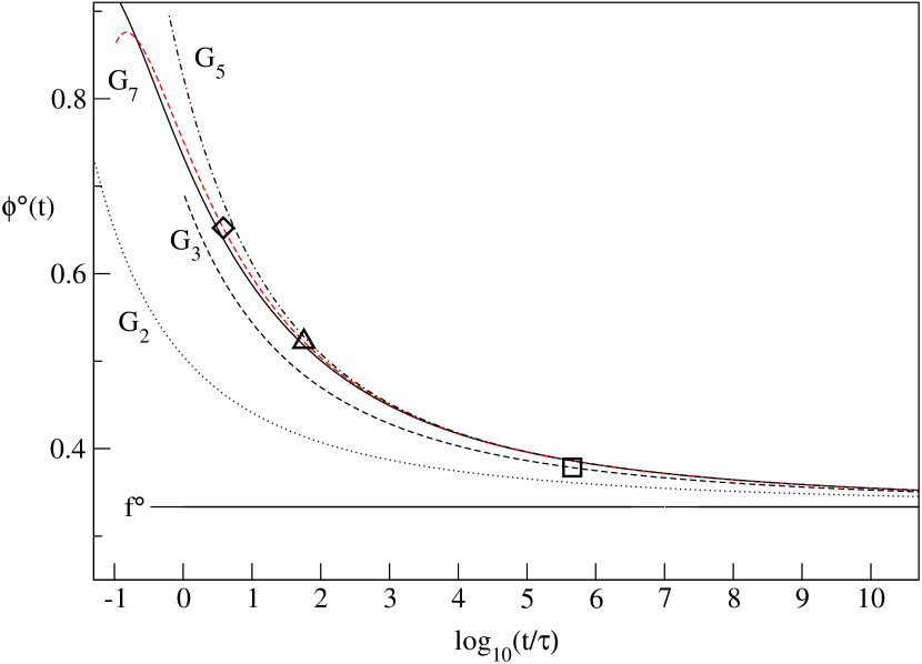
Figure 1: Critical decay at the $A_{3}$-singularity of the model defined by Eqs. (10kpuvaaabac) and (10kpuvaaabad). The full line shows the solution for $\phi^{\circ}(t)$. The lines labeled $G_{n}$, for $n=2,\,3,\,5,\,7$, show the approximations from Eq. (10kpuvaaabae) with the time scale $t_{0}/\tau=1.6\cdot 10^{-4}$. The time where $G_{3}$, $G_{5}$, and $G_{7}$ deviate by $2\%$ from $\phi^{\circ}(t)$ is marked by a square ($\square$), a triangle ($\triangle$), and a diamond ($\diamond$), respectively.

Figure 1 exhibits $\phi^{\circ}(t)$ as obtained from Eqs. (10kpuvaaabac) and (10kpuvaaabad) for the state $\mathbf{V}=\mathbf{V}^{\circ}$. The approach to the critical plateau $f^{\circ}$ is significantly slower than the one for a typical $A_{2}$-singularity. In the latter case, the decay comes close to the plateau within a few decades of increase of the time when a deviation of $5\%$ is used as a measure. Such a criterion is not met by the decay in Fig. 1 for the entire window in time shown. For $t=10^{11}$, the critical correlator $\phi^{\circ}(t)$ is still $5.5\%$ above $f^{\circ}$. To apply the asymptotic approximation, one has to match the time scale $t_{0}$ at large times. A reliable determination of $t_{0}$ is not possible when using only $G_{2}(x)$ or $G_{3}(x)$. Using $G_{7}(x)$ and extending the numerical solution to $t/\tau=10^{38}$, it is possible to fix $t_{0}/\tau=1.6\cdot 10^{-4}$. Notice, that $t_{0}$ is several orders of magnitude smaller than the time scale $\tau$ for the transient dynamics. With this value for $t_{0}$, the successive asymptotic approximations are shown in Fig. 1. The leading approximation from Eq. (10kpuvaaabae), labeled $G_{2}$, deviates from the critical correlator strongly. Including the next-to-leading term $g_{3}(x)$ yields the approximation labeled $G_{3}$, i.e. Eq. (10kpuvy). A square indicates that $G_{3}$ deviates from the critical correlator by less than $2\%$ for $t/\tau\gtrsim 5\cdot 10^{5}$. If that criterion is relaxed to $5\%$, $G_{3}$ obeys it for $t\gtrsim 10^{3}\tau$. The approximation by $G_{3}$ provides a first reasonable approximation to $\phi^{\circ}(t)$. Including further terms of the expansion improves the approximation as is shown for $G_{5}$ and $G_{7}$. One recognizes that proceeding from $G_{5}$ to $G_{7}$ still improves the range of applicability by one order of magnitude in time. We conclude that the asymptotic expansion explains quantitatively the critical decay at the $A_{3}$-singularity for all times outside the transient regime.

Figure 2: Time scale $t_{0}$ in units of $\tau$ for the approximation of the critical decay at the $A_{3}$-singularity of the model studied in Fig. 1 by including $n$ orders of the asymptotic expansion, Eq. (10kpuvaaabae). Time scales obtained by matching $G_{7}(t)$ at large time, $35\lesssim\log_{10}t\lesssim 38$ are shown by crosses ($\times$). The time $t^{\prime}_{0}$ resulting from matching the solutions at $t=10^{6}$ is shown by filled circles ($\bullet$). The diamonds ($\diamond$) show the time scale $t_{0}^{\prime\prime}$ resulting from matching where $\phi(t)=2/3$. The inset shows $t_{0}$ on logarithmic scale. The lines are guide to the eye.

Matching a time scale $t_{0}$ at $t/\tau=10^{40}$ and using six terms of the expansion in Eq. (10kpuvaaabae) is not a promising perspective for fitting data. However, the expansion leads to a reasonable approximation also for short times. Therefore, we may depart from the procedure to match $t_{0}$ at large times and try to fit $t_{0}$ for shorter times. Figure 2 shows as crosses the values obtained for $t_{0}$ when matching the approximations at the large times mentioned above. We will consider two procedures for fitting. The first shall define a scale $t_{0}^{\prime}$ by matching the critical correlator by the approximation at $t=10^{6}$. The second time scale $t_{0}^{\prime\prime}$ is obtained from matching at $50\%$ of the decay, i.e. for the time $t^{*}$ where $\phi^{\circ}(t^{*})=2/3$. We infer from the inset of Fig. 2 that all methods to fix $t_{0}$ based on the term $G_{2}(x)$ alone are off by orders of magnitude. The approximation $G_{3}(x)$ yields the correct order of magnitude for $t_{0}$ in all three approaches. Starting with $n=5$, the scales $t_{0}$ and $t^{\prime}_{0}$ can no longer be distinguished. Therefore, matching the approximation at $10^{6}$ is comparable to matching a true asymptotic limit. The value $t_{0}^{\prime}$ is a better approximation for $t_{0}$ than $t_{0}^{\prime\prime}$.

4 Critical correlators for one-component models at an $A_{4}$-singularity

Within the theory of the logarithmic decay as presented in Ref. [24], it is possible to specialize to the $A_{4}$-singularity by simply setting $\mu_{3}=0$ in the final formulas. Different from that, the critical decay for the $A_{4}$-singularity does not follow from the solution for the $A_{3}$-singularity but requires a different asymptotic expansion. This can be inferred from the fact that all the coefficients $c_{m,l}$ in Eq. (10kpuvz) contain $\mu_{3}$ in the denominator. However, the tricks used for finding a solution in terms of slowly varying functions are the same for the $A_{4}$ as explained above for the $A_{3}$.

4.1 The leading contribution

Using Eq. (10b) for an $A_{4}$-singularity, Eqs. (10kpa) and (10kpr) can be regrouped as

$$\begin{array}[]{cccc}0=&\psi_{2}(z)&-&\mu_{4}\,{\cal S}[\hat{\phi}^{4}(t)](z)\\ \quad+&\kappa\psi_{3}(z)&-&\mu_{5}\,{\cal S}[\hat{\phi}^{5}(t)](z)\\ \quad+&\kappa^{\prime}\psi_{4}(z)&-&\mu_{6}\,{\cal S}[\hat{\phi}^{6}(t)](z)\\ &&&+\qquad\dots\,\,.\end{array}$$ (10kpuvaaabaf)

With the Ansatz $\hat{\phi}(t)=g_{m}(x)=c_{m}/x^{m}$, one arrives for the terms of the first line at $\psi_{2}(z)=\zeta(2)(mc_{m}/y^{m+1})^{2}+{\cal O}(1/y^{2m+3})$ and ${\cal S}[\hat{\phi}^{4}(t)](z)=(c_{m}/y^{m})^{4}+{\cal O}(1/y^{4m+1})$. For $m=1$, the first line in Eq. (10kpuvaaabaf) is of leading order ${\cal O}(1/y^{4})$ with the equation for the coefficient $\zeta(2)c_{1}^{2}=\mu_{4}c_{1}^{4}$. This results in the leading-order solution [7],

$$g_{1}(x)=c_{1}/x\,,\quad c_{1}=\sqrt{\zeta(2)/\mu_{4}}\,.$$ (10kpuvaaabag)

4.2 The leading correction

The corrections may be rephrased in terms of a differential operator and the solution is straight forward as before. Since later on, only the first correction will be needed explicitly, it will be calculated here by the linear differential equation for the Ansatz $\hat{\phi}(t)=\left[\phi^{*}(t)-f^{*}\right]/(1-f^{*})=g_{1}(x)+\tilde{g}(x)$,

$$\qquad 2y^{3}\tilde{g}^{\prime}(y)+4y^{2}\tilde{g}=4\sqrt{\zeta(2)/\mu_{4}}\,\zeta(3)/\zeta(2)+3\zeta(2)\kappa/\mu_{4}-\mu_{5}\zeta(2)/\mu_{4}^{2}\,.$$ (10kpuvaaabah)

This is solved in leading order by $g_{2}(x)$:

$$g_{2}(x)=c_{2}\ln(x)/x^{2}\,,\quad c_{2}=2\sqrt{\zeta(2)/\mu_{4}}\,\zeta(3)/\zeta(2)+3\zeta(2)\kappa/(2\mu_{4})-\mu_{5}\zeta(2)/(2\mu_{4}^{2})\,.$$ (10kpuvaaabai)

Higher-order contributions for $m\geqslant 3$ can be written in the form

$$g_{m}(x)=\sum_{l=0}^{m-1}c_{m,l}\ln^{l}(x)/x^{m}$$ (10kpuvaaabaj)

with the appropriate choice of the parameters $c_{m,l}$. Hence, the general solution for the critical decay at an $A_{4}$-singularity in the one-component case is represented up to errors of order ${\cal O}(\ln^{-(n+1)}(t)$ as

$$\phi(t)^{*}=f^{*}+(1-f^{*})\,G_{n}(t)\,,\quad G_{n}(t)=\sum_{m=1}^{n}g_{m}(\ln(t/t_{0}))\,.$$ (10kpuvaaabak)

Because the leading order result $g_{1}(x)$ is of order ${\cal O}(1/\ln t)$ each higher order solution requires the inclusion of an additional line in Eq. (10kpuvaaabaf). This adds new parameters like $\mu_{6}$ and $\kappa^{\prime}$ in each step, whereas for the $A_{3}$-singularity, Eq. (10kpuvz), additional parameters occur only in every second step of the expansion.

4.3 Discussion

The results for the $A_{4}$-singularity shall be demonstrated for the kernel [6],

$$m(t)=v_{1}\phi(t)+v_{2}\phi^{2}(t)+v_{3}\phi^{3}(t)\,,$$ (10kpuvaaabal)

substituted into the equation of motion (10kpuvaaabad) used with $\tau=1$. The model has an $A_{4}$-singularity at $\mathbf{V}^{*}=(1,1,1)$ with $f^{*}=0$ and coefficients $\mu_{l},\,l\geqslant 4$ and $\kappa$ being unity.

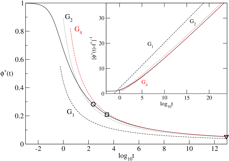
Figure 3: Critical decay $\phi^{*}(t)$ at the $A_{4}$-singularity of the model defined by Eqs. (10kpuvaaabad) and (10kpuvaaabal), and the unit of time chosen such that $\tau=1$. The approximations by Eq. (10kpuvaaabak) with $t_{0}=0.055$ matched for $G_{4}$ are labeled accordingly. The square and the circle mark the time where the approximation by $G_{4}$ deviates from the solution by $5\%$ and $10\%$, respectively. The triangle refers to a $5\%$ deviation of $G_{2}$ from the solution. The inset displays the inverse of $[\phi^{*}(t)-f^{*}]$ and its respective approximations.

Using up to four terms in the expansion (10kpuvaaabak), the time scale is fixed at $t_{0}=0.055$. Successive approximations to the numerical solution are shown in Fig. 3. Again, the leading approximation $G_{1}$ does not describe the solution. The inset shows $[\phi^{*}(t)-f^{*}]^{-1}$, where a decay proportional to $1/\ln t$ would be seen as a straight line. $G_{1}$ yields such a straight line by definition; but it has the wrong slope compared to the solution. The latter exhibits a straight line for $t\gtrsim 10^{7}$. Including the leading correction in $G_{2}$ can account for the slope of the long-time solution. Further terms in the asymptotic expansion enhance the accuracy of the approximation. $G_{4}$ fulfills the $5\%$ criterion at $t=3\,10^{3}$, and is in accord with the solution on the $10\%$ level for $t>230$. $G_{2}$ intersects $\phi^{*}(t)$ for shorter times but deviates first from the solution by $5\%$ at $t=9\cdot 10^{12}$.

5 Asymptotic expansion of the critical correlators at an $A_{3}$-singularity

For the study of the general models, we go back to Eqs. (4–7). The solvability condition for Eq. (6) reads

$$\sum_{q}a^{*}_{q}J_{q}(z)=0\,\,,$$ (10kpuvaaabama)

and the general solution can be written as

$$\hat{\phi}_{q}(t)=a_{q}\hat{\phi}(t)+\tilde{\phi}_{q}(t)\,\,.$$ (10kpuvaaabamb)

The splitting of $$\hat{\phi}_{q}(t) \sum_{q}a^{*}_{q}\,\hat{\phi}_{q}(t)=\hat{\phi}(t) \tilde{\phi}_{q}(t) R_{qk} A_{qk}^{(1)c}$$ in two terms is unique if one imposes the convention . Then, the part can be expressed by means of the reduced resolvent of :

$${\cal S}[\tilde{\phi}_{q}(t)](z)=R_{qk}J_{k}(z)\,\,.$$ (10kpuvaaabamc)

The matrix $R_{qk}$ can be evaluated from matrix $A_{qk}^{(1)c}$ and the vectors $a^{*}_{k},\,a_{k}$ [35]. Let us emphasize that Eqs. (10kpuvaaabama–c) together with the definitions in Eqs. (4) and (7) are an exact reformulation of the equation of motion (3) for states at glass-transition singularities. It is the aim of following calculations to express $\tilde{\phi}_{q}(t)$ recursively in terms of $\hat{\phi}(t)$ and to show that $\hat{\phi}(t)$ has the asymptotic expansion discussed in Sec. 3 for the one-component models. The starting point is the observation that $\tilde{\phi}_{q}(t)$ is small of higher order than $\hat{\phi}(t)$. This is obvious, since Eqs.(7) and (10kpuvaaabamc) imply $\tilde{\phi}_{q}(z)={\cal O}(\hat{\phi}^{2})+{\cal O}(\hat{\phi}\tilde{\phi}_{q})+{\cal O}(\tilde{\phi}_{q}^{2})$. Therefore, one gets

$$J_{q}(z)={\cal O}(\hat{\phi}^{2})\,,$$ (10kpuvaaabamana)

$$\tilde{\phi}_{q}(t)={\cal O}(\hat{\phi}^{2})\,.$$ (10kpuvaaabamanb)

We assume that $\hat{\phi}$ can be expanded in terms of functions $g_{m}(x)$ as defined in Eqs. (10ka,b), and show the legitimacy of this Ansatz by the success of the following constructions.

5.1 Expansion up to next-to-leading order

Substituting the splitting (10kpuvaaabamb) into the inhomogeneity $J^{(2)}_{q}(z)$ from Eq. (7) yields

$$J_{q}(z)=A^{(2)c}_{qk_{1}k_{2}}a_{k_{1}}a_{k_{2}}{\cal S}[\hat{\phi}(t)^{2}](z)-a_{q}^{2}{\cal S}[\hat{\phi}(t)]^{2}(z)+{\cal O}(\hat{\phi}^{3})\,.$$ (10kpuvaaabamanao)

The function $\psi_{2}(z)$ in Eq. (10kpq) is of order ${\cal O}(\hat{\phi}^{3})$ because of Eq. (10ko). Therefore,

$$J_{q}(z)=(A^{(2)c}_{qk_{1}k_{2}}a_{k_{1}}a_{k_{2}}-a_{q}^{2})\,{\cal S}[\hat{\phi}(t)^{2}](z)+{\cal O}(\hat{\phi}^{3})\,.$$ (10kpuvaaabamanap)

Remembering Eq. (9) and the condition $\mu_{2}=0$, one notices that the solvability condition (10kpuvaaabama) is fulfilled to order ${\cal O}(\hat{\phi}^{2})$. Hence, Eq. (10kpuvaaabamc) yields

$$\tilde{\phi}_{q}(t)=X_{q}\hat{\phi}^{2}(t)+{\cal O}(\hat{\phi}^{3})$$ (10kpuvaaabamanaq)

with the abbreviation [24]

$$X_{q}=R_{qk}\left[A_{kk_{1}k_{2}}^{(2)c}a_{k_{1}}a_{k_{2}}-a_{k}^{2}\right]\,\,.$$ (10kpuvaaabamanar)

The first step in the derivation of $q$-dependent corrections results in the extension of Eq. (10kpuvaaabamb):

$$\hat{\phi}_{q}(t)=a_{q}\hat{\phi}(t)+X_{q}\hat{\phi}^{2}(t)+\tilde{\phi}^{\prime}_{q}(t)\,,$$ (10kpuvaaabamanasa)

where

$$\tilde{\phi}^{\prime}_{q}(t)={\cal O}(\hat{\phi}^{3})\,.$$ (10kpuvaaabamanasb)

The next step is started by substituting the result (10kpuvaaabamanasa) into Eq. (7) for $J_{q}(z)$. Terms of order ${\cal O}(\hat{\phi}^{2})$ vanish altogether as demonstrated above and only $a_{q}^{2}\psi_{2}(z)$ and additional terms of order ${\cal O}(\hat{\phi}^{3})$ are left from $J^{(2)}_{q}(z)$. Equation (10kpq) is used to reduce products of ${\cal S}$-transforms to ${\cal S}$-transforms of products. The inhomogeneity assumes the form

$$J_{q}(z)=\,{\cal S}[\hat{\phi}(t)^{3}](z)\,\left[A^{(3)c}_{qk_{1}k_{2}k_{3}}a_{k_{1}}a_{k_{2}}a_{k_{3}}+2(A^{(2)c}_{qk_{1}k_{2}}a_{k_{1}}X_{k_{2}}-a_{q}^{2})-(a_{q}^{3}+2a_{q}X_{q})\right]$$

$$+\,a_{q}^{2}\psi_{2}(z)+{\cal O}(\hat{\phi}^{4})\,.$$ (10kpuvaaabamanasat)

Let us introduce $\kappa=2\zeta$ and $\mu_{3}$ in agreement with Ref. [24]:

$$\zeta=\sum_{q}a^{*}_{q}\left[a_{q}X_{q}+a_{q}^{3}/2\right]\,\,,$$ (10kpuvaaabamanasaua)

$$\mu_{3}=2\zeta-\sum_{q}a^{*}_{q}\left[A_{qk_{1}k_{2}k_{3}}^{(3)c}a_{k_{1}}a_{k_{2}}a_{k_{3}}+2A_{qk_{1}k_{2}}^{(2)c}a_{k_{1}}X_{k_{2}}\right]\,.$$ (10kpuvaaabamanasaub)

Then, the solvability condition (10kpuvaaabama) reads

$$0=\psi_{2}(z)-\mu_{3}{\cal S}[\hat{\phi}(t)^{3}]+{\cal O}(\hat{\phi^{4}})\,.$$ (10kpuvaaabamanasauav)

This equation was discussed in Sec. 3. The result is $\hat{\phi}(t)=g_{2}(x)+g_{3}(x)+{\cal O}(1/x^{4})$ with the functions $g_{2}(x)$ and $g_{3}(x)$ specified in Eqs. (10kps) and  (10kpuvx), respectively. From Eq. (10kpuvaaabamanaq) one infers, that $\tilde{\phi}_{q}(t)={\cal O}(1/x^{4})$. For the solution up to next-to-leading order, only the first term on the right-hand side of Eq. (10kpuvaaabamanasa) matters. However, the discussion of the solvability condition including the $X_{q}\hat{\phi}^{2}(t)$-term was necessary in order to fix the important number $\mu_{3}$, which enters Eq. (10kpuvaaabamanasauav) and thereby the cited formulas for $g_{2}(x)$ and $g_{3}(x)$.

5.2 Higher-order expansions

After substitution of Eq. (10kpuvaaabamanasa) into Eq. (7) in order to extend the expansion of $J_{q}(z)$, one can use Eq. (10kpuvaaabamc) to determine $\tilde{\phi}^{\prime}_{q}(t)$ up to errors of order ${\cal O}(\hat{\phi}^{4})$. There appears a new amplitude $Y_{q}$ as

$$\qquad Y_{q}=R_{qk}\left\{\left[A_{kk_{1}k_{2}k_{3}}^{(3)c}a_{k_{1}}a_{k_{2}}a_{k_{3}}-a_{k}^{3}\right]+2[A_{kk_{1}k_{2}}^{(2)c}a_{k_{1}}X_{k_{2}}-a_{k}X_{k}]+\mu_{3}a_{k}^{2}\right\}\,.$$ (10kpuvaaabamanasauaw)

To get the last term in the curly bracket, Eq. (10kpuvaaabamanasauav) was used to express the frequency dependence of $J_{q}(z)$ in Eq. (5.1) solely by ${\cal S}[\hat{\phi}(t)^{3}](z)$. After this second reduction step, one gets the extension of Eq. (10kpuvaaabamanasa):

$$\hat{\phi}_{q}(t)=a_{q}\hat{\phi}(t)+X_{q}\hat{\phi}^{2}(t)+Y_{q}\hat{\phi}^{3}(t)+\tilde{\phi}^{\prime\prime}_{q}(t)\,,$$ (10kpuvaaabamanasauaxa)

where

$$\tilde{\phi}^{\prime\prime}_{q}(t)={\cal O}(\hat{\phi^{4}})\,.$$ (10kpuvaaabamanasauaxb)

Here, the contribution proportional to $Y_{q}$ has $g_{2}^{3}$ as the lowest-order term, and therefore it is of higher order than $g_{5}$. However, the calculation of the amplitude $Y_{q}$ is a prerequisite to determine the parameter $\mu_{4}$, which will be needed below.

To continue, we substitute Eq. (10kpuvaaabamanasauaxa) into the solvability condition (10kpuvaaabama). The same tricks as before are required to yield a definition of $\mu_{4}$ which is consistent with the equations for the one-component case. Before adding new terms from the expansion of $J_{q}(z)$ in Eq. (7), the remaining terms of order ${\cal O}(\hat{\phi}^{5})$ in Eq. (5.1) shall be collected from the lines with $n\leqslant 3$. A new parameter is introduced to shorten notation,

$$\tilde{\kappa}=2\sum_{q}a_{q}^{*}a_{q}X_{q}\,,$$ (10kpuvaaabamanasauaxay)

and the contribution to $J_{q}(z)$ so far is $\kappa\psi_{3}(z)-\tilde{\kappa}{\cal S}[\hat{\phi}]\psi_{2}(z)$. Equation (10kpuvaaabamanasauav) can be used to eliminate $\psi_{2}(z)$. With the assistance of Eq. (10kpq), this contribution is reduced to $\kappa\psi_{3}(z)-\mu_{3}\tilde{\kappa}{\cal S}[\hat{\phi}^{4}]+{\cal O}(\hat{\phi}^{5})$. Next, the term from Eq. (7) for $n=4$ is added and the term with $\tilde{\kappa}$ is absorbed in the definition of $\mu_{4}$. Then, the solvability condition reads

$$0=\kappa\psi_{3}(z)-\mu_{4}{\cal S}[\hat{\phi}^{4}]+{\cal O}(\hat{\phi^{5}})\,,$$ (10kpuvaaabamanasauaxaz)

where the definition for the remaining parameter $\mu_{4}$ is

$$\qquad\mu_{4}=\sum_{q}a^{*}_{q}\{[a_{q}^{4}-A_{qk_{1}k_{2}k_{3}k_{4}}^{(4)c}a_{k_{1}}a_{k_{2}}a_{k_{3}}a_{k_{4}}]+3[a_{q}^{2}X_{q}-A_{qk_{1}k_{2}k_{3}}^{(3)c}a_{k_{1}}a_{k_{2}}X_{k_{3}}]$$

$$+[X_{q}^{2}-A_{qk_{1}k_{2}}^{(2)c}X_{k_{1}}X_{k_{2}}]+2[a_{q}Y_{q}-A_{qk_{1}k_{2}}^{(2)c}a_{k_{1}}Y_{k_{2}}]\}+\tilde{\kappa}\mu_{3}\,.$$ (10kpuvaaabamanasauaxba)

After having defined all the necessary parameters, we see that the solution from Sec. 3.3 for $\hat{\phi}(t)$ is consistent with the solution of the $q$-dependent case as formulated in Eq. (10kpuvaaabamanasauaxa). Keeping only terms up to errors of order $(1/\ln t)^{6}$, one arrives at the asymptotic formula for the critical correlator at an $A_{3}$-singularity,

$$\qquad\phi_{q}^{\circ}(t)= f_{q}^{\circ}+h_{q}^{\circ}\{g_{2}(x)+g_{3}(x)$$ (10kpuvaaabamanasauaxbba)

$$\qquad+[g_{4}(x)+K^{\circ}_{q}g_{2}^{2}(x)]+[g_{5}(x)+2K^{\circ}_{q}g_{2}(x)g_{3}(x)]\}\,,$$

with

$$h_{q}^{\circ}=(1-f^{\circ}_{q})a_{q}\,,\qquad K^{\circ}_{q}=X_{q}/a_{q}\,.$$ (10kpuvaaabamanasauaxbbb)

The first line of Eq. (10kpuvaaabamanasauaxbba) expresses the factorization theorem: $\phi_{q}^{\circ}(t)-f_{q}^{\circ}$ is a product of a first factor $h_{q}^{\circ}$, which is independent of time, and a second factor $[g_{2}(x)+g_{3}(x)]$, which is independent of the correlator index $q$. Factorization is first violated in order $1/\ln^{4}t$, and only the terms with the amplitudes $K_{q}^{\circ}$ are responsible for that. The expansion for $\phi_{q}^{\circ}(t)$ can be carried out up to order $1/\ln^{5}t$ if $\mu_{4}$ is known. The next order includes $g_{6}(x)$ and requires knowledge of the additional parameter $\mu_{5}$.

5.3 Discussion

As simple example for the demonstration of the preceding results, an $M=2$ model shall be considered. The MCT equations for Brownian dynamics read for $q=1,\,2$

$$\tau_{q}\partial_{t}\phi_{q}(t)+\phi_{q}(t)+\int_{0}^{t}m_{q}(t-t^{\prime})\partial_{t^{\prime}}\phi_{q}(t^{\prime})dt^{\prime}=0\,,$$ (10kpuvaaabamanasauaxbbbca)

$$m_{1}(t)=v_{1}\phi_{1}^{2}(t)+v_{2}\phi_{2}^{2}(t)\,,$$ (10kpuvaaabamanasauaxbbbcb)

$$m_{2}(t)=v_{3}\phi_{1}(t)\phi_{2}(t)\,\,.$$ (10kpuvaaabamanasauaxbbbcc)

This is a schematic model for a symmetric molten salt [36]. The model has three control parameters, $\mathbf{V}=(v_{1},v_{2},v_{3})$. The glass-transition singularities in this system can be evaluated analytically. There is an $A_{4}$-singularity at $v^{*}_{3}\approx 24.78$, and $A_{3}$-singularities occur for $v_{3}>v_{3}^{*}$. To allow for a comparison with previous work [24], we set $\tau_{1}=\tau_{2}=1$ and choose the $A_{3}$-singularity for $v_{3}^{\circ}=45$.

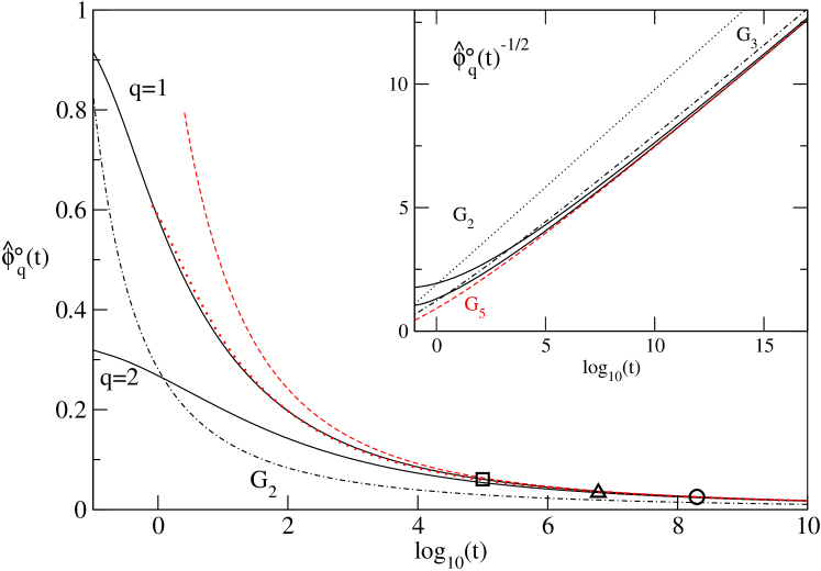
Figure 4: Critical decay at the $A_{3}$-singularity in the two-component model defined by Eqs. (10kpuvaaabamanasauaxbbbca–c) for $v_{3}^{\circ}=45$ and $\tau_{1}=\tau_{2}=1$. The rescaled solutions $\hat{\phi}^{\circ}_{q}(t)=[\phi^{\circ}_{q}(t)-f^{\circ}_{q}]/h_{q}^{\circ}$, $q=1,2$, are shown for as full lines. The asymptotic approximation (10kpuvaaabamanasauaxbba) is shown dashed for $q=1$ and dotted for $q=2$. The points where the approximation deviates by $5\%$ from the solution for $q=1,2$, and the point where the solutions differ by $5\%$ from each other are marked by a square, a triangle and a circle, respectively. The chain curve with label $G_{2}$ shows the leading contribution from Eq. (10kpuvaaabamanasauaxbba). The inset shows as full lines the rectification, $\hat{\phi}^{\circ}_{q}(t)^{-1/2}$ for $q=1$ (lower full line) and $q=2$ (upper full line). The $q$-independent part $G_{5}$ of the approximation in Eq. (10kpuvaaabamanasauaxbba) is given by the dashed line. The dotted and the chain line show the leading and next-to-leading order approximations $G_{2}$ and $G_{3}$, Eq. (10kpuvaaabamanasauaxbba). The time scale $t_{0}$ is $4.07\cdot 10^{-3}$.

Let us use the rescaled correlators $\hat{\phi}_{q}^{\circ}(t)=[\phi^{\circ}_{q}(t)-f^{\circ}_{q}]/h_{q}^{\circ}$ for the following considerations. The result in Eq. (10kpuvaaabamanasauaxbba) assumes the form $\hat{\phi}_{q}^{\circ}(t)=G_{5}(x)+K_{q}^{\circ}\tilde{G}_{5}(x)$, with $G_{5}(x)$ from Eq. (10kpuvaaabae) and $\tilde{G}_{5}(x)=g_{2}^{2}(x)+2g_{2}(x)g_{3}(x)$. Since $\tilde{G}_{5}(x)$ is of higher order than $G_{5}(x)$, Eq. (10kps), correlators for different $q$ approach each other for sufficiently large time as is demonstrated in Fig. 4. The time $t\approx 2\cdot 10^{8}$, where $\hat{\phi}_{2}^{\circ}$ deviates by $5\%$ from $\hat{\phi}_{1}^{\circ}$, is marked by a circle. The amplitude $K_{q}^{\circ}$ introduces the $q$-dependent corrections which are smaller for $q=1$ than for $q=2$. To evaluate $G_{5}(x)$ and $\tilde{G}_{5}(x)$, we determined the following parameters, $\mu_{3}=0.772$, $\kappa=0.888$, and $\mu_{4}=1.38$. Notice, that $\mu_{3}$ is more than twice as for the model studied in Fig. 1. Since the coefficients $c_{m,l}$ in Eq. (10kpuvz) contain powers of $\mu_{3}$ in the denominator, corrections are smaller if $\mu_{3}$ is larger, cf. Eqs. (10kpuvaaa)–(10kpuvaac) and (10kpuvaaab)–(10kpuvaaabd). Because of the smaller corrections, the time scale can be matched with $G_{5}(x)$ between $t=10^{20}$ and $10^{25}$ which is significantly earlier than for the model studied in Fig. 1. We get $t_{0}=4.07\cdot 10^{-3}$.

The asymptotic approximation (10kpuvaaabamanasauaxbba) is shown as a dashed line for $q=1$ in Fig. 4, it deviates by more than $5\%$ from the solution if $t\lesssim 10^{5}$ ($\square$). The approximation for $q=2$ (dotted) deviates by more than $5\%$ for $t\lesssim 6\cdot 10^{6}$ ($\triangle$). This difference in the range of validity can be understood qualitatively by considering the $q$-dependent corrections of higher order in Eq. (10kpuvaaabamanasauaxa), $K_{q}[g_{3}^{2}(x)+2g_{2}(x)g_{4}(x)]+Y_{q}g_{2}^{3}(x)/a_{q}$ with $Y_{q}$ from Eq. (10kpuvaaabamanasauaw). Both $K_{q}$ and $Y_{q}/a_{q}$ are smaller for the first correlator, $Y_{1}/a_{1}=-0.1928$ and $Y_{2}/a_{2}=5.761$, and introduce less deviations from the $q$-independent part $G_{6}(x)$ of the approximation in higher order.

The $q$-independent function $G_{5}(x)$ would lie on top of the dashed line in Fig. 4 and is therefore shown only in the inset which also displays the critical correlators and the $q$-independent functions $G_{2}(x)$ and $G_{3}(x)$, Eq. (10kpuvaaabae). Plotting $\hat{\phi}^{\circ}_{q}(t)^{-1/2}$ we can identify $1/\ln^{2}t$-behavior as straight line. The critical correlators exhibit a straight line starting from $t\approx 10^{9}$. The leading approximation $G_{2}(x)$ is a straight line as well but has a slope slightly larger than the solution. The first correction $G_{3}(x)$ resembles the slope of the solution but is offset from the solution by a shift of the time scale. This was observed before in Fig. 1. Since $G_{5}(x)+K^{\circ}_{q}\tilde{G}_{5}(x)$ was used to match the time scale $t_{0}$ and as $\tilde{G}_{5}(x)$ decays faster than the $q$-independent part, $G_{5}(x)$ coincides with the solution for larger times.

As a second example, the asymptotic laws shall be considered for the square-well system (SWS). This is the microscopic model for a colloid explained in Sec. 1. The microscopic version of MCT for colloids is used with the wave-vector moduli discretized to a set of $M=500$ values. The structure factors that define the mode-coupling functional ${\cal F}_{q}$ in Eq. (1) are calculated in the mean-spherical approximation. We shall consider the same $A_{3}$-singularity for $\delta^{\circ}=0.03$ as considered in previous studies [26, 27]. The reader is referred to these papers for further details and for an extensive discussion of the relaxation near the specified $A_{3}$-singularity. For the evaluation of the approximation (10kpuvaaabamanasauaxbba), we need the correction amplitudes $K^{\circ}_{q}$ which are shown in Fig. 8 of Ref. [26] and the parameters characteristic for the $A_{3}$-singularity under discussion,

$$\mu_{3}=0.109,\,\quad\kappa=0.314\,,\quad\mu_{4}=0.204\,.$$ (10kpuvaaabamanasauaxbbbcbd)

The asymptotic approximation reads

$$\quad\hat{\phi}^{\circ}_{q}(t)=\,60.4/x^{2}+264.7\ln x/x^{3}$$

$$+[3374.9-580.2\ln x+870.4\ln^{2}x]/x^{4}$$

$$+[-11745.7-27952.1\ln x-4452.2\ln^{2}x+2544.1\ln^{3}x]/x^{5}$$

$$+K^{\circ}_{q}\left\{3643.9/x^{4}+31953.7\ln x/x^{5}\right\}+{\cal O}(x^{-6})\,.$$ (10kpuvaaabamanasauaxbbbcbe)

The first line represents $g_{2}(x)$ and $g_{3}(x)$, Eqs. (10kps) and (10kpuvx). The second and third line exhibit the contributions up to $g_{4}(x)$ and $g_{5}(x)$, Eqs. (10kpuvz-10kpuvaaabd), which are independent of the wave vector. The $q$-dependent correction terms appear with the prefactor $K^{\circ}_{q}$ in the curly brackets; they are positive for $t/t_{0}>2.5$ and monotonically decreasing for $t/t_{0}>3.1$.

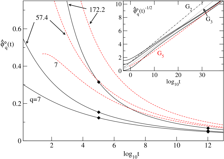
Figure 5: Critical decay at the $A_{3}$-singularity of the square-well system (SWS) for the relative attraction-shell width $\delta^{\circ}=0.03$. Full lines show the rescaled correlation functions $\hat{\phi}^{\circ}_{q}(t)=[\phi^{\circ}_{q}(t)-f_{q}^{\circ}]/h_{q}^{\circ}$ at $\mathbf{V}^{\circ}$, for the wave-vector values $qd=7,\,57.4,$ and $172.2$ as indicated. The unit of time is chosen so that $1/D_{0}=160$, with $D_{0}$ denoting the single particle diffusivity [26, 27]. The dashed lines exhibit the asymptotic approximation of Eq. (5.3) with a time scale $t_{0}=4\cdot 10^{-5}$ matched in the interval $t=10^{40}$…$10^{45}$. For $qd=7.0$, $57.4$, and $qd=172.2$, the correction amplitudes are $K^{\circ}_{q}=-1.704$, $-0.00224$, and $4.814$, respectively. The filled diamonds for $t=10^{5}$ and $t=10^{12}$ mark the values for $\hat{\phi}^{\circ}_{q}(t)$ for the three $q$-values. The inset shows $\hat{\phi}^{\circ}_{q}(t)^{-1/2}$ for the $q$-values above from top to bottom and the $q$-independent approximations defined in Eq. (10kpuvaaabae) in the same representation, $G_{2}(t)^{-1/2}$, $G_{3}(t)^{-1/2}$ and $G_{5}(t)^{-1/2}$, respectively.

Figure 5 shows the rescaled functions $\hat{\phi}^{\circ}_{q}(t)$ for three representative wave numbers. At the peak of the structure factor, $qd=7$, the amplitude is negative, for $qd=57.4$ the correction amplitude is close to zero, and for the wave vector $qd=172.2$ the amplitude is positive. The functions (full lines) deviate strongly from each other in the window of time presented, demonstrating severe violation of the factorization property. If the deviations among the correlation functions for different wave vectors cannot be assigned to the $q$-dependent corrections in Eq. (5.3) within an accessible window in time, we cannot expect that Eq. (5.3) will be sufficient to describe the critical decay. Suppose, the critical correlators for different wave vectors are approximated by Eq. (5.3). Then, for arbitrarily chosen wave vectors $q_{1}$ and $q_{2}$, the difference $\hat{\Delta}[q_{1},q_{2}](t)=\hat{\phi}^{\circ}_{q_{1}}(t)-\hat{\phi}^{\circ}_{q_{2}}(t)$ is given in leading order by the difference in the correction amplitudes, $K^{\circ}_{q_{1}}-K^{\circ}_{q_{2}}$, and the terms in the curly brackets in Eq. (5.3). From Fig. 5 we infer that $\hat{\Delta}[q_{1},q_{2}](t)$ is not yet close to zero to neglect the terms in the curly brackets. The values of $\hat{\phi}^{\circ}_{q}(t)$ for the three chosen $q$-values are marked by diamonds in Fig. 5 for $t=10^{5}$ and $10^{12}$. We get $\hat{\Delta}[7,57.4](10^{5})=-0.030$ and $\hat{\Delta}[172.2,57.4](10^{5})=0.161$. These differences are large but they correctly reflect the ordering in the values for $K^{\circ}_{q}$ which increase with $q$. From that we conclude that the treatment of the $q$-dependence in Eq. (5.3) is qualitatively correct.

If the time dependence of $\hat{\Delta}[q_{1},q_{2}](t)$ were given exclusively by the terms in curly brackets in Eq. (5.3), then the differences among the $K_{q}^{\circ}$ would explain the amplitudes of the decay in $\hat{\Delta}[q_{1},q_{2}](t)$. To quantify deviations from that case we introduce the ratio $\nu[q_{1},q_{2},q_{3}](t)=\hat{\Delta}[q_{1},q_{2}](t)/\hat{\Delta}[q_{2},q_{3}](t)$. For $t\rightarrow\infty$ this ratio is $\nu_{\infty}=(K_{q_{1}}^{\circ}-K_{q_{2}}^{\circ})/(K_{q_{2}}^{\circ}-K_{q_{3}}^{\circ})$. Deviations from $\nu_{\infty}$ indicate that higher-order $q$-dependent corrections are present in addition to the terms in Eq. (5.3). For the $q$-values used in Fig. 5 we get $\nu_{\infty}=(K^{\circ}_{7}-K^{\circ}_{57.4})/(K^{\circ}_{57.4}-K^{\circ}_{172.2})=0.354$. Since $K_{57.4}^{\circ}\approx 0$, this ratio is almost equivalent to $-K^{\circ}_{7}/K^{\circ}_{172.2}$. The ratio at time $t=10^{5}$ is $\nu[7,57.4,172.2](10^{5})=0.187$ and therefore deviates by $90\%$ from $\nu_{\infty}$. Hence, we cannot expect Eq. (5.3) to describe the critical decay in Fig. 5 at that time. At $t=10^{12}$, the ratio has decayed to $\nu[7,57.4,172.2](10^{12})=0.280$ which which deviates from $\nu_{\infty}$ by $20\%$. Here, the $q$-dependent corrections are also in reasonable quantitative agreement with the approximation in Eq. (5.3). To determine $t_{0}$, we use extremely large times. The inset of Fig. 5 displays the rescaled correlators as $\hat{\phi}^{\circ}_{q}(t)^{-1/2}$. In this representation, the leading term $g_{2}(x)$ in Eq. (5) yields a straight line. We see that for large times the correlators for different $q$ indeed come closer together and the ratio at $t=10^{40}$ is $\nu[7,57.4,172.2](10^{40})=0.341$, which deviates by $4\%$ from $\nu_{\infty}$. For the determination of $t_{0}$ we use Eq. (5) for $q=7,\,57.4\,,$ and $172.2$ and match the asymptotic approximation to the numerical solutions in the interval from $t=10^{40}$ to $t=10^{45}$. This results in a value $t_{0}=4\cdot 10^{-5}$. For times larger than $t\approx 10^{50}$ the numerical solution does no longer follow the approximation. In that region inaccuracies in the control-parameter values lead to deviations from the asymptotic behavior. These inaccuracies prevent us also from fixing more than just one digit of $t_{0}$. The dashed line in the inset labeled $G_{5}$ shows the result for neglecting the last line of Eq. (5.3). This also describes the correlator for $q=57.4$ where $K_{q}$ is close to zero. Taking into account only the first line of Eq. (5.3) yields the dotted curve labeled $G_{3}$. This curve is clearly inferior to $G_{5}$, but it captures the slope of the solution still better than $G_{2}$.

In the large panel of Fig. 5, one can compare the critical correlators with the approximation by Eq. (5.3). For times of interest for experimental studies, the description is reasonable qualitatively. Especially the leading $q$-dependent corrections describe the variations seen in the correlators down to relatively short times. The accuracy of the approximation that was demonstrated for the schematic models in Figs. 4 and 1 is far better than seen in Fig. 5 for the SWS. This difference is mainly due to different values of the parameter $\mu_{3}$ that characterizes the various $A_{3}$-singularities. For the two-component model we had $\mu_{3}=0.77$ and for the one-component model there was $\mu_{3}=1/3$. The small value $\mu_{3}=0.109$ for the SWS implies slow convergence of the asymptotic expansion. Therefore, a quantitative description by Eq. (5.3) is possible only for times exceeding considerably the ones shown in Fig. 5.

6 Asymptotic expansion of the critical correlators at an $A_{4}$-singularity

6.1 Expansion up to next-to-leading order

The calculation of the critical correlator at the $A_{4}$-singularity is so involved, that we restrict ourselves to the leading and next-to-leading order result. The Eqs. (10kpuvaaabamana–5.2) remain valid, and Eqs. (10kpuvaaabamanasauaw) and  (5.2) simplify because $\mu_{3}=0$. The difficulty comes about because $\mu_{5}$, which enters Eq. (10kpuvaaabai), has to be determined. This requires the extension of Eq. (10kpuvaaabamanasauaxa), and thereby there appears a further amplitude. The additional amplitude $Z_{q}$ is obtained by also including terms with $n=4$ from Eq. (7). Applying the same manipulations as above, one arrives at $\tilde{\phi}^{\prime\prime}_{q}(t)=Z_{q}\hat{\phi}^{4}+{\cal O}(\hat{\phi}^{5})$ with the amplitude

$$Z_{q}=R_{qk}\{[A_{kk_{1}k_{2}k_{3}k_{4}}^{(4)c}a_{k_{1}}a_{k_{2}}a_{k_{3}}a_{k_{4}}-a_{k}^{4}]+3[A_{kk_{1}k_{2}k_{3}}^{(3)c}a_{k_{1}}a_{k_{2}}X_{k_{3}}-a_{k}^{2}X_{k}]$$

$$+[A_{kk_{1}k_{2}}^{(2)c}X_{k_{1}}X_{k_{2}}-X_{k}^{2}]+2[A_{kk_{1}k_{2}}^{(2)c}a_{k_{1}}Y_{k_{2}}-a_{k}Y_{k}]+\mu_{4}a_{k}^{2}\}\,.$$ (10kpuvaaabamanasauaxbbbcbf)

Introducing the third $q$-dependent correction, the solution assumes the form

$$\hat{\phi}_{q}(t)=a_{q}\hat{\phi}(t)+X_{q}\hat{\phi}^{2}(t)+Y_{q}\hat{\phi}^{3}(t)+Z_{q}\hat{\phi}^{4}(t)+{\cal O}(\hat{\phi}^{5})\,.$$ (10kpuvaaabamanasauaxbbbcbg)

Collecting all terms of order ${\cal O}(\hat{\phi}^{4})$ after including also the line $n=5$ from Eq. (7), one gets from the solvability condition (10kpuvaaabama):

$$\mu_{5}= \sum_{q}\,a^{*}_{q}\{[a_{k}^{5}-A_{kk_{1}k_{2}k_{3}k_{4}k_{5}}^{(5)c}a_{k_{1}}a_{k_{2}}a_{k_{3}}a_{k_{4}}a_{k_{5}}]$$ (10kpuvaaabamanasauaxbbbcbh)

$$+4[a_{k}^{3}X_{k}-A_{kk_{1}k_{2}k_{3}k_{4}}^{(4)c}a_{k_{1}}a_{k_{2}}a_{k_{3}}X_{k_{4}}]$$

$$+3[a_{k}X_{k}^{2}+a_{k}^{2}Y_{k}-A_{kk_{1}k_{2}k_{3}}^{(3)c}(a_{k_{1}}X_{k_{2}}X_{k_{3}}+a_{k_{1}}a_{k_{2}}Y_{k_{3}})]$$

$$+2[X_{k}Y_{k}+a_{k}Z_{k}-A_{kk_{1}k_{2}}^{(2)c}(X_{k_{1}}Y_{k_{2}}+a_{k_{1}}Z_{k_{2}})]\}+\tilde{\kappa}\mu_{4}\,.$$

Summarizing, the asymptotic solution for the critical decay at an $A_{4}$-singularity in next-to-leading order reads

$$\phi_{q}^{*}(t)=f_{q}^{*}+h_{q}^{*}\left\{g_{1}(x)+[g_{2}(x)+K_{q}^{*}g_{1}^{2}(x)]\right\}\,.$$ (10kpuvaaabamanasauaxbbbcbi)

Here, in analogy to Eq. (10kpuvaaabamanasauaxbbb), the critical amplitude is $h_{q}^{*}=(1-f^{*}_{q})a_{q}$ and the correction amplitude is given by $K_{q}^{*}=X_{q}/a_{q}$. The factorization theorem is obeyed by the leading-order term only. Contrary to what was found in Eq. (10kpuvaaabamanasauaxbba) for the behavior at the $A_{3}$-singularity, already the leading correction term $g_{2}$ is modified by the $q$-dependent term $K^{*}_{q}g_{1}^{2}(x)$ of the same order. The higher-order contributions enter the curly brackets in Eq. (10kpuvaaabamanasauaxbbbcbi) as $g_{3}(x)+2g_{1}(x)g_{2}(x)X_{q}/a_{q}+g_{1}^{3}(x)Y_{q}/a_{q}$ and $g_{4}(x)+g_{2}^{2}(x)X_{q}/a_{q}+2g_{1}(x)g_{3}(x)X_{q}/a_{q}+3g_{1}^{2}(x)g_{2}(x)Y_{q}/a_{q}+g_{1}^{4}(x)Z_{q}/a_{q}$. However, $g_{3}(x)$ requires the evaluation of the parameters $\mu_{6}$ and $\kappa^{\prime}$, $g_{4}(x)$ needs $\mu_{7}$ and $\kappa^{\prime\prime}$.

6.2 Discussion

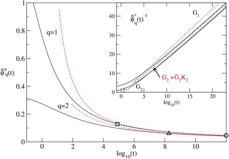
Figure 6: Rescaled critical decay $\hat{\phi}_{q}^{*}=[\phi^{*}_{q}(t)-f_{q}^{*}]/h_{q}^{*}$ at the $A_{4}$-singularity in the two-component model defined in Eqs. (10kpuvaaabamanasauaxbbbca–c) (full lines). The asymptotic approximations, Eq. (10kpuvaaabamanasauaxbbbcbi), for $q=1,2$, are represented by the dashed and dotted curve, respectively. For $q=1$ ($\square$) and $q=2$ ($\triangle$), the points are marked where the solution and the approximation deviate by $5\%$. An additional point is indicated where the solution for $q=2$ differs from the one for $q=1$ by $10\%$ ($\bigcirc$). The inset displays the rectified representation of the solutions for $q=1$ (lower full line) and $q=2$ (upper full line) together with the $q$-independent parts of the approximations, $G_{1}$ and $G_{2}$, cf. Eq. (10kpuvaaabak), and $G_{2}+K_{2}\tilde{G}_{2}$ (see text). The time scale $t_{0}=2.0$ was matched for $t=10^{20}\dots 10^{25}$.

Figure 6 shows the critical decay at the $A_{4}$-singularity of the two-component model defined in Eqs. (10kpuvaaabamanasauaxbbbca–c). The parameters for the evaluation of $g_{1}(x)$ and $g_{2}(x)$ are $\mu_{4}=1.53$, $\mu_{5}=0.962$, and $\kappa=0.386$. We use again the rescaled correlator $\hat{\phi}^{*}_{q}(t)=[\phi^{*}_{q}(t)-f_{q}^{*}]/h_{q}^{*}$ and check first the validity of the factorization in Eq. (10kpuvaaabamanasauaxbbbcbi) in the form $\hat{\phi}^{*}_{q}(t)=G_{2}(x)+K_{q}\tilde{G}_{2}(x)$ where $G_{2}(x)=g_{1}(x)+g_{2}(x)$ and $\tilde{G}_{2}(x)=g_{1}^{2}(x)$. The time, where the solutions for $q=1,\,2$, differ by $5\%$ is only reached at $t\approx 10^{23}$. The circle marks the point where the deviation is still $10\%$ at $t=10^{12}$. We can then use the approximation (10kpuvaaabamanasauaxbbbcbi) to fix the time scale to $t_{0}=2.0$ which then yields the dashed and dotted curves for $q=1,\,2$, accordingly. For $q=1$ this approximation deviates by $5\%$ from the solution at $t\approx 8.2\cdot 10^{4}$ ($\square$). For $q=2$ we find $t\approx 1.8\cdot 10^{8}$ ($\triangle$). This is plausible when appealing to the $q$-dependent higher-order correction in Eq. (10kpuvaaabamanasauaxbbbcbg), which incorporates in addition to drastically different values for $K_{q}$ also the values $Y_{1}/a_{1}=-0.579$ and $Y_{2}/a_{2}=3.76$. A rectified representation of the critical decay and the approximation in the inset shows again the leading-order $G_{1}(x)$ (dotted) as a straight line of different slope than the solution (full lines) and the second correction $G_{2}(x)$ (dashed). In this plot, the critical correlators for different $q$ are still significantly different in the entire window. But Eq. (10kpuvaaabamanasauaxbbbcbi) can account for that difference as is shown by the good agreement of the curve labeled $G_{2}+\tilde{G}_{2}K_{2}$. The latter describes the second correlator where the deviations due to the correction amplitudes are largest.

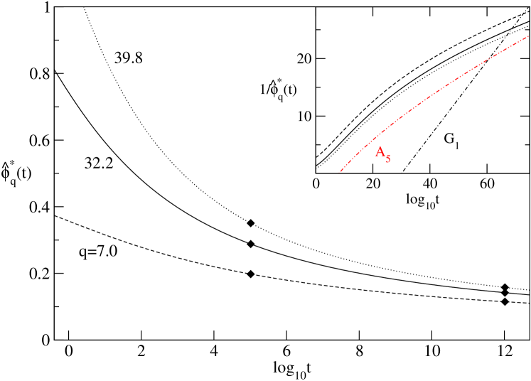
Figure 7: Critical decay at the $A_{4}$-singularity of the SWS for $qd=7.0$ (dashed), $32.2$ (full line), $39.8$ (dotted). The correction amplitudes are $K_{q}=-1.81$, $-0.04$, and $0.77$, respectively. The filled diamonds mark the values at $t=10^{5}$ and $t=10^{12}$ where the ratios $\nu(t)$ are $1.44$ and $1.72$, respectively (see text). The inset replots the curves from the full panel in the same linestyle and shows the first term of Eq. (10kpuvaaabamanasauaxbbbcbk) labeled $G_{1}$ and the law $\ln(t/\tau)^{-2/3}$ labeled $A_{5}$, both with an arbitrary time scale.

We now turn to the $A_{4}$-singularity of the SWS. For the application of Eq. (10kpuvaaabamanasauaxbbbcbi) we need the parameters characterizing the $A_{4}$-singularity,

$$\mu_{4}=0.131\,,\quad\kappa=0.243\,,\quad\mu_{5}=1.21\,.$$ (10kpuvaaabamanasauaxbbbcbj)

The rather small value of $\mu_{4}$ generates particularly large coefficients in the expansion of the critical decay in Eq. (10kpuvaaabaj) where $\mu_{4}$ appears in the denominators. This feature is quite the same as mentioned above for the $A_{3}$-singularities. The asymptotic approximation in Eq. (10kpuvaaabamanasauaxbbbcbi) yields for the critical decay of the rescaled correlators:

$$\qquad\hat{\phi}_{q}^{*}(t)=\;3.54/x-50.7\ln x/x^{2}+12.5\,K_{q}^{*}/x^{2}+{\cal O}(x^{-3})\,.$$ (10kpuvaaabamanasauaxbbbcbk)

We chose again values for $q$ where $K^{*}_{q}$ is negative, almost zero and positive. Figure 7 demonstrates that the factorization is strongly violated. Comparing the solutions $\hat{\phi}_{q}^{*}(t)$ for $t=10^{5}$ we find a ratio defined as in the previous section of $\nu[7,32.2,39.8](10^{5})=1.439$ which is more than $30\%$ off the ratio for the correction amplitudes $\nu_{\infty}=2.185$. At $t=10^{12}$ we find $\nu[7,32.2,39.8](10^{12})=1.723$ which achieves $20\%$ accuracy. So the critical decay at the $A_{4}$-singularity shown in Fig. 7 is in qualitative accord with Eq. (10kpuvaaabamanasauaxbbbcbk) with respect to the variation in $q$. However, due to the small value of $\mu_{4}$, the differences among the correlators for different $q$ do not decay fast enough to allow for a consistent determination of $t_{0}$ for the maximum value in time that could be reached. Numerically we find $\nu[7,32.2,39.8](10^{128})=2.076$ which is still $5\%$ off from $\nu_{\infty}$, and $\hat{\phi}^{*}_{q}(t)$ itself deviates from zero by $5\%$. This illustrates drastically the enormous stretching at the $A_{4}$-singularity.

The inset of Fig. 7 demonstrates that the critical decay $\hat{\phi}^{*}_{q}(t)$ is qualitatively different from the leading order $1/\ln t$-law for $t\leqslant 10^{60}$. For the $A_{3}$-singularity in Fig. 5 it was still possible to argue that curve $G_{2}$ is in accord with the decay qualitatively at least for large times and to attribute deviations for shorter times to the proximity of the $A_{4}$-singularity. Figure 7 does not allow for such an interpretation. The curves $1/\hat{\phi}_{q}^{*}(t)$ have a slope smaller than $1/G_{1}$ over the complete window in time and imply a slower decay than given by the leading order in Eq. (10kpuvaaabamanasauaxbbbcbk). If $\mu_{4}$ was zero, the singularity would be of type $A_{5}$. The leading order critical decay at such butterfly singularity is $\ln(t)^{-2/3}$. This law is added in the inset as chain line labeled $A_{5}$. Indeed, it explains the data qualitatively. Hence, the shortcomings of the asymptotic expansion at the $A_{4}$-singularity in the SWS result from the small value of $\mu_{4}$.

To check if the value for $\mu_{4}$ is exceptionally small for the SWS, the calculation was repeated for the hard-core Yukawa system as introduced in Ref. [16]. We find the even smaller value $\mu_{4}=0.080$. Therefore, the small value of $\mu_{4}$ seems to be typical for systems with short-ranged attraction.

7 Summary

The asymptotic expansion for large times of the critical decay of correlation functions at higher-order glass-transition singularities has been elaborated. These decays can be considered as the analogue of the $t^{-a}$-law expansion for the correlators at the liquid-glass transition. The latter as well as the higher-order singularities are obtained as bifurcations of type $A_{l},\,l\geqslant 2$. The $A_{l}$-singularity and especially the critical decay law at the singularity is characterized by a number $\mu_{l}$. For the $A_{2}$-singularity of the liquid-glass transition, this characteristic number determines the so-called exponent parameter $\lambda=1-\mu_{2}$, which specifies the critical exponent $a$ via $\lambda=\Gamma(1-a)^{2}/\Gamma(1-2a)$. For $\mu_{2}=0$ or $\lambda=1$, one gets $a=0$ and the asymptotic expansion in terms of powers $t^{-a}$ becomes invalid. A higher-order singularity $A_{n}$ is encountered, defined by $\mu_{n}>0$ while $\mu_{l}=0$ for $l<n$.

For an $A_{3}$-singularity, the critical decay is given by an expansion in inverse powers of the logarithm of the time, starting with $1/\ln^{2}t$. The convergence of the asymptotic expansion is the better the larger is $\mu_{3}$. The result for the general models in Eqs. (10kpuvaaabamanasauaxbba) and (10kpuvz) adds probing-variable dependent correction terms to the one-component result. These can be expressed by terms from the one-component solution and correction amplitudes. The leading correction amplitude $K_{q}$ is the same function of the MCT-coupling constants as found earlier for the logarithmic decay-law expansions [24]. Since the vertex is a smooth function of the control parameters, these correction amplitudes are smooth functions as well. Therefore, also for the general case, the range of validity for the asymptotic expansion is determined by the characteristic parameter $\mu_{3}$. If $\mu_{3}$ is small, the quality of the fit by the asymptotic expansion is less satisfactory than for larger $\mu_{3}$. Generically, larger $\mu_{3}$ can be obtained by extending the corresponding glass-glass-transition line deeper into the glassy region and hence having the $A_{3}$-singularity further separated from the liquid regime. Thus, the dynamics influenced by an $A_{3}$-singularity seen in the liquid regime is either connected to a rather small $\mu_{3}$, or it is strongly influenced by a crossing of different liquid-glass-transition lines [27].

For $\mu_{3}=0$, an $A_{4}$-singularity is found; the expansion for one-component models in Eqs. (10kpuvz–10kpuvaaabd,10kpuvaaabae) becomes invalid and has to be replaced by Eqs. (10kpuvaaabaj) and (10kpuvaaabak). The general solution in Eq, (10kpuvaaabamanasauaxbbbcbi) has similar properties as mentioned above for the $A_{3}$-singularity. Now it is the characteristic parameter $\mu_{4}$ that determines how satisfactory the approximation can be. While $\mu_{4}=1$ in Fig. 3 and $\mu_{4}=1.53$ in Fig. 6 allows for a description in the schematic models considered, the small parameter $\mu_{4}\approx 0.1$ in the microscopic models for systems with short-ranged attraction prevents the application of the asymptotic formula.

An understanding of the critical decay law is a prerequisite for estimating the range of validity of the Vogel-Fulcher-type laws which describe the asymptotic limit of the time scale of the logarithmic decay laws near the higher-order singularities [7]. For the two-component model analyzed above, the asymptotic limits were demonstrated for reasonable windows in time [25]. For the mentioned colloid models, the small values of the characteristic parameters $\mu_{3}$ and $\mu_{4}$ together with the manifest violation of the factorization property restrict such laws to unreasonably long times.

References

References

- [1] U. Bengtzelius, W. Götze, and A. Sjölander. Dynamics of supercooled liquids and the glass transition. J. Phys. C, 17:5915–5934, 1984.
- [2] W. Götze. Aspects of structural glass transitions. In J. P. Hansen, D. Levesque, and J. Zinn-Justin, editors, Liquids, Freezing and Glass Transition, volume Session LI (1989) of Les Houches Summer Schools of Theoretical Physics, pages 287–503, Amsterdam, 1991. North Holland.
- [3] W. Götze and L. Sjögren. General properties of certain non-linear integro-differential equations. J. Math. Analysis and Appl., 195:230–250, 1995.
- [4] T. Franosch and Th. Voigtmann. Completely monotone solutions of the mode-coupling theory for mixtures. J. Stat. Phys., 109:237–259, 2002.
- [5] V. I. Arnol’d. Catastrophe Theory. Springer, Berlin, 3rd edition, 1992.
- [6] W. Götze and R. Haussmann. Further phase transition scenarios described by the self consistent current relaxation theory. Z. Phys. B, 72:403–412, 1988.
- [7] W. Götze and L. Sjögren. Logarithmic decay laws in glassy systems. J. Phys.: Condens. Matter, 1:4203–4222, 1989.
- [8] L. Sjögren. Dynamical scaling laws in polymers near the glass transition. J. Phys.: Condens. Matter, 3:5023–5045, 1991.
- [9] S. Flach, W. Götze, and L. Sjögren. The glass transition singularity. Z. Phys. B, 87:29–42, 1992.
- [10] I. C. Halalay. A mode-coupling theory catastrophe scenario description of relaxations in semicrystalline nylons. J. Phys.: Condens. Matter, 8:6157–6173, 1996.
- [11] H. Eliasson. Mode-coupling theory and polynomial fitting functions: A complex-plane representation of dielectric data on polymers. Phys. Rev. E, 64:011802, 2001.
- [12] U. Bengtzelius. Theoretical calculations on liquid-glass transitions in lennard-jones systems. Phys. Rev. A, 33:3433–3439, 1986.
- [13] L. Fabbian, W. Götze, F. Sciortino, P. Tartaglia, and F. Thiery. Ideal glass-glass transitions and logarithmic decay of correlations in a simple system. Phys. Rev. E, 59:R1347–R1350, 1999; 60:2430, 1999.
- [14] J. Bergenholtz and M. Fuchs. Non-ergodicity transitions in colloidal suspensions with attractive interactions. Phys. Rev. E, 59:5706–5715, 1999.
- [15] K. Dawson, G. Foffi, M. Fuchs, W. Götze, F. Sciortino, M. Sperl, P. Tartaglia, Th. Voigtmann, and E. Zaccarelli. Higher order glass-transition singularities in colloidal systems with attractive interactions. Phys. Rev. E, 63:011401, 2001.
- [16] W. Götze and M. Sperl. Higher-order glass-transition singularities in systems with short-ranged attractive potentials. J. Phys.: Condens. Matter, 15:S869–S879, 2003.
- [17] T. Eckert and E. Bartsch. Re-entrant glass transition in a colloid-polymer mixture with depletion attractions. Phys. Rev. Lett., 89:125701, 2002.
- [18] K. N. Pham, A. M. Puertas, J. Bergenholtz, S. U. Egelhaaf, A. Moussaïd, P. N. Pusey, A. B. Schofield, M. E. Cates, M. Fuchs, and W. C. K. Poon. Multiple glassy states in a simple model system. Science, 296:104–106, 2002.
- [19] K. N. Pham, S. U. Egelhaaf, P. N. Pusey, and W. C. K. Poon. Glasses in hard spheres with short-range attraction. Phys. Rev. E, 69:011503, 2004.
- [20] G. Foffi, K. A. Dawson, S. V. Buldyrev, F. Sciortino, E. Zaccarelli, and P. Tartaglia. Evidence for unusual dynamical arrest scenario in short ranged colloidal systems. Phys. Rev. E, 65:050802, 2002.
- [21] E. Zaccarelli, G. Foffi, K. A. Dawson, S. V. Buldyrev, F. Sciortino, and P. Tartaglia. Confirmation of anomalous dynamical arrest in attractive colloids: A molecular dynamics study. Phys. Rev. E, 66:041402, 2002.
- [22] A. M. Puertas, M. Fuchs, and M. E. Cates. Simulation study of non-ergodicity transitions: Gelation in colloidal systems with short range attractions. Phys. Rev. E, 67:031406, 2003.
- [23] F. Mallamace, P. Gambadauro, N. Micali, P. Tartaglia, C. Liao, and S.-H. Chen. Kinetic glass transition in a micellar system with short-range attractive interaction. Phys. Rev. Lett., 84:5431–5434, 2000.
- [24] W. Götze and M. Sperl. Logarithmic relaxation in glass-forming systems. Phys. Rev. E, 66:011405, 2002.
- [25] M. Sperl. Logarithmic decay in a two-component model. In M. Tokuyama, editor, Slow Dynamics in Complex Systems, volume xxx of AIP Conference Proceedings, New York, 2004. AIP.
- [26] M. Sperl. Logarithmic relaxation in a colloidal system. Phys. Rev. E, 68:031405, 2003.
- [27] M. Sperl. Dynamics in colloidal liquids near a crossing of glass- and gel-transition lines. Phys. Rev. E, 69:011401, 2004.
- [28] A. M. Puertas, M. Fuchs, and M. E. Cates. Comparative simulation study of colloidal gels and glasses. Phys. Rev. Lett., 88:098301, 2002.
- [29] F. Sciortino, P. Tartaglia, and E. Zaccarelli. Evidence of a higher-order singularity in dense short-ranged attractive colloids. Phys. Rev. Lett., 91:268301, 2003.
- [30] W. Götze and L. Sjögren. Relaxation processes in supercooled liquids. Rep. Prog. Phys., 55:241–376, 1992.
- [31] W. Feller. An Introduction to Probability Theory and Its Applications, volume II. Wiley & Sons, New York, 2nd edition, 1971.
- [32] M. Abramowitz and I. A. Stegun. Handbook of Mathematical Functions. Dover, New York, 7th edition, 1970.
- [33] M. Sperl. Asymptotic Laws near Higher-Order Glass-Transition Singularities. PhD thesis, TU München, 2003.
- [34] W. Götze and L. Sjögren. A dynamical treatment of the spin glass transition. J. Phys. C, 17:5759–5784, 1984.
- [35] F. R. Gantmacher. The Theory of Matrices, volume II. Chelsea Publishing, New York, 1974.
- [36] J. Bosse and U. Krieger. Relaxation of a simple molten salt near the liquid-glass transition. J. Phys. C, 19:L609–L613, 1987.