Energy barriers in spin glasses

Abstract

For an Ising spin glass on a hierarchical lattice, we show that the energy barrier to be overcome during the flip of a domain of size L scales as $L^{d-1}$ for all dimensions $d$. We do this by investigating appropriate lower bounds to the barrier energy, which can be evaluated using an algorithm that remains fast for large system sizes and dimensions. The asymptotic limit $d\to\infty$ is evaluated analytically.

Energy barriers determine the dynamics of glassy systems that have a complex energy landscape with many metastable states. Typically, the fluctuations between free energy minima in these systems (either between different realizations or in the same random system) scale with observation size $L$ as $L^{\theta}$. It is generally assumed that the free energy barriers encountered in moving from one minimum to another scale with observation size as $L^{\psi}$. However, there exist so far few numerical studies of the value of this exponent in spin glasses, probably because of the difficulty of the problem (in contrast to the many studies of $\theta$). For directed polymers in random systems, the identity $\psi=\theta$ was demonstrated some time ago ourbarrierpapers . For Ising spin glasses, Fisher and Huse derived within the droplet picture the double inequality $\theta\leq\psi\leq d-1$ fisherhuse for dimension $d$. The lower limit is due to the fact that a domain wall has to be introduced into the system if all its spins are to be flipped. However, the minimum domain wall energy scales as $L^{\theta}$. The upper limit is obtained by moving a straight domain wall through the system. Since such a domain wall breaks $L^{d-1}$ bonds, its energy cannot be larger than $\sim L^{d-1}$. Experiments on two- schins93 and three-dimensional jonss02 spin glasses as well as a numerical studies in two dimensions tom91 point towards a value of $\psi$ close to or identical to $d-1$. On the other hand, an equality $\psi=\theta$ is sometimes tacitly assumed, as for instance in a recent publication on spin glass dynamics on the hierarchical lattice sas03 , where the probability for a spin flip on the length scale $L$ is chosen to be a function of the effective coupling strength on this scale, which increases as $L^{\theta}$.

In this paper, we consider the Ising spin glass on an hierarchical lattice and show in fact that $\psi=d-1$ in all dimensions. The Hamiltonian of the system is given by

$$H=-\sum_{\langle ij\rangle}J_{ij}S_{i}S_{j}\,,$$ (1)

where $\langle ij\rangle$ indicates the sum over all nearest-neighbor pairs, and the spins assume the values $\pm 1$. We will mainly consider a Gaussian distribution of couplings with zero mean and unit width. The hierarchical lattice gives for the exponent $\theta$ in dimension $d=2$ the value $-0.27$ BM84 which compares well with the value $-.29$ from recent numerical studies on the square lattice HM while in three dimensions the hierarchical lattice gives $\theta\approx 0.25$ BM84 while on a simple cubic lattice its value is close to $0.20$ AKH99 . Thus the hierarchical lattice provides reasonably good estimates for the value of the exponent $\theta$ (at least for low-dimensional systems) and it is our hope that it is equally useful for determining the value of $\psi$.

The problem of finding energy barriers in glassy systems numerically is usually NP-complete mid99 . We will therefore not attempt to calculate the barrier exactly, but we will rather place bounds on it. Since the upper bound $\psi=d-1$ is already known due to the above-cited argument by Fisher and Huse, we will show in the following that there exists a lower bound to the barrier energy that increases with system size as $L^{d-1}$.

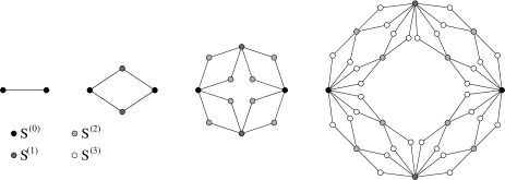
A hierarchical lattice is constructed by starting with one bond connecting two sites. This bond is replaced with a unit consisting of $2^{d-1}$ pairs of bonds, with a new site between each pair. Each of the $2^{d}$ bonds is again replaced with a unit of $2^{d-1}$ pairs of bonds, etc., leading to a lattice with $2^{Id}$ bond after $I$ iterations. In Fig. 1 the first three steps of this process are illustrated for $d=2$.

Figure 1: Iterative construction of the hierarchical lattice. At each step, each bond is replaced with $2^{d-1}$ pairs of bonds, with a new lattice site in between. Different grey shades indicate sites added at different iteration steps.

Evaluating a thermodynamic quantity on the hierarchical lattice with $I$ levels is equivalent to evaluating it on a $d$-dimensional hypercubic lattice of linear size $2^{I}$ using the Migdal-Kadanoff-approximation. Recently, also the dynamics of spin glasses have been studied on hierarchical lattices ric00 ; sas03 ; sch03 , although there is no simple relation to the dynamics on hypercubic lattices. In sas03 ; sch03 , approximations based on renormalization ideas were made.

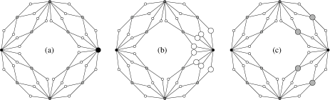
We focus on the energy barrier that has to be overcome when moving from the ground state to the lowest-energy configuration with a domain wall. This domain-wall configuration is obtained by flipping one of the two level-0 spins and by determining the new ground state with this fixed new configuration of the level-0 spins. We allow only single-spin flips when moving from the initial to the final state. At zero temperature (the situation we are considering here), the free-energy barrier is identical to the energy barrier. As indicated above, our goal is to show that there exists a lower bound that scales as $L^{d-1}$. For this purpose, we consider the neighborhood of the right-hand level-0 spin, the “corner spin” (see Fig. 2). We focus our attention on its $L^{d-1}$ level-$I$ nearest neighbors and its $(L/2)^{d-1}$ level-$(I-1)$ next-nearest neighbors. At the moment where the corner spin is flipped, the next-nearest neighbors are in a configuration $\mathcal{C}_{nnn}$. We do not know the configuration of these spins which is associated with the true barrier, but we know that the optimum spin-flip sequence which passes through the true barrier state must have one of the possible configurations $\mathcal{C}_{nnn}$ of the next-nearest neighbor spins at the moment where the corner spin is flipped. Therefore we will later minimize our lower bound with respect to $\mathcal{C}_{nnn}$. We start from the configuration of lowest energy that can be obtained with a given configuration $\mathcal{C}_{nnn}$ of the next nearest neighbors of the right-hand corner spin and with the two corner spins fixed at their initial configuration. Clearly, the energy of this state is at least as high as the energy of the initial configuration. We next calculate the minimum energy barrier that has to be overcome when the right-hand corner spin is flipped with the configuration of the next-nearest neighbors remaining fixed. This minimum energy barrier is obtained by first flipping a suitable selection of the nearest-neighbor spins of the corner spin, before the corner spin itself is flipped. The barrier state is the one immediately before or immediately after the corner spin is flipped, and it is reached from our initial state by spin flips each of which increases the energy. Minimizing the energy barrier (i.e. the energy difference between the barrier state and our initial state) with respect to $\mathcal{C}_{nnn}$ gives a lower bound to the true barrier. This is because the energy of our initial configuration is at least as high as that of the true initial configuration and since the energy of our barrier state cannot be larger than that of the true barrier state.

Figure 2: (a) The right-hand corner site drawn large, (b) its nearest-neighbors drawn large, (c) its next-nearest neighbors drawn large.

In the following, we determine this lower bound to the barrier. The right-hand corner spin is connected to each of its next-nearest neighbors via $2^{d-1}$ intermediate (level-$I$) spins, each of which initially assume the orientation that has the lower energy. Our task now consists in finding those intermediate spins that have to be flipped before the corner spin is flipped, such that the barrier energy is as low as possible. Intermediate spins, for which the absolute value of the coupling to its left neighbor is stronger than the absolute value of the coupling with the corner spin, must not be flipped. This is because for a given configuration of its two neighboring spins, the energy is always lower when the intermediate spin has the orientation that satisfies the left-hand bond and possibly frustrates the right-hand bond. Since the values of the couplings are assigned at random, only about half of the intermediate spins are candidates for being flipped before the corner spin.

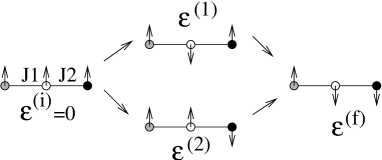
Evaluating all possible combinations of these intermediate spins that might be flipped before the corner spin costs a computer time that increases exponentially with the number of these spins. We will therefore later make an approximation that underestimates the above-defined lower bound to the barrier. In order to define the quantities we need, let us first consider a subunit of three spins (see Fig. 3): The corner spin on the right, one of its next-nearest neighbors to the left of it, and the intermediate spin sitting between the two and connected to both of them. The left-hand spin is fixed. The corner spin is first in its initial configuration. The intermediate spin has the configuration that minimizes the energy. This initial energy is our reference energy, and we set it to zero. Now let $\epsilon^{(1)}$ be the energy of the three-spin unit when the intermediate spin is flipped, and let $\epsilon^{(2)}$ be the energy of the three-spin unit when the right-hand spin (the corner spin) is flipped without first flipping the intermediate spin, and let $\epsilon^{(f)}$ be the energy of the three-spin unit when the right-hand spin is flipped and the intermediate spin is adjusted such that it minimizes the energy. If the left-hand bond is stronger than the right-hand bond, we have $\epsilon^{(2)}=\epsilon^{(f)}$, otherwise we have $\epsilon^{(2)}>\epsilon^{(f)}$.

Figure 3: A subunit of three spins and the energies associated with the different spin configurations mentioned in the text. The figure is drawn for the case that the right-hand bond is stronger than the left-hand bond ($|J2|>|J1|$).

Now let $n$ count all those three-spin units for which the intermediate spin is being flipped before the corner spin, and let $m$ count all those three-spin units for which the intermediate spin is not flipped before the corner spin. The energy of the system just before the corner spin is flipped is

$$\sum_{n}\epsilon_{n}^{(1)}\equiv E_{B}^{(1)}$$

and the energy of the system right after the corner spin is flipped is

$$\sum_{m}\epsilon_{m}^{(2)}+\sum_{n}\epsilon_{n}^{(f)}\equiv E_{B}^{(2)}$$

The lower bound we are looking for is then

$$E_{B} = Min_{C_{nnn}}Min_{n,m}Max\left[E_{B}^{(1)},E_{B}^{(2)}\right]$$ (2)

$$\geq Min_{C_{nnn}}Min_{n,m}\left[\frac{1}{2}(E_{B}^{(1)}+E_{B}^{(2)})\right]$$

$$= Min_{C_{nnn}}Min_{n,m}\left[\frac{1}{2}\left(\sum_{n}(\epsilon_{n}^{(1)}+\epsilon_{n}^{(f)})+\sum_{m}\epsilon_{m}^{(2)}\right)\right]$$

$$= Min_{C_{nnn}}\frac{1}{2}\sum_{i}Min\left[\epsilon_{i}^{(1)}+\epsilon_{i}^{(f)},\epsilon_{i}^{(2)}\right]\equiv S\,.$$

Figure 4: $E_{bub}/2^{d-1}$ as function of dimension $d$. The dashed horizontal line indicates the analytically determined asymptotic value 0.3305 which is approached in the limit $d\to\infty$.

Since $S$ underestimates $E_{B}$, it is also a lower bound to the barrier, and we focus on it in the following. We now perform the minimization with respect to the configuration of the next-nearest neighbor spins, $\mathcal{C}_{nnn}$. For each “bubble” consisting of the corner spin, a next-nearest neighbor and $2^{d-1}$ intermediate spins, the contribution to the above sum is minimized if the next-nearest neighbor is in the configuration that leads to the higher initial bubble energy. We are interested in the average of the above sum over many different systems. Since the contributions of the bubbles to this average are additive, it is sufficient to take the average over one bubble, and our lower bond $S$ is then for large $L$ simply the number of bubbles, $(L/2)^{d-1}$, times this average. The lower bound to the barrier is therefore for large $L$ given by

$$S=(L/2)^{d-1}\times E_{bub}\sim L^{d-1}\,$$ (3)

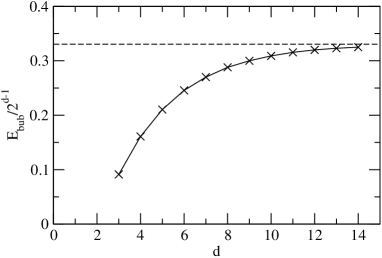
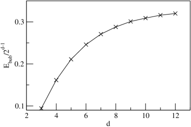
i.e., it scales as $L^{d-1}$. For a Gaussian distribution of unit width of the couplings, the bubble average has in three dimensions the value $E_{bub}=0.364$, i.e. it is positive. It increases with increasing dimension and approaches for large dimensions the asymptotic value $E_{bub}=0.3305\times 2^{d-1}$ (see Fig. 4).

For the limit $d\to\infty$ we can prove analytically that $E_{bub}$ is positive. For each three-spin unit, we call the weaker coupling $J1$, and the stronger coupling $J2$. In the limit $d\to\infty$, one quarter of all three-spin units are initially not frustrated and have the stronger bond on the left-hand side. They make together a contribution $2^{d-3}\langle|J1|\rangle$ to $E_{bub}$. One quarter of all three-spin units are initially not frustrated and have the weaker bond on the left-hand side. They make together a contribution $2^{d-3}\langle|J2|\rangle$ to $E_{bub}$. One quarter of all three-spin units are initially frustrated in the right-hand bond and make together a contribution $-2^{d-3}\langle|J1|\rangle$ to $E_{bub}$. The last quarter of all three-spin units are initially frustrated in the left-hand bond and make together a contribution $2^{d-3}\langle|J2|-2|J1|\rangle$ to $E_{bub}$. Together this gives $E_{bub}=2^{d-2}\langle|J2|-|J1|\rangle$, which is positive since $|J2|>|J1|$. For a Gaussian bond distribution of unit width, $|J1|=2\frac{\sqrt{2}-1}{\sqrt{\pi}}=0.467$ and $|J2|=\frac{2}{\sqrt{\pi}}=1.128$, leading to $E_{bub}=0.3305\times 2^{d-1}$, in agreement with our asymptotic limit in Fig. 4.

Our lower bound $S$ obtained by calculation (2) is negative for $d=2$ and is therefore useless in this case. The reason is that the value of $\epsilon^{(2)}$ is more often negative in $d=2$ than in higher dimensions (because we start from the higher initial bubble energy), leading to a large difference between $E_{B}^{(1)}$ and $E_{B}^{(2)}$ and making the inequality in the second line of (2) worse than in higher dimensions. In order to obtain a positive $E_{bub}$ also in $d=2$, we replace in the second line of (2) the term $\frac{1}{2}(E_{B}^{(1)}+E_{B}^{(2)})$ with the more general expression $aE_{B}^{(1)}+(1-a)E_{B}^{(2)}$, which is valid for all $0<a<1$. We then obtain

$$S=Min_{C_{nnn}}\sum_{i}Min\left[a\epsilon_{i}^{(1)}+(1-a)\epsilon_{i}^{(f)},(1-a)\epsilon_{i}^{(2)}\right]\,.$$

Choosing $a>0.5$ places more weight on the larger energy $E_{B}^{(1)}$ and makes $E_{bub}$ indeed positive. Already for $a=0.51$ we obtain a positive $E_{bub}/2\simeq 0.0039$, and for $a=0.74$, it is as large as 0.12. In $d=1$, the barrier energy is twice the absolute value of the largest bond, which increases as $\sqrt{\ln L}$ for a Gaussian distribution of bonds. We therefore obtain (apart from logarithmic corrections in $d=1$) the general result that the barrier scales on the hierarchical lattice for all $d$ as $L^{d-1}$, implying $\psi=d-1$.

In the following, we argue that our results can be generalized to other bond distributions. For some distributions, our expression for $E_{bub}$ can become negative. This happens for instance for the $\pm J$ model, where the final state of the bubble can be reached from the initial state without first increasing the energy ($E_{bub}=-1.5$ for $d=3$). In this case we modify our calculation in the following way: we first perform a sufficient amount of decimation steps on the hierarchical lattice, until the distribution of the renormalized bonds is such that our expression $S$ (Eq. (2)) for the lower bound becomes positive. It must eventually become positive since the asymptotic bond distribution (if rescaled to unit width) is for all distributions with finite moments the same and is very close to a Gaussian distribution. Then our argument can be repeated on the coarse-grained lattice, giving a new lower bound to the barrier energy for the original lattice. This is because the energy of the system with a given configuration of those spins that survived the renormalization procedure can never be smaller than that of the renormalized system. It turned out that performing one decimation step is sufficient for the $\pm J$ model even in $d=3$ in order to obtain a positive value of $E_{bub}$. Fig. 5 shows $E_{bub}/2^{d-1}$ as function of $d$ for the distribution of bonds that is obtained after one decimation step for bond values $J=\pm 2^{(1-d)/2}$. (The values are chose such that the width of the distribution after one decimation step is 1.) The data are almost indistinguishable from those of Fig. 4. This is to be expected in higher dimensions, since the bond distribution after one decimation step is a binomial distribution, which approaches a Gaussian in high dimensions.

Figure 5: The figure shows a plot of $E_{bub}/2^{d-1}$ for a $J=\pm 2^{(1-d)/2}$ bond distribution after one decimation step as function of dimension $d$.

We therefore obtain even for the $\pm J$ system a lower bound to the barrier that scales as $L^{d-1}$. However, we can expect strong finite-size effects for small system sizes.

To conclude, we have shown that the energy barrier that has to be overcome when introducing a domain wall into an Ising spin glass on a hierarchical lattice scales in all dimensions as $L^{d-1}$, for all bond distributions with finite moments. It remains to be seen if these results can be generalized to conventional lattices. However, we find it encouraging that the experimental data for $\psi$ seem strongly to favor a value close to $d-1$ rather than the “rival”value $\theta$. Since experimental results on spin glasses are not always probing droplets on the length scales at which droplet scaling ideas can be expected to apply without the use of corrections to scaling HM , it is unrealistic to expect perfect agreement for the value of the exponent $\psi$. A further complication is that experimental and numerical data are often studied at temperatures quite close to the transition temperature $T_{c}$, when crossover to critical behavior will also complicate the analysis MBD .