Power laws in surface physics:
The deep, the shallow and the useful

Abstract

The growth and dynamics of solid surfaces displays a multitude of power law relationships, which are often associated with geometric self-similarity. In many cases the mechanisms behind these power laws are comparatively trivial, and require little more than dimensional analysis for their derivation. The information of interest to surface physicists then resides in the prefactors. This point will be illustrated by recent experimental and theoretical work on the growth-induced roughening of thin films and step fluctuations on vicinal surfaces. The conventional distinction between trivial and nontrivial power laws will be critically examined in general, and specifically in the context of persistence of step fluctuations.

Empirical science is apt to cloud the sight, and, by the very knowledge of functions and processes, to bereave the student of the manly contemplation of the whole. The savant becomes unpoetic. Ralph Waldo Emerson

Per Bak’s theory of self-organized criticality is based on the observation that power laws are ubiquitous in nature, and the understanding that this observation requires a (general) scientific explanation. The latter point is often taken for granted in statistical physics, but it is less self-evident in other disciplines. In fact, it could be argued that the predelection of statistical physicists for power law relationships is a professional deformation, which originates in the success story of the theory of equilibrium critical phenomena. In that context, power laws are indeed anomalies which require the ingenious machinery of the renormalization group for their explanation.

However, not every power law carries a deep message. Statistical physicists account for this by distinguishing between trivial and nontrivial power laws. Though deeply rooted in our jargon, this distinction hard to make precise. Most people would agree that the relation

$$\langle\Delta x^{2}\rangle\sim t$$ (1)

for the mean square displacement of a random walker (really a manifestation of the central limit theorem) is a trivial power law, whereas, say, the Onsager exponents for the two-dimensional Ising model are nontrivial. But consider Kolmogorov’s 1941 theory of fully developed turbulence [1]. The derivation of the $k^{-5/3}$-energy spectrum is trivial, in the sense that it uses only dimensional analysis, but it requires the higly nontrivial physical insight that energy dissipation is constant across scales. Clearly the demarcation line between the trivial and the nontrivial also evolves with the progress of science.

Since the discovery of the fractal nature of diffusion-limited aggregation (DLA) more than two decades ago [2], scaling concepts have become one of the main tools in the study of growth processes in condensed matter [3, 4, 5, 6]. While much of the theoretical activity has been driven by the (still unfinished) quest of understanding the two most prominent nontrivial power laws in the field – the fractal dimension of DLA, and the strong coupling exponents of the Kardar-Parisi-Zhang (KPZ) equation [7] in dimensions larger than one [4, 8, 9] – experimentalists have begun to routinely employ the concepts of scaling and self-similarity to analyse topographic data in thin film and crystal growth. In the following I will describe some recent applications of scaling ideas in surface physics. I will argue that, more often than not, power laws that, by the standards of statistical physicists, are quite trivial, have been of most use in interpreting experimental data and gaining insight into kinetic processes at real surfaces. The discussion will include the currently popular concept of persistence of a stochastic process [10], which provides an interesting perspective on the distinction between trivial and nontrivial power laws.

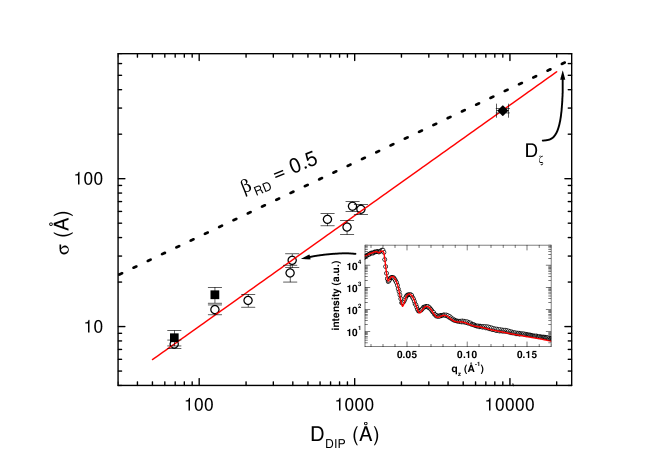
Figure 1: Experimental data for the surface roughenss $\sigma$ as a function of DIP film thickness. Full data points were obtained from atomic force microscopy, and open data points from x-ray diffraction. Inset shows a typical fit of the measured scattering intensity to the form expected for a rough surface (from [11])

Our first example is the growth-induced roughening of thin films of an organic semiconductor, diindenoperylene (DIP) [11]. The relevant scaling law is the relationship between the root mean square surface roughness $\sigma$ (the standard deviation of the film height distribution) and the film thickness $D$,

$$\sigma(D)\sim D^{\beta},$$ (2)

which defines the roughening exponent $\beta$. The experimental data for $\sigma(D)$ shown in Fig.1 are remarkable in several respects. First, they cover more than two decades in film thickness, and they contain consistent results obtained using two completely different methods, x-ray diffraction and atomic force microscopy. The second remarkable feature is the experimentally determined value $\beta=0.75\pm 0.05$ of the roughening exponent. This value exceeds the random deposition (RD) limit $\beta_{\mathrm{RD}}=1/2$, which applies in the absence of any mass transport between different layers of the growing film [3, 6]. In this limit the height follows a Poisson distribution, and (2) becomes equivalent to the random walk relation (1). Random deposition can be approximately realized in the growth of crystalline metal films, where transport between atomic layers is inhibited by step edge barriers (see below). Since mass transport processes along the growing surface are driven by differences in bonding energy, they will generally tend to smoothen the film. The random deposition roughness $\sigma_{\mathrm{RD}}$ would therefore be expected to define an upper bound on the roughness that random fluctuations can induce during the growth of a thin film; in particular, $\beta\leq\beta_{\mathrm{RD}}=1/2$. In this sense systems with $\beta>1/2$ are anomalous, and constitute examples for the (largely unexplained) phenomenon of rapid roughening [4, 11].

But do the DIP data in Fig.1 really violate the RD bound? To answer this question, it is essential to include also the prefactor of the power law relationship (2) in the analysis. Denoting by $d$ the thickness of a single atomic layer, the random deposition roughness is $\sigma_{\mathrm{RD}}=d\sqrt{D/d}$, which is depicted as a dotted line in Fig.1. The comparison shows that the experimental roughness data remain below the random deposition limit even for the largest film thicknesses. It is conceivable (though perhaps not very likely) that the roughening exponent crosses over to a value below 1/2 before the critical thickness $D_{\zeta}$ in Fig.1 is reached, and that the early time value $\beta\approx 0.75$ is merely a transient; unfortunately films with thicknesses $D>D_{\zeta}$ could not be grown for technical reasons. If, on the other hand, the measured value $\beta\approx 0.75$ is truly asymptotic, then the observed roughness cannot be due to the random fluctuations in the deposition beam. In [11] it was conjectured that quenched in-plane disorder arising from the boundaries of the tilt domains in the organic thin film could be responsible for the rapid roughening behavior. Such disorder is known to induce sublinear roughening behavior of the form $\sigma\sim D/\ln(D)^{\psi}$, which can mimic a power law with exponent $1/2<\beta<1$ over extended time scales [13]. Unfortunately, the available experimental information about the growth process on the molecular level is insufficient at present to validate or refute this hypothesis.

If our understanding of DIP film growth, as described above, seems unsatisfactory, it is nevertheless fairly representative of the field as a whole. Although the power law relationship (2) has been, and is currently being reported for a host of growth systems [3, 5], including metallic as well as semiconductor materials and crystalline as well as amorphous films, and although the measured values of $\beta$ tend to cluster around numbers that can be derived from theoretical models [14], a clear-cut example, where a well-understood growth mechanism gives rise to a definite prediction for $\beta$ which is quantitatively confirmed by experiment, is so far missing. In particular, 2+1–dimensional KPZ scaling, a mathematical object under passionate theoretical pursuit for close to twenty years, is still to emerge in any real growth system.

Perhaps the only exception to this statement is mound formation in homoepitaxial crystal growth [6], where the exponent $\beta$ describes the roughening of a morphology that, rather than being scale-invariant, displays a distinct lateral length scale. The growth of “wedding cakes” under conditions of strongly inhibited interlayer transport is particularly simple [16, 17]. In this limit the roughening exponent takes on the random deposition value $\beta=\beta_{\mathrm{RD}}=1/2$, while deviations of the height distribution from the ideal Poisson form show up in the prefactor. The Poisson distribution is cut off at large heights because a new layer can be nucleated on top of a mound only when the top terrace has reached a critical size [18]. This leads to the expression

$$\sigma/d=\sqrt{(1-\theta_{c})D/d}$$ (3)

for the surface roughness, where $\theta_{c}$ is the coverage corresponding to the critical top terrace size [19]. Equation (3) is our first example of a trivial power law where the nontrivial information (the specifics of the interlayer transport processes that determine $\theta_{c}$ [18, 19]) resides in the prefactor.

In the remainder of the paper we will be concerned with the roughening of one-dimensional objects (lines). Rough lines appear naturally as atomic steps on vicinal crystal surfaces [20, 21]. A vicinal surface is obtained by cutting the crystal in a direction close to (in the vicinity of) a high symmetry plane, and it consists of high symmetry terraces separated by steps of monoatomic height. In thermal equilibrium, the steps are roughened by thermal fluctuations. We describe the step at time $t$ by a function $y(x,t)$, where the $x$-axis is taken along the mean step direction and the $y$-direction is perpendicular to the step (in the direction of vicinality). Up to the length scale where collisions with neighboring steps become important the static step conformation is the graph of a one-dimensional random walk, $\langle(y(x,t)-y(x^{\prime},t))^{2}\rangle\sim|x-x^{\prime}|$. Time-dependent fluctuations are well described by a linear Langevin equation of the form

$$\frac{\partial}{\partial t}y(x,t)=-K\left(-\frac{\partial^{2}}{\partial x^{2}}\right)^{z/2}y(x,t)+\eta(x,t)$$ (4)

where $K$ is a positive constant, $\eta(x,t)$ is white noise, and the dynamic exponent $z$ depends on the dominant kinetic pathway through which the step fluctuations relax to equilibrium. The most important cases are $z=2$, corresponding to fast mass exchange between the step and the terrace (nonconserved kinetics) and $z=4$ corresponding to mass transport only along the step (conserved kinetics). It is straightforward to show from (4) that the temporal step correlations scale as

$$C(t)=\langle(y(x,s)-y(x,s+t))^{2}\rangle\sim t^{1/z}.$$ (5)

By analogy with (2) we can say that the roughening exponent of the step is $\beta=1/2z$.

The scaling law (5) has been observed in many experiments, on both metal and semiconductor surfaces [20, 21]. The focus in these experiments has usually not been on the power laws as such, which (in the sense of our introductory discussion) are rather trivial manifestations of the simple linear dynamics (4). The relation (5) is useful mainly as a classification tool, which serves to identify the dominant step relaxation processes. The nontrivial (and materials-specific) information lies instead in the temperature dependence of the prefactor, which gives insight into the energy barriers governing the atomic processes at the step edge. Examples of such processes are shown in the left panel of Fig.2. The right panel shows simulation data for the correlation function $C(t)$, which illustrate the decrease of the prefactor of the $t^{1/4}$-law as the kink rounding barrier $E_{\mathrm{kr}}$ is increased. As shown by the detailed analysis in [22], the activation energy of the prefactor depends linearly on $E_{\mathrm{kr}}$, provided this quantity is larger than the kink energy (the energy cost for the formation of a kink), and therefore a temperature-dependent measurement of $C(t)$ can be used to experimentally determine $E_{\mathrm{kr}}$.

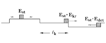
Figure 2: Left panel: Schematic of atomic processes at a step edge. The diffusion of single atoms along straight segments of the step is governed by an energy barrier $E_{\mathrm{st}}$. The detachment from a kink requires the additional energy $E_{\mathrm{det}}$, and the rounding of the kink the energy $E_{\mathrm{kr}}$. The distance between kinks is $\ell_{\mathrm{k}}$. Right panel: Temporal step correlation function $C(t)$ obtained from Monte Carlo simulations for different values of $E_{\mathrm{kr}}$. Dashed lines are fits of the form $C(t)=At^{1/4}$ (from [22])

It would be premature to conclude, however, that the kinetics of step fluctuations can be reduced completely to “trivial” power laws like (5). Although the Langevin equation (4) is linear, it is still considerably more complex than a simple random walk, because the step is a spatially extended object. As a consequence, the step position $y(x,t)$ at fixed $x$ is a non-Markovian process in $t$. The non-Markovian character of a stochastic process manifests itself clearly when considering the persistence probability, i.e. the probability that the process does not cross a particular value in a specified time interval. The computation of this quantity requires the knowledge of temporal correlations of arbitrary order. For a Gaussian process, such as the solution of the Langevin equation (4), all higher order correlation functions are, in principle, encoded in the two-point function (5), but in practice the calculation of the persistence probability for a general Gaussian process is a hard, unsolved problem [10].

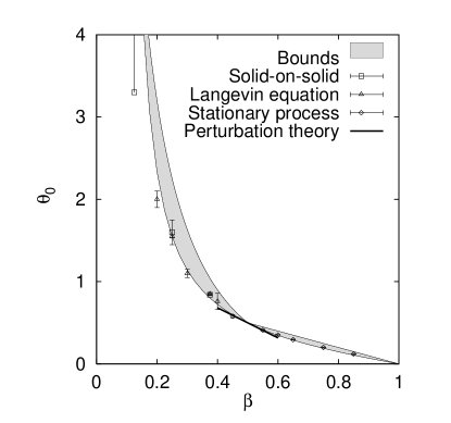
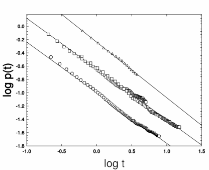
Figure 3: Left panel: Transient persistence exponent $\theta_{0}$ as a function of the roughening exponent $\beta$ for the linear Langevin equation (4). The figure shows numerical estimates obtained from discrete solid-on-solid models (squares), direct simulation of the Langevin equation (triangles), simulation of an equivalent stationary Gaussian process (diamonds), a perturbation expansion around the Markovian case $\beta=1/2$ (bold line) and rigorous bounds derived by comparison with related Markovian processes (gray area) (from [23]). Right panel: Experimentally determined persistence probability for steps on a Si(111)-surface which has undergone a reconstruction by deposition of a fraction of a monolayer of Al. Symbols show measurements at 970 K (squares), 870 K (circles) and 770 K (triangles). The data sets have been shifted vertically for greater clarity; in fact the data show no systematic temperature dependence (from [28])

To be concrete, we define the step persistence probability

$$P(t_{0},t)=\mathrm{Prob}[y(s)\neq y(t_{0})|t_{0}\leq s\leq t_{0}+t],$$ (6)

where it is understood that the step is completly straight at time $t=0$ ($y(x,0)\equiv 0$). Note that here the specified level that the step should not cross is set by its position at the beginning of the time interval. The analytic and numerical investigations in [23] have shown that the quantity (6) displays two distinct scaling regimes. In the transient regime $t_{0}\ll t$ the persistence probability decays as $P\sim t^{-\theta_{0}}$, while in the steady state regime $t_{0}\gg t$ it decays as $P\sim t^{-\theta_{S}}$. The two persistence exponents $\theta_{0}$ and $\theta_{S}$ are different. Moreover, while the steady state exponent is simply related to the roughening exponent $\beta$ by

$$\theta_{S}=1-\beta,$$ (7)

the transient exponent is truly “nontrivial”, in the sense that it can be computed only approximately using a range of fairly sophisticated methods (see Fig.3).

The relationship (7) provides a good illustration of the fallibility of the distinction between trivial and nontrivial scaling exponents. On the one hand it would seem that $\theta_{S}$, being simply related to the arguably trivial exponent $\beta$, should also be classified as trivial. On the other hand the relation (7), while well supported by simulations and plausible scaling arguments, is not rigorously established; in fact, in the context of the general problem of determining the persistence probability of a Gaussian process with known correlator, there is no reason why $\theta_{S}$ should be simpler to compute, and hence less nontrivial, than $\theta_{0}$. The scaling relation (7) holds because the stochastic process $y(x,t)$ at fixed $x$, in the steady state regime, combines two invariance properties: It is scale invariant as well as translationally invariant in time[26]. Because it is based on these general principles, (7) appears to hold also for non-Gaussian interface fluctuations, such as those of the KPZ universality class, where not even the temporal two-point correlations (let alone correlations of higher order) are explicitly known [27].

Several groups have recently met the challenge of experimentally measuring the persistence probability of one-dimensional interfaces, for steps on vicinal surfaces [28, 29, 30] as well as for slow combustion fronts in paper [31]. In all cases the steady state persistence exponent $\theta_{S}$ was measured, and the scaling relation (7) was confirmed, with $\beta=1/4$ [28], $\beta=1/8$ [29] and $\beta=1/3$ [31], respectively. The transient persistence exponent (which is of greater theoretical interest) has so far not been experimentally accessible, because of the difficulty of preparing the special (flat) initial condition that it refers to. In addition to the persistence probability defined by (6), in [28] also the probability for the step not to cross the mean step position (determined as an average over the measured time series) was considered. This quantity turns out not to follow a power law. This is because in the thermodynamic limit the step position starts, with probability one, infinitely far away from the mean (the variance of $y$ diverges with diverging step length); hence the persistence probability remains at unity and decays exponentially only on a much larger time scale set by the finite length of the step [32, 33].

Experimental step persistence data from [28] are displayed in the right panel of Fig.3. In contrast to the step correlation function in Fig. 2, the persistence data show no systematic temperature dependence; the prefactor of the observed power law depends only on the sampling time [34]. This is because the property of a height fluctuation to return (or not) to its initial value in a prescribed time interval does not depend on the overall amplitude of the fluctuation; the persistence probability is a functional only of the shape of the (suitably normalized) correlation function [16]. As a consequence, persistence measurements cannot be used to extract energy barriers for specific microscopic processes. The benefit of these measurements is of a more fundamental nature – they prove that the theoretical description of step fluctuations through the Langevin equation (4), and the underlying picture of “universality classes” encoded by the dynamic exponent $z$, extends beyond the two-point function to correlations of arbitrary order. As the persistence probability is known to be extremely sensitive to hidden temporal correlations affecting the interface fluctuations [27], it may be particularly useful in cases where the assignment of the universality class (the value of $z$) through more conventional measurements is ambiguous.

Where does this leave us with regard to the general reflections on power laws, the trivial and the nontrivial, the deep and the shallow, which introduced this paper? From discussions in the early 1990’s, when SOC was challenged by the competing concept of Generic Scale Invariance [36], I recall that Per Bak had a distinct, and rather unfavorable opinion of simple power laws generated by simple equations such as (4): He referred to them as systems operating by the garbage in, garbage out principle, because they merely perform a (linear, or, more generally, nonlinear) transformation of the driving white noise into correlated fluctuations. Per viewed self-organization as an essential part of SOC. He emphasized the capability of self-organizing systems to develop new, emergent levels of structure, and to undergo a history which is open to contingent influences. Is a rough surface or a fractal cluster grown by DLA self-organized in this sense? Probably not. Still, we must accept that many of the power laws in the world that surrounds us have rather humble origins. As theoretical physicists, our task it to explain these origins; but as “experimental philosophers” (Per Bak) we would also like to know what they mean. The latter question is of course not one to be answered, but one that is to be constantly clarified (and reobscured) in the ongoing discourse of the community. In these discussions Per will be sorely missed, and gratefully remembered for a long time to come.

References

- [1] U. Frisch: Turbulence (Cambridge University Press, 1995)
- [2] T.A. Witten, L.M. Sander: Phys. Rev. Lett. 47, 1400 (1981)
- [3] A.–L. Barabàsi, H.E. Stanley: Fractal Concepts in Surface Growth, (Cambridge University Press, 1995)
- [4] J. Krug: Adv. Phys. 46, 139 (1997)
- [5] P. Meakin: Fractals, Scaling and Growth far from Equilibrium (Cambridge University Press, 1998)
- [6] T. Michely and J. Krug, Islands, Mounds and Atoms. Patterns and Processes in Crystal Growth Far from Equilibrium (Springer, Berlin 2003)
- [7] M. Kardar, G. Parisi, Y.-Z. Zhang: Phys. Rev. Lett. 56, 889 (1986)
- [8] J. Krug and H. Spohn, in: Solids far from Equilibrium, ed. by C. Godrèche (Cambridge University Press, Cambridge 1991) pp. 479–582
- [9] T. Halpin-Healy, Y.C. Zhang: Phys. Rep. 254, 215 (1995)
- [10] S.N. Majumdar: Curr. Sci. 77, 370 (1999)
- [11] A.C. Dürr, F. Schreiber, K.A. Ritley, V. Kruppa, J. Krug, H. Dosch, B. Struth: Phys. Rev. Lett. 90, 016104 (2003)
- [12] K.J. Caspersen, A.R. Layson, C.R. Stoldt, V. Fournee, P.A. Thiel, J.W. Evans: Phys. Rev. B 65, 193407 (2002)
- [13] J. Krug: Phys. Rev. Lett. 75, 1795 (1995)
- [14] J. Krim, G. Palasantzas: Int. J. mod. Phys. B 9, 599 (1995)
- [15] J. Maunuksela, M. Myllys, O.-P. Kähkönen, J. Timonen, N. Provatas, M. J. Alava, T. Ala-Nissila: Phys. Rev. Lett. 79, 1515 (1997)
- [16] J. Krug: J. Stat. Phys. 87, 505 (1997)
- [17] M. Kalff, P. Šmilauer, G. Comsa, T. Michely: Surf. Sci. 426, L447 (1999)
- [18] J. Krug, P. Politi, T. Michely: Phys. Rev. B 61, 14037 (2000)
- [19] J. Krug, P. Kuhn, in: Atomistic Aspects of Epitaxial Growth, ed. by M. Kotrla, N.I. Papanicolaou, D.D. Vvedensky, L.T. Wille (Kluwer, Dordrecht 2002) pp. 145–163
- [20] H.-C. Jeong, E.D. Williams: Surf. Sci. Rep. 34, 171 (1999)
- [21] M. Giesen: Prog. Surf. Sci. 68, 1 (2001)
- [22] J. Kallunki, J. Krug: Surf. Sci. Lett. 523, L53 (2003)
- [23] J. Krug, H. Kallabis, S.N. Majumdar, S. Cornell, A.J. Bray, C. Sire: Phys. Rev. E 56, 2792 (1997)
- [24] B.B. Mandelbrot, J.W. van Ness: SIAM Rev. 10, 422 (1968)
- [25] S.N. Majumdar: Phys. Rev. E 68, 050101(R) (2003)
- [26] J. Krug: Markov Proc. Rel. Fields 4, 509 (1998)
- [27] H. Kallabis, J. Krug: Europhys. Lett. 45, 20 (1999)
- [28] D.B. Dougherty, I. Lyubinetsky, E.D. Williams, M. Constantin, C. Dasgupta, S. Das Sarma: Phys. Rev. Lett. 89, 136102 (2002)
- [29] D.B. Dougherty, O. Bondarchuk, M. Degawa, E.D. Williams: Surf. Sci. Lett. 527, L213 (2003)
- [30] M. Constantin, S. Das Sarma, C. Dasgupta, O. Bondarchuk, D.B. Dougherty, E.D. Williams: Phys. Rev. Lett. 91, 086103 (2003)
- [31] J. Merikoski, J. Maunuksela, M. Myllys, J. Timonen: Phys. Rev. Lett. 90, 024501 (2003)
- [32] C. Dasgupta, M. Constantin, S. Das Sarma, S.N. Majumdar: Preprint (cond-mat/0307086)
- [33] S.N. Majumdar (private communication)
- [34] E.D. Williams (private communication)
- [35] D.Avnir, O. Biham, D. Lidar, O. Malcai: Science 279, 39 (1998)
- [36] G. Grinstein, D.-H. Lee, S. Sachdev: Phys. Rev. Lett. 64, 1927 (1990)