The steady state structure of an interface in an Ising system on a square lattice placed in a non-uniform external field, shows a commensurate -incommensurate transition driven by the velocity of the interface. The non-uniform field has a profile with a fixed shape which is designed to stabilize a flat interface, and is translated with velocity $v_{e}$. For small velocities the interface is stuck to the profile and is rippled with a periodicity which may be either commensurate or incommensurate with the lattice parameter of the square lattice. For a general orientation of the profile, the local slope of the interface locks in to one of infinitely many rational directions producing a devil’s staircase structure. These “lock-in” or commensurate structures dissappear as $v_{e}$ increases through a kinetics driven commensurate - incommensurate transition. For large $v_{e}$ the interface becomes detached from the field profile and coarsens with Kardar-Parisi-Zang exponents. The complete phase -diagram and the multifractal spectrum corresponding to these structures have been obtained numerically together with several analytic results concerning the dynamics of the rippled phases. Our work has technological implications in crystal growth and the production of surfaces with various desired surface morphologies.

I Introduction

Commensurate-in -commensurate (C-I) transitionsChaikin have been extensively studied over almost half a century following early experiments on noble gases adsorbed on a crystalline substrateKr eg. Kr on graphite. Depending on coverage and temperature, adsorbates may show high density periodic structures the reciprocal lattice vectors (RLVs) of which are either a rational (commensurate) or irrational (in -commensurate) multiple of a substrate RLV. By changing external parameters (eg. temperature) one may induce phase-transitions between these structures. Recently, the upsurge of interest in the fabrication of nano-devices have meant a renewed interest in this field following a large number of experimental observations on “self-assembled” domain patterns (stripes or droplets) on epitaxially grown thin films for eg. Ag films on Ru(0001) or Cu-Pb films on Cu(111)films etc. The alloy films often show composition modulations in the lateral direction forming patterned superlattices. These self-assembled surface patterns may have potential applications in the field of opto-electronics, hence the interest. In general, the whole area of surface structure modification has tremendous technological implications including, for example, the recording industry where magnetic properties are intimately connectedmagnet to surface structure.

Almost universally, C-I transitions may be understood using some version of the simple Frenkel -KontorovaFK (FK) model, which models them as arising from a competition between the elastic energy associated with the distortion of the adsorbate lattice and substrate -adsorbate interactions. A complicated phase diagram involving an infinity of phases corresponding to various possible commensuration ratios (rational fractions) is obtained as a function of the two energy scales. In-between two commensurate structures one obtains regions where the periodicity of the adsorbate lattice is in -commensurate. All C-I transitions are equilibrium transitions in the sense that at any value of the relevant parameters, the structures observed optimize a free -energy. Indeed, despite its importance, the dynamical aspect of C-I transitions is a relatively unexplored domain.

In this paper, on the other hand, we discuss a C-I transition entirely driven by kinetics. We show that $(1)$ a simple Ising interface in a square lattice, held in place by a non-uniform external magnetic field, can have a variety of commensurate “phases” characterized by the local slope expressed in terms of the unit vectors of the underlying lattice and $(2)$ it is possible to induce transitions in-between these phases by externally driving the interface with the help of the field. The independent variables are therefore the average slope of the interface and its velocity both of which, as we show, can be externally controlled. Preliminary results from this work has been published elsewherephysica ; prl .

The dynamics of a 2-d Ising interface between the “up” and “down” spin phases at low temperature T, in a (square) lattice driven by uniform external fields is a rather well studiedBarabasi ; Maj1 subject. The interface moves with a constant velocity, $v_{\infty}$, which depends on the applied field, $h$ and the orientation $\theta$ measured with respect to the underlying lattice. The interface is rough and coarsens with KPZBarabasi exponents $\alpha=1/2$ and $\beta=1/3$ where $\alpha$ and $\beta$ are the roughness and dynamical exponents respectively. We explore the possibility of driving such an interface with a pre-determined velocity $v_{f}$ using an external non-uniform field which changes sign following a sharp sigmoidal profile forcibly stabilizing a stationary, macroscopically flat interface at the region where the field crosses zero. We study systematically the structure and dynamics of this “forced” Ising interface as the field profile is moved without change of shape at an externally controlable velocity $v_{e}$. We show that for low driving velocities $v_{e}$, the interface velocity $v_{f}=v_{e}$ and the interface is stuck to the profile — the “stuck” phase. For larger $v_{e}>v_{\infty}$, the interface detaches. In the stuck phase the interface, though macroscopically flat (i.e. $\alpha=\beta=0$) is patterned on the scale of the lattice spacing. It is these patterns which we show, undergo a series of C-I transitions determined by the $v_{e}$ and the geometry characterized by the average slope of the interface in terms of the lattice vectors of the underlying square lattice.

In the next section we introduce the model and briefly sketch the main results from a mean field treatment. In section III we map our interface dynamics to the dynamics of a one dimensional “exclusion process” – a system of hard core particles on a line. In section III-A and B we present our results for the ground state structure and the dynamics within this model. Finally, in section IV we conclude.

II THE MODEL AND MEAN FIELD THEORY

Figure 1: (a) An Ising interface $Y(x,t)$ (bold curved line) between regions of positive (marked $+$) and negative (marked $-$) magnetization in an external, inhomogeneous field with a profile which is as shown(dashed line). The positions of the edge of the field profile and that of the interface are labelled $S_{e}$ and $S_{f}$ respectively. (b) A portion of the interface in a square lattice showing a corner. (c) The interface velocity $v_{f}$ as a function of the velocity of the dragging edge $v_{e}$ for $N_{s}=100(\Box),1000(\Diamond),10000(+)$ and $\rho=0.5$. All the data ($\Box,\Diamond,+$) collapse on the mean field solution (dashed line). Inset shows the graphical solution (circled) of the self-consistency equation for $v_{f}$; dashed line represents $v_{f}=v_{f}$.

We consider here (see Fig.1) a one-dimensional interface $Y(x,t)$ between phases with magnetization, $\phi(x,y,t)>0$ and $\phi(x,y,t)<0$, in a 2-d square lattice obeying single-spin flip Glauber dynamics Men in the limit $h/J,T/J\rightarrow 0$. Here $J$ is the Ising exchange coupling and $T$ the temperature. An external non-uniform field is applied such that $h={\it h_{max}}$ in the +ve and $-{\it h_{max}}$ in the -ve $\phi$ regions separated by a sharp edge. The edge of the field (i.e. where the field changes sign) lies at $S_{e}$. The front or interface, $Y(x,t)$, separates up and down spin phases. The interface is the bold curved line (Fig.1) with the average position $S_{f}$. When the edge is displaced with velocity ${\it v_{e}}$; the front,in response, travels with velocity ${\it v_{f}}$. Parts of the front which leads (lags) the edge of the field experience a backward (forward) force pulling it towards the edge. The driving force therefore varies in both space and time and depends on the relative position of the front compared to that of the edge of the dragging field. In the low temperature limit the interface moves solely by random corner flipsBarabasi (Fig. 1(b)), the fluctuations necessary for nucleating islands of the minority phase in any region being absent. We study the behaviour of the front velocity $v_{f}$ and the structure of the interface as a function of $v_{e}$ and orientation.

Naively, one would expect fluctuations of the interfacial coordinate $Y(x,t)$ to be completely suppressed in the presence of a field profile. This expectation, as depicted by our main results (Fig.1, Fig.3 and Fig.5) is only partially true. While, as we show below, a mean field theory gives the exact behaviour of the front velocity $v_{f}$ as a function of $v_{e}$ (Fig.1); small interfacial fluctuations produce a dynamical phase diagram showing infinitely many dynamical phases (Fig 3) and dynamic phase transitions (Fig. 5). For $v_{e}<v_{\infty}$ the interface is stuck to the profile $v_{f}=v_{e}$. The stuck phase has a rich structure showing microscopic, “lock-in”, commensurate ripples. These dissappear at high velocities through a dynamical commensurate- incommensurate (C-I) transition.

Consider, first, a continuum coarse-grained description of the model shown in Fig. 1 . We assume that for $h/J,T/J\rightarrow 0$ the magnetization is uniform everywhere except near the interface, $Y(x,t)$ so that the magenetisation $\phi=\phi(y-Y(x,t))$. The field profile is given by $h(y,t)=h_{max}f(y,t)$ where $f(y,t)=\tanh((y-v_{e}t)/\chi)$ and $\chi$ is the width of the profile (see Fig 1(a)). Using Model A dynamicsChaikin for $\phi$ and integrating out all degrees of freedom except those corresponding to the interfacial position, we obtain the effective dynamical equation satisfied by the interface,

$$\frac{\partial Y}{\partial t}=\lambda_{1}\frac{\partial^{2}Y}{\partial x^{2}}-\lambda_{2}\Big{(}\frac{\partial Y}{\partial x}\Big{)}^{2}f(Y,t)-\lambda_{3}f(Y,t)+\zeta(x,t)$$ (1)

where $\lambda_{1}$,$\lambda_{2}$ and $\lambda_{3}$ are parameters. Note that Eq. (1) lacks Galilean invariancemultif $Y^{\prime}\rightarrow Y+\epsilon x,\>\>x^{\prime}\rightarrow x-\lambda_{2}\epsilon t,\>\>t^{\prime}\rightarrow t$. A mean field calculation amounts to taking $Y\equiv Y(t)$ i.e. neglecting spatial fluctuations of the interface and noise. For large times ($t\rightarrow\infty$), $Y\rightarrow v_{f}t$, where $v_{f}$ is obtained by solving the self-consistency equation;

$$v_{f} = \lim_{t\to\infty}-\lambda_{3}\tanh\Big{(}\frac{(v_{f}-v_{e})t}{\chi}\Big{)}$$ (2)

$$= -\lambda_{3}\,{\rm sign}(v_{f}-v_{e})$$

For small $v_{e}$ the only solution to Eq. (2) is $v_{f}=v_{e}$ and for $v_{e}>v_{\infty}$, where $v_{\infty}=\lambda_{3}$ we get $v_{f}=\lambda_{3}=v_{\infty}$. We thus have a sharp transition  (Fig. 1(c)) from a region where the interface is stuck to the edge to one where it moves with a constant velocity. How is this result altered by including spatial fluctuations of $Y$ ? This question is best answered by mapping the interface problem to an assymmetric exclusion processBarabasi ; AEP and studying the dynamics both analytically and numerically using computer simulations.

III FLUCTUATIONS: THE EXCLUSION PROCESS

The mapping to the exclusion process followsMaj1 ; AEP by distributing $N_{p}$ particles among $N_{s}$ sites of a 1-d lattice. The particles are labelled $i=1,2,.......,N_{p}$ sequentially at $t=0$. Any configuration of the system is specified by the set of integers $\{y_{i}\}$ where $y_{i}$ denotes the location of the $i$th particle. In the interface picture $i$ maps onto a horizontal coordinate ($x$ in Fig. 1), and $y_{i}$ as the local height $Y(x)$. Each configuration $\{y_{i}\}$ defines a one-dimensional interface inclined to the horizontal with mean slope $\tan\theta_{f}=1/\rho$ where $\rho=N_{p}/N_{s}$. The $y_{i}$ satisfy the hard core constraint $y_{i+1}\geq y_{i}+1$. The local slope near particle $i$ is given by $y_{i+1}-y_{i}$ and is equal to the inverse local density $\rho_{i}$ measured in a region around the $i^{\rm th}$ particle. Alternatively, one associates a vertical bond with a particle and a horizontal bond with a holeMaj1 , in which case, again, we obtain an interface with a slope $\tan\theta_{f}^{\prime}=\rho/(1-\rho)$. The two mappings are distinct but equivalent. Periodic boundary conditions amount to setting $y_{i+N_{p}}=y_{i}\pm N_{s}$. Motion of the interface, by corner flips corresponds to the hopping of particles. In each time step ($N_{p}$ attempted hops with particles chosen randomly and sequentiallyAEP ), $y_{i}$ tends to increase (or decrease) by 1 with probability $p$ (or $q$); it actually increses (or decreases) if and only if ${y_{i+1}-y_{i}>1}$. The dynamics involving random sequential updates is known to indroduce the least amount of correlations among $y_{i}$ which enables one to derive exact analytic expressions for dynamical quantities using simple mean field argumentsAEP . The right and left jump probabilities $p$ and $q$ ($p+q=1$) themselves depend on the relative position of the interface $y_{i}$ and the edge of the field profile $i/\rho+v_{e}t$. Note that this relative position is defined in a moving reference frame with velocity $v_{f}(t)$, the instantaneous average particle velocity defined as the total number of particles moving right per time step. We use a bias $\Delta_{i}(t)=p-q=\Delta\,{\rm sign}(y_{i}-i/\rho-v_{e}t)$ with $\Delta=1$ unless otherwise stated. In addition to the front velocity $v_{f}$, we also examine the behaviour of the average position,

$$<y(t)>=N_{p}^{-1}\sum_{i=1,N_{p}}y_{i}(t)$$ (3)

and the width of the interface:

$$\sigma^{2}(t) = N_{p}^{-1}\sum_{i=1,N_{p}}<(y_{i}(t)-<y_{i}(t)>)^{2}>$$ (4)

as a function of time and system size $N_{s}$. Here, $<y_{i}(t)>=i/\rho+v_{e}t$. Angular brackets denotes an average over the realizations of the random noise. Note that the usual particle hole symmetry for an exclusion processBarabasi ; AEP is violated since exchanging particles and holes changes the relative position of the interface compared to the edge.

We perform numerical simulations of the above model for $N_{s}$ upto $10^{4}$ to obtain $v_{f}$ for the steady state interface as a function of $v_{e}$ as shown in Fig. 1(c). A sharp dynamical transition from an initially stuck interface with $v_{f}=v_{e}$ to a free, detached interface with $v_{f}=v_{\infty}=\Delta(1-\rho)$ is clearly evident as predicted by mean field theory. The detached interface coarsens with KPZ exponentsphysica . Note that, even though the mean field solution for $v_{f}(v_{e})$ neglects the fluctuations present in our simulation, it is exact. The detailed nature of the stuck phase ($v_{f}=v_{e}$ and $\sigma$ bounded) is, on the other hand, considerably more complicated than the mean field assumption $Y(x,t)=Y(t)$.

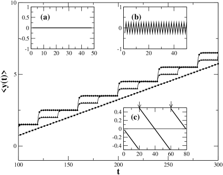
Figure 2: Variation of $<y(t)>$ with $t$ for $v_{e}=0.025$ and $p=1.0$. Lines denote analytic results while points denote Monte Carlo data for $\rho=1/5$ (uppermost curve), $2/5$ and an incommensurate $\rho$ near $1/3$. Inset (a)-(c) shows the corresponding ground state interfaces ($y_{i}-i/\rho$). The arrows in (c) mark the positions of two discommensurations.

III.1 Ground state structure and the Devil’s staircase

The ground state of the interface in the presence of a stationary ($v_{e}=0$) field profile is obtained by minimizing $E=\sum_{i}(y_{i}-i/\rho-c)^{2}$ with respect to the set $\{y_{i}\}$ and $c$. This maybe shown from Eq.(1) by neglecting the terms non-linear in $\partial Y/\partial x$; the resulting equation of motion, for small deviations of $Y$ from the edge may be derived from the effective Hamiltonian $E$. The form of $E$ leads to an infinite range, non-local, repulsive, interaction between particles in addition to hard core repulsion and the minimization is subject to the constraint that $y_{i}$ be an integer. For our system, the result for the energy may be obtained exactly for density $\rho=m/n$, an arbitrary rational fraction. For even m we have the following expression.

$$E = \frac{1}{m}\sum_{j=1,m/2}[(\frac{j}{m}+c)^{2}+(\frac{j}{m}-c)^{2}]+$$ (5)

$$(\frac{1}{2}-c)^{2}+c^{2}$$

$$= \frac{1}{6}(\frac{1}{2}-\frac{1}{m})(1-\frac{1}{m})+\frac{1}{4m}-\frac{1}{4m^{2}}$$

Where in the last equation we have minimized the expression with respect to $c$.

Similarly for odd m we have the following expression for energy,

$$E = \frac{1}{m}\sum_{j=1,m/2-1}[(\frac{j}{m}+c)^{2}+(\frac{j}{m}-c)^{2}]+c^{2}$$ (6)

$$= \frac{1}{12}(1-\frac{1}{m^{2}})$$

The resulting ground state profiles are shown in Fig.  2(insets). The lower bound for $E(\rho)$ is zero which is the energy for all $\rho=1/n$. For irrational $\rho$ the energy is given by $\lim_{m\to\infty}E(m/n)=1/12$ which constitutes an upper bound. For an arbitrary $0\,<\,\rho\,<\,1$ the system ($\{y_{i}\}$) therefore prefers to distort, conforming within local regions, to the nearest low-lying rational slope $1/\tilde{\rho}$ interspersed with “discommensurations” of density $\rho_{d}=|\rho-\tilde{\rho}|$ and sign +ve (-ve) if these regions are shifted towards (away) from each other by $1$. A plot of $\tilde{\rho}(\rho)$ shows a “Devil’s staircase” structureChaikin . In order to observe this in our simulation we analyze the instantaneous distribution of the local density of the particle -hole system to obtain weights for various simple rational fractions. A time average of these weights then give us the most probable density $\tilde{\rho}$ — distinct from the average $\rho$ which is constrained to be the inverse slope of the profile. Increasing the width $\chi$ of the external field profile away from zero gradually washes out this Devil’s staircase structure (Fig. 3).

Figure 3: Devil’s staircase structure in a plot of $\tilde{\rho}$ Vs $\rho$ for small velocities ($v_{e}=0.05$) and $\chi=0.01,1,5$.

As the velocity $v_{e}$ is increased, steps corresponding to ${\tilde{\rho}}=m/n$ (rational fractions) dissappear sequentially for $v_{e}>1/m$ so that for $v_{e}>1/2$ only fractions of the form $1/n$ remain which persist upto $v_{e}=v_{\infty}$. The locus of the discontinuities in the $\tilde{\rho}(\rho)$ curve for various velocities $v_{e}$ gives the phase diagram (Fig. 4) in the $v_{e}-\rho$ plane. Note that the phase diagram for this C-I transition as given in an earlier publicationprl contained inaccuracies which have been now corrected.

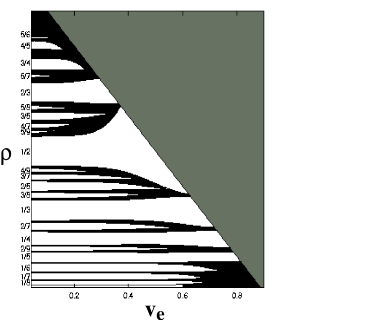
Figure 4: The dynamical phase diagram in $v_{e}$ and $\rho$ plane. The numbers on the $\rho$ axis mark the fractions $\tilde{\rho}$, which determines the orientation of the lock-in phase. The three regions white, black and grey correspond to the rippled, the disordered and the detached phases respectively.

III.2 Dynamics of the forced Interface

For low velocities and density where correlation effects due to the hard core constraint are negligible, the dynamics of the interface may be obtained exactly. Under these circumstances the $N_{p}$ particle probability distribution for the $y_{i}$’s, $P(y_{1},y_{2},\cdots,y_{N_{p}})$ factorizes into single particle terms $P(y_{i})$. Knowing the time development of $P(y_{i})$ and the ground state structure the motion of the interface at subsequent times may be trivially computed as a sum of single particle motions. A single particle (with say index $i$) moves with the bias $\Delta_{i}(v_{e}\,t)$ which, in general, may change sign at $y<i/\rho+v_{e}\,t<y+1$. Then $P(y_{i})$ satisfies the following set of master equations,

$$\dot{P}(y_{i}) = -P(y_{i})+P(y_{i}+1)\,\,\,\,\,\,\,\,\,\,\,\,\,\,\,\,\,\,\,\,\,{\rm for\,\,\,y_{i}\,>\,y+1}$$

$$\dot{P}(y_{i}) = P(y_{i}-1)-P(y_{i})+P(y_{i}+1)\,\,\,\,\,\,\,{\rm for\,\,\,{y_{i}}\,=\,y,y+1}$$

$$\dot{P}(y_{i}) = -P(y_{i})+P(y_{i}-1)\,\,\,\,\,\,\,\,\,\,\,\,\,\,\,\,\,\,\,\,\,{\rm for\,\,\,{y_{i}}\,<\,y}.$$ (7)

The average position of the particle is given by $<y_{i}(t)>=\sum_{y_{i}=-\infty}^{\infty}y_{i}\,P(y_{i})$ and the spread by $\sigma^{2}(t)=\sum_{y_{i}=-\infty}^{\infty}(y_{i}-<y_{i}(t)>)^{2}\,P(y_{i})$. Solving the appropriate set of master equations we obtain, for $v_{e}<<1$ the rather obvious steady state solution $P(y_{i})=1/2(\delta_{y_{i},y}+\delta_{y_{i},y+1})$ and the particle oscillates between $y$ and $y+1$. Subsequently, when $i/\rho+v_{e}\,t\geq y+1$, the particle jumps to the next position and $P(y_{i})$ relaxes exponentially with a time constant $\tau=1$ to it’s new value with $y\to y+1$. For $\rho=1/n$ the entire interface moves as a single particle and the average position advances in steps with a periodicity of $1/v_{e}$ (see Fig. 2) In general, for rational $\rho=m/n$, the motion of the interface is composed of the independent motions of $m$ particles each separated by a time lag of $\tau_{L}=1/m\,v_{e}$. The result of the analytic calculation for small $v_{e}$ and $\rho$ has been compared to those from simulations in Fig. 2 for $\rho=1/5$ and $2/5$. For a general irrational $\rho<1/2$, $m\to\infty$ consequently, $\tau_{L}\to 0$.

The forward motion of an irrational interface is accompanied by the motion of discommensurations along the interface with velocity $v_{e}$ which constitutes a kinematic waveBarabasi ; Maj1 parallel to the interface.

III.3 The C-I transition

As the velocity $v_{e}$ is increased the system finds it increasingly difficult to maintain its ground state structure and for $\tau\geq\tau_{L}$ the instantaneous value of $\tilde{\rho}$ begins to make excursions to other nearby low-lying fractions and eventually becomes free. Steps corresponding to ${\tilde{\rho}}=m/n$ dissappear (i.e. ${\tilde{\rho}}\to\rho$) sequentially in order of decreasing $m$ and the interface loses the ripples. The transition, as in the case of the FK modelFK is characterized by well defined exponents. This may be seen by computing the spectrum of singularities

$$f(\alpha)=q\frac{d}{dq}[(q-1)D_{q}]-(q-1)D_{q}$$ (8)

with $\alpha(q)=(d/dq)((q-1)D_{q})$ and $q=f^{{}^{\prime}}(\alpha(q))$multifr corresponding to the Devil’s staircase in $\tilde{\rho}(\rho)$. $D_{0}$ is the Hausdorff dimension and $D_{q}$ the generalized dimensions. $D_{q}$’s are obtained by solving for

$$\sum_{i}(p_{i}^{q}/l_{i}^{(q-1)D_{q}})=1.$$ (9)

The changes in $\rho$ determined the scales $l_{i}$ of the partition (defined following the Farey construction) whereas the changes in $\tilde{\rho}$ were defined to be the measures $p_{i}$. The high -order gaps in the vicinity of primary steps (the $1/n$ fractions) scale likemultifr $p_{i}\sim l_{i}^{\alpha_{min}}$ where $\alpha_{min}=D_{\infty}$. Near these steps $\tilde{\rho}\sim(\rho-\rho_{max})^{\xi}$ where $\rho_{max}$ is the maximum value of $\rho$ for a step. This universal critical exponentmodelock $\xi=\alpha_{min}$ has been determined to be $0.71\pm.001$ from our data at $v_{e}/(1-\rho)=0.1$. The exponent $\xi$ determines the stability of the rippled pattern to small changes in the orientation of the external field ($\rho$). As $v_{e}$ increases, $\xi\to 0$ (Fig. 5).

Figure 5: The function $\tilde{\rho}(\rho)$ for two different velocities $v_{e}/(1-\rho)=0.1$ and $0.5$. Note that the steps corresponding to higher rational fractions tend to disappear with increasing $v_{e}$. Inset shows the corresponding multifractal spectrum $f(\alpha)$. Note that with increasing velocity, $\alpha_{min}\to 0$ (see text).

It is important to realize that the C-I transition seen in our system is driven by fluctuations of the local slope and therefore different from the C-I transition in a mechanistic Frenkel -KontorovaChaikin model appropriate for domain structures arising from atomic misfits. The non-local energy $E(\rho)$ and the non-linear constraint $y_{i}={\rm integer}$ makes it extremely difficult to devise a natural mapping of this problem onto an effective F-K model. However, an approach based on the Langevin dynamics of particle of a single particle with coordinate $\rho^{\prime}$ diffusing on a energy surface given by, $F(\rho^{\prime})=E(\rho^{\prime})+\kappa\,(\rho^{\prime}-\rho)^{2}$ can obtain the main qualitative results of this sectionprl . Here, $\kappa$ is an arbitrary constant which ensures that the long time limit of $\rho^{\prime}=\rho$.

IV CONCLUSION

In this paper, we have studied the static and dynamic properties of an Ising interface in 2-d subject to a non-uniform, time-dependent external magnetic field. The system has a rich dynamical structure with infinitely many steady states. The nature of these steady states and their detailed dynamics depend on the orientation of the interface and the velocity of the external field profile. In future we would like to study the statics and dynamics of such forced interfaces in more realistic systems eg. a liquid-solid interface produced by coupling to a patterned substrateAMOLF . The authors wish to thank S. S. Manna for discussions. A.C. acknowledges C.S.I.R. Govt. of India for a fellowship and S.S. thanks the Department of Science and Technology, Govt. of India, for financial support.

References

- (1) P. M. Chaikin and T. C. Lubensky Principles of condensed matter physics, (Cambridge University Press, 1995).
- (2) P. W. Stephens, P. Heiney, R. J. Birgeneau, and P. M. Horn, ”X-Ray Scattering Study of the Commensurate-Incommensurate Transition of Monolayer Krypton on Graphite,” Phys. Rev. Lett. 43, 47-51 (1979)
- (3) B. D. Krack, et. al., “Devil’s Staircases” in Bulk-Immiscible Ultrathin Alloy Films, Phys. Rev. Lett. 88, 186101 (2002).
- (4) D. Zhao et. al., Magnetization on rough ferromagnetic surfaces, Phys. Rev. B 62, 11316, (2000).
- (5) V. L. Pokrovsky and A. L. Talopov, Theory of Incommensurate Crystals, Soviet Science Reviews (Harwood, Zurich, 1985).
- (6) A. Chaudhuri and S. Sengupta, Profile-driven interfaces in 1+1 dimensions: periodic steady states, dynamical melting and detachment, Physica A, Vol 318, 1-2 , 30-39 (2003).
- (7) A. Chaudhuri, P.A. Sreeram and S. Sengupta, Growing Smooth Interfaces with Inhomogeneous Moving External Fields : Dynamical Transitions, Devil’s Staircases and Self-Assembled Ripples, Phys. Rev. Lett, 89, 176101 (2002).
- (8) A.L.Barabasi and H.E.Stanley Fractal Concepts in Crystal Growth (Cambridge University Press, 1995);
- (9) S.N. Majumdar and M. Barma,Tag diffusion in driven systems, growing interfaces, and anomalous fluctuations, Phys. Rev. B 44 5306 (1991).
- (10) A.L.C.Ferreira, S.K.Mendiratta and E.S.Lage Simulation of domain wall dynamics in the 2D anisotropic Ising model , J.Phys.A : Math. Gen. 22 L431 (1989).
- (11) Note that in Eq. (1) generates a space and time dependent, (annealed) random, Galilean boost. Random Galilean transformations often lead to multifractal steady states; see for eg. U. Frish, Turbulence (Cambridge University Press, 1995)
- (12) T.M.Ligget, Interacting Particle Systems (New York: Springer)(1985); N. Rajewsky et al., The asymmetric exclusion process: Comparison of update procedures.
- (13) T. C. Halsey, M.H. Jensen, L.P. Kadanoff, I. Procaccia, and B.I. Shraiman, Fractal measures and their singularities: The characterization of strange sets, Phys. Rev. A 33, 1141 (1986).
- (14) A. A. Middleton, O. Biham, P. B. Littlewood and P. Sibani, Complete mode locking in models of charge-density waves, Phys. Rev. Lett. 68, 1586, (1992).
- (15) J.P. Hoogenboom, D.L.J. Vossen,C. Faivre-Moskalenko, M. Dogterom and A. van Blaaderen, Patterning surfaces with colloidal particles using optical tweezers Appl. Phys. Lett., 80, 4828 (2002).