Fixed boundary conditions analysis of the 3d Gonihedric Ising model with $\kappa=0$

Abstract

The Gonihedric Ising model is a particular case of the class of models defined by Savvidy and Wegner intended as discrete versions of string theories on cubic lattices. In this paper we perform a high statistics analysis of the phase transition exhibited by the 3d Gonihedric Ising model with $k=0$ in the light of a set of recently stated scaling laws applicable to first order phase transitions with fixed boundary conditions. Even though qualitative evidence was presented in a previous paper to support the existence of a first order phase transition at $k=0$, only now are we capable of pinpointing the transition inverse temperature at $\beta_{c}=0.54757(63)$ and of checking the scaling of standard observables.

1 Introduction

In a recent paper [1] we have studied the effects of freezing the boundaries in a Monte Carlo simulation near a first order phase transition. More specifically, we checked (and postulated one of) the scaling laws governing the critical regime of the transition by means of a Monte Carlo simulation of the 2d, 8-state spin Potts model. These new scaling laws, theoretically analyzed by C. Borgs and R. Kotecký and by I. Medved [2], imply a major change in the critical behavior analysis.

The MC simulation of a system with fixed boundary conditions (F.B.C.) instead of the standard periodic ones (P.B.C.) is more than a simple academic exercise. Indeed, the numerical analysis of the 3d Gonihedric Ising model requires fixing the spins of some internal planes. If periodic boundary conditions are adopted, the fixing of these internal planes is just equivalent to the simulation of the system in a box with fixed boundary conditions. For this reason, the Gonihedric Ising model with $\kappa=0$, which manifests a first order phase transition [3], needs to be reanalyzed in the light of the appropriate scaling laws. Moreover, in our recent paper [1], the new scaling laws were checked for a two dimensional system, so the 3d Gonihedric Ising model offers the opportunity to extend their verification to 3d lattices.

In the present paper we perform a high statistics study of the 3d Gonihedric Ising model with $\kappa=0$ at the transition point on lattices up to $20^{3}$. Our analysis of the scaling behavior of some standard thermodynamical magnitudes (specific heat, susceptibility and energetic Binder cumulant) confirms the above-mentioned scaling laws and shows the importance of applying the correct scaling forms when fixed boundary conditions are present.

This letter is divided as follows. A brief summary of the Gonihedric Ising model is contained in Sec. 2. The scaling laws for first order phase transitions are stated in Sec. 3, comparing the laws for fixed boundary conditions with their periodic counterparts. Sec. 4 and Sec. 5 are devoted to the numerical simulation and analysis of results and Sec. 6 summarizes the conclusions of our work.

2 The Gonihedric Ising model at $\kappa=0$

Adding extended range interactions, particularly with different sign couplings, to the standard Ising model in two and three dimensions gives a very rich [4] phase structure. One particular class of models with such extended interactions, the so-called Gonihedric Ising models, have recently aroused interest because of their putative connection with random surface models and strings. The original discretized random surface model was developed by Savvidy et al. [5] with the action

$$S={1\over 2}\sum_{<ij>}|\vec{X}_{i}-\vec{X}_{j}|\theta(\alpha_{ij}),$$ (1)

where the sum is over the edges of some triangulated surface, $\theta(\alpha_{ij})=|\pi-\alpha_{ij}|^{\zeta}$, $\zeta$ is some exponent, and $\alpha_{ij}$ is the dihedral angle between neighbouring triangles with common link $<ij>$. It was christened the Gonihedric string model.

The above action was translated to plaquette surfaces by Savvidy and Wegner [6, 7] who rewrote the resulting theory as a generalized Ising model by using the geometrical spin cluster boundaries to define the plaquette surfaces. In view of its relation to the Gonihedric string model, this new action was named the Gonihedric Ising model. In what follows we shall consider the three dimensional version of this model, whose Hamiltonian contains nearest neighbour ($<i,j>$), next to nearest neighbour ($<<i,j>>$) and round a plaquette ($[i,j,k,l]$) terms

$$H=2\kappa\sum_{<ij>}\sigma_{i}\sigma_{j}-\frac{\kappa}{2}\sum_{<<i,j>>}\sigma_{i}\sigma_{j}+\frac{1-\kappa}{2}\sum_{[i,j,k,l]}\sigma_{i}\sigma_{j}\sigma_{k}\sigma_{l}.$$ (2)

For generic couplings the spin clusters in the above Hamiltonian generate a gas of surfaces with energy contributions from area, extrinsic curvature and self-intersections [8]. A noteworthy feature of the particular ratio of couplings in Eq. (2) is the flip symmetry which is not present in the generic case. It is possible to flip any plane of spins at zero energy cost when $T=0$, so the zero temperature ground state is degenerate, with any layered configuration being equivalent to the ferromagnetic state. A low temperature expansion shows that this symmetry is lost when $T\neq 0$ and $\kappa\neq 0$  [7]. $\kappa=0$ however constitutes a special case – the flip symmetry remains even at finite temperature.

There is agreement on the phase structure of the Hamiltonian in Eq. (2) from both Monte Carlo simulations and cluster-variational (CVPAM) methods: when $\kappa>0$ there is a single continuous transition from a paramagnetic high temperature phase to (with appropriate boundary conditions in the Monte Carlo case) a ferromagnetic phase. The simulations of Ref. [9] used fixed boundary conditions in order to define a magnetic order parameter; the reason was that it was found that with the use of standard periodic boundary conditions flipped spin layers, with arbitrary interlayer spacings, made it unfeasible.

The nature of the transition for $\kappa\sim 0$ was then investigated in Ref. [3]. A zero temperature analysis [9] shows that there is a further “antiferromagnetic” symmetry in the ground state when $\kappa=0$, which is already apparent from the Hamiltonian itself. This extra symmetry, and the persistence of flip symmetries at non-zero $T$ suggest that $\kappa=0$ is a special point in the space of Hamiltonians Eq.(2). Even though the results of Ref. [3] suggested the presence of a first order phase transition at $\kappa=0$, a complete finite size analysis of the transition was not performed at that time for want of a better knowledge of the scaling laws applicable with fixed boundary conditions.

3 The new scaling laws for frozen boundaries

As mentioned in the introduction, the scaling laws applicable to systems simulated with fixed boundary conditions were deduced and studied in Ref. [1, 2]. The numerical analysis of Ref. [1] was performed on the 2d 8-state Potts model. Since the difference between the corresponding scaling laws for fixed and periodic boundary conditions are highly volume-dependent, in addition to its intrinsic interest the simulation of the 3d Gonihedric Ising model is a good testing ground for the new scaling laws on a 3d lattice.

A main feature of the F.B.C. simulations is the shift of the infinite volume inverse temperature by a $1/L$ correction term, caused by surface effects, instead of the $1/L^{d}$ correction term due to volume effects seen in the periodic case. The same change in the shift is also observed for the energetic Binder parameter with fixed boundary conditions.

Moreover, the surface corrections to the volume scaling of the specific heat and the susceptibility become of order $L^{d-1}$ in the fixed case instead of the almost negligible $1/L^{d}$.

Table 1 summarizes the scaling laws for a first order phase transition for both periodic and fixed boundary conditions.

4 Numerical simulation

As we have already noted, the flip symmetry poses something of a problem when carrying out simulations since it means that a simple ferromagnetic order parameter

$$m=\left<{1\over L^{3}}\sum_{i}\sigma_{i}\right>.$$ (3)

will be zero, because of the observed layered nature of the ordered state. Staggered magnetizations are of no use since the inter layer spacing can be arbitrary. On a finite lattice it is possible, however, to force the model into the ferromagnetic ground state by fixing sufficient perpendicular spin planes, either internally if P.B.C. are used or on the boundaries of the lattice: both possibilities being exactly equivalent.

As in our previous work [3], we choose to fix internal planes of spins in the lattice, while retaining the periodic boundary conditions. This has the desired effect of picking out the ferromagnetic ground state. We can therefore still employ the simple order parameter of Eq. (3). For $\kappa=0$ the Hamiltonian we simulate is

$$H=\frac{1}{2}\sum_{[i,j,k,l]}\sigma_{i}\sigma_{j}\sigma_{k}\sigma_{l}.$$ (4)

Table 2 summarizes the details of the simulations that have been performed from $L=10$ up to $L=20$. The lattice updating used a simple Metropolis algorithm. The number of production Monte Carlo sweeps varies from $n_{\rm prod}=20~{}000~{}000$ for $L=10$, to $n_{\rm prod}=200~{}000~{}000$ for $L=20$. We took measurements of the energy and the magnetization only every $n_{\rm flip}=4$ or $n_{\rm flip}=8$ sweeps, and, consequently, the number of total measurements per run is $n_{\rm meas}=n_{\rm prod}/n_{\rm flip}$. We left at least $21\,n_{\rm flip}\tau_{\rm e}$ thermalization sweeps before taking measurements [10]. To estimate the autocorrelation time of energy measurements $\tau_{\rm e}$, we use the fact that $\tau_{\rm e}$ enters the error estimate $\epsilon_{\rm JK}=\sqrt{2\;\tau_{\rm e}/n_{\rm meas}}\;\,\epsilon_{\rm naive}$ for the mean energy $<E>$ of $n_{\rm meas}$ correlated energy measurements of variance

$$\epsilon_{\rm naive}^{2}=\sum_{j=1}^{n_{\rm meas}}(<E>-E_{j})^{2}/(n_{\rm meas}-1).$$ (5)

The “true” error estimate $\epsilon_{\rm JK}$ is obtained splitting the energy time-series into 50 bins, which were in their turn jackknived [11] to decrease the bias in the analysis.

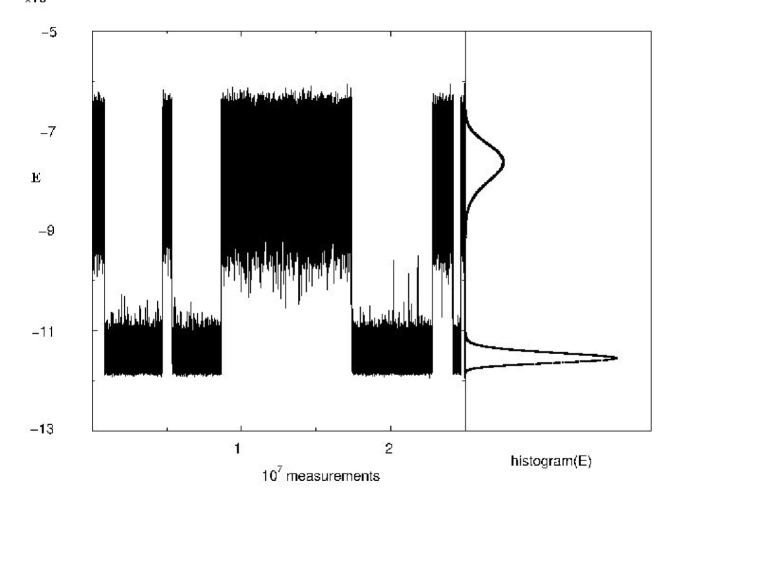
Figure 1: Energy time series and corresponding energy histogram for $L=20$ and $\beta_{MC}=0.5064$

In Fig. 1 we present the energy time-series for the $L=20$ and $\beta_{MC}=0.5064$ simulation run. The expected characteristic behaviour of a first order phase transition can be clearly seen. The system remains in one of the two coexisting phases for a long period of time. The energy histogram for the full series is also presented in the Figure. The similar height of the two peaks confirms that the simulation was performed very near the pseudo-critical inverse temperature.

In addition to the qualitative analysis of the histograms, we have computed the specific heat, magnetic susceptibility and the energetic Binder parameter at nearby values of $\beta_{MC}$ by means of standard reweighting techniques [12]. These observables are defined as

$$C(\beta) = \frac{\beta^{2}}{V}(\langle E^{2}\rangle-\langle E\rangle^{2}),$$ (6)

$$\chi(\beta) = \frac{\beta^{2}}{V}(\langle M^{2}\rangle-\langle M\rangle^{2}),$$ (7)

$$B(\beta) = 1-\frac{\langle E^{4}\rangle}{3\langle E^{2}\rangle^{2}}.$$ (8)

In Table 3 we show the extrema of the magnitudes defined above, together with their pseudo-critical inverse temperatures. The error bars of these quantities have been estimated splitting the time-series data into 50 bins, which were then jackknived to decrease the bias in the analysis of reweighted data.

5 Analysis of results

Once we have the results from the numerical simulation on finite lattices, we can proceed to analyze the data by fitting to the scaling laws of Table 1.

In Table 4 we show the results of fitting the pseudo-critical $\beta$s of $C_{\rm max}$, $\chi_{\rm max}$ and $B_{\rm min}$ to the ansatz

$$\beta_{\rm max}(L)=\beta_{c}+\frac{a_{1}}{L}+\frac{a_{2}}{L^{2}}$$ (9)

suggested by the finite-size scaling laws presented in Table 1. For $\chi_{\rm max}$ and $B_{\rm min}$ the fits were rather poor if $L=10$ was included, so it was discarded. For $C_{\rm max}$ both sets $L=10-20$ and $L=12-20$ were fitted. Focusing on the $L=12-20$ fits, we can discern only very minor differences in the estimated $\beta_{c}$ depending on the observable used to extract it. These are so small that we can safely average to obtain

$$\beta_{c}=0.54757\pm 0.00063$$ (10)

Since the $\beta_{c}$’s extracted from the three observables were not independent, we have kept the error bar common to them all. In Fig. 2 we depict the fit for $\beta^{C}_{\rm max}(L)$ in the range $L=10-20$. The error bars in the Figure are so small that they show up only as horizontal dashes.

The results of the fits to the specific heat and susceptibility maxima, $C_{\rm max}$ and $\chi_{\rm max}$, together with the energetic Binder parameter minimum are summarized in Table 5. The goodness-of-fit, $Q$, is excellent for the three observables.

Note that the surface correction coefficients $a_{1}$ and $b_{1}$ are, in absolute value, from one to two orders of magnitude larger than the coefficients $a_{2}$ and $b_{2}$ of the dominant contribution $V=L^{3}$. It is precisely this fact which makes it necessary to use the scaling ansatz $C_{\rm max}(L)=a_{0}+a_{1}\,L^{2}+a_{2}\,L^{3}$, and allows us to estimate the corrections to the leading term.

6 Conclusions

We have performed a numerical simulation of the 3d Gonihedric Ising model at $\kappa=0$ in order to determine the thermodynamic characteristics of its phase transition. Previous analysis suggested the existence of a first order phase transition, but a complete finite size analysis of the transition was not carried out. The special features of this model, which requires a simulation where three perpendicular spin planes need to be fixed during the simulation, do not allow a direct application of the standard finite size scaling laws for periodic boundary conditions at a first order transition. In fact, to keep these planes fixed is equivalent to performing a simulation with fixed boundary conditions (F.B.C.), giving rise to the need for a different set of scaling laws. They were reviewed in Sec. 3. Our numerical analysis of the thermodynamic quantities has shown that the critical behavior of the 3d Gonihedric Ising model is perfectly described in terms of F.B.C. scaling laws. As a result of this work, we have been able to accurately determine the inverse critical temperature of the model, i.e. $\beta_{c}=0.54757(63)$. Furthermore, our simulation has extended the verification of the F.B.C. scaling laws to a three dimensional lattice model.

Acknowledgements

M.B. and R.V. acknowledge financial support from MCyT project BFM 2002-02588 and CIRIT project SGR-00185, D.J. acknowledges the partial support of EC network grant HPRN-CT-1999-00161.

Table 1: Scaling laws for Periodic versus Fixed Boundary Conditions.

	P.B.C.	F.B.C.
$\beta_{c}^{peaks}(L)=$	$\beta_{c}(\infty)+\frac{\theta_{1}}{L^{d}}+O(\frac{1}{L^{2d}})$	$\beta_{c}(\infty)+\frac{a_{1}}{L}+O(\frac{1}{L^{2}})$
$C_{max}(L)=$	$\gamma_{0}+\gamma_{2}L^{d}+O(\frac{1}{L^{d}})$	$c_{0}+c_{2}L^{d}+O(L^{d-1})$
$\chi_{max}(L)=$	$\delta_{0}+\delta_{2}L^{d}+O(\frac{1}{L^{d}})$	$e_{0}+e_{2}L^{d}+O(L^{d-1})$
$B_{min}(L)=$	$\Phi_{0}+\frac{\Phi_{1}}{L^{d}}+O(\frac{1}{L^{2d}})$	$B_{0}+\frac{B_{1}}{L}+O(\frac{1}{L^{2}})$

Table 2: Monte Carlo parameters of the simulation. $L^{3}$ is the lattice size, $n_{\rm therm}$ the number of Monte Carlo sweeps during thermalization (in thousands), and $n_{\rm prod}$ the number of production runs (in millions). Measurements were taken every $n_{\rm flip}=4$ Monte Carlo sweeps for all the simulations, except the latest; the number of bins was 50.

$L$	$\beta_{MC}$	$n_{\rm therm}$	$n_{\rm prod}$	$n_{\rm flip}$	$\tau_{\bf\rm e}$	$\frac{n_{\rm therm}/n_{\rm flip}}{\tau_{\bf\rm e}}$	$\frac{n_{\rm prod}/n_{\rm flip}}{2\,\tau_{\bf\rm e}}$
10	0.4580	500	20	4	25	5 000	100 000
12	0.4748	500	20	4	45	2 778	55 556
14	0.4864	500	20	4	278	450	8 993
15	0.4910	500	20	4	1 011	124	2 473
18	0.5013	2 500	22	4	24 871	25	111
20	0.5064	36 500	200	8	216 098	21	58

Table 3: Extrema for the (finite lattice) specific heat, $C_{\rm max}$, the susceptibility, $\chi_{\rm max}$, and the energetic Binder parameter, $B_{\rm min}$, together with their respective pseudo-critical inverse temperatures.

$L$	$\beta_{\rm max}^{C}$	$C_{\rm max}$	$\beta_{\rm max}^{\chi}$	$\chi_{\rm max}$	$\beta_{\rm min}^{B}$	$B_{\rm min}$
10	0.457919(21)	5.6945(79)	0.456842(22)	7.042(12)	0.455064(21)	0.638537(47)
12	0.474753(16)	12.120(21)	0.474470(15)	16.305(31)	0.473468(16)	0.635656(61)
14	0.486349(21)	25.172(45)	0.486275(21)	36.264(73)	0.485647(21)	0.628430(85)
15	0.490922(30)	34.900(76)	0.490884(30)	51.91(13)	0.490374(30)	0.62432(12)
18	0.501280(72)	78.99(38)	0.501273(72)	128.10(69)	0.500979(72)	0.61246(36)
20	0.506366(69)	121.57(52)	0.506364(69)	206.61(99)	0.506149(69)	0.60620(36)

Table 4: Pseudo-critical inverse temperature fits. Q is the goodness-of-fit.

range L’s	$\beta^{C}_{\rm max}(L)=\beta_{c}+a_{1}/L+a_{2}/L^{2}$				$\beta^{\chi}_{\rm max}(L)=\beta_{c}+d_{1}/L+d_{2}/L^{2}$				$\beta^{B}_{\rm max}(L)=\beta_{c}+e_{1}/L+e_{2}/L^{2}$
	Q	$\beta_{c}$	$a_{1}$	$a_{2}$	Q	$\beta_{c}$	$a_{1}$	$a_{2}$	Q	$\beta_{c}$	$a_{1}$	$a_{2}$
10 – 20	0.89	0.54868(34)	-0.7848(84)	-1.229(51)
12 – 20	0.73	0.54867(63)	-0.785(18)	-1.23(12)	0.85	0.54730(63)	-0.736(18)	-1.65(12)	0.86	0.54674(63)	-0.711(18)	-2.02(12)

Table 5: Fits on the extrema of $C_{\rm max}$, $\chi_{\rm max}$ and $B_{\rm min}$.

range L’s	$C_{\rm max}(L)=a_{0}+a_{1}\,L^{2}+a_{2}\,L^{3}$				$\chi_{\rm max}(L)=b_{0}+b_{1}\,L^{2}+b_{2}\,L^{3}$				$B_{\rm min}(L)=B_{0}+B_{1}/L+B_{2}/L^{2}$
	Q	$a_{0}$	$a_{1}$	$a_{2}$	Q	$b_{0}$	$b_{1}$	$b_{2}$	Q	$B_{0}$	$B_{1}$	$B_{2}$
10 – 20	0.16	14.43(17)	-0.4434(36)	0.03561(20)					0.014	0.4992(15)	2.851(35)	-14.57(21)
12 – 20	0.098	14.79(52)	-0.4491(83)	0.03587(40)	0.62	39.92(92)	-1.035(15)	0.07257(73)	0.21	0.5065(30)	2.643(84)	-13.12(57)

Figure 2: Finite-size scaling analysis of the pseudo-critical $\beta^{C}_{\rm max}$ in the range $L=10-20$ by means of the ansatz $\beta^{C}_{\rm max}(L)=\beta_{c}+a_{1}/L+a_{2}/L^{2}$. The infinite volume critical point obtained from the fit is $\beta_{c}=0.54868(34)$, with a goodness-of-fit $Q=0.89$.

References

- [1] M. Baig and R. Villanova. Phys. Rev. B 65, 094428 (2002).
- [2] C. Borgs and R. Kotecký, Journ. Stat. Phys. 61, 79 (1990); ibidem 79, 43 (1995). I. Medved, diploma Thesis. Charles University. Prague.
- [3] M. Baig, D. Espriu, D.A. Johnston and R.P.K.C. Malmini, J. Phys. A 30, 405 (1997); ibidem 30, 7695 (1997).
- [4] A. Cappi, P. Colangelo, G. Gonnella, and A. Maritan, Nucl. Phys. B370, 659 (1992). W. Selke Phys. Rep. 170, 213 (1988).
- [5] R.V. Ambartsumian, G.S. Sukiasian, G.K. Savvidi, and K.G. Savvidy, Phys. Lett. B275, 99 (1992). G.K. Savvidy and K.G. Savvidy, Mod. Phys. Lett. A8, 2963 (1993). G.K. Savvidy and K.G. Savvidy, Int. J. Mod. Phys. A8, 3993 (1993).
- [6] G.K. Savvidy and F.J. Wegner, Nucl. Phys. B413, 605 (1994). G.K. Savvidy and K.G. Savvidy, Phys. Lett. B324, 72 (1994); ibidem B337, 333 (1994). G.K. Savvidy, K.G. Savvidy, and P.G. Savvidy, Phys.Lett. A221, 233 (1996). G.K. Savvidy, K.G. Savvidy and F.J. Wegner,Nucl. Phys. B443, 565 (1995).
- [7] G.K. Bathas, E. Floratos, G.K. Savvidy, and K.G. Savvidy, Mod. Phys. Lett. A 10, 2695 (1995). R. Pietig and F.J. Wegner, Nucl. Phys. B466, 513 (1996).
- [8] T. Sterling and J. Greensite, Phys. Lett. B121, 345 (1983). M. Karowski and H.J. Thun, Phys. Rev. Lett. 54, 2556 (1985). M. Karowski J. Phys. A19 (1986) 3375.
- [9] D.A. Johnston and R.P.K.C. Malmini, Phys. Lett. B378, 87 (1996).
- [10] A.D. Sokal in Monte Carlo Methods in Statistical Mechanics: Foundations and New Algorithms, lecture notes, Cours de Troisième Cycle de la Physique en Suisse Romande, Lausanne (1989). N. Madras and A.D. Sokal, J. Stat. Phys. 50, 109 (1988). W. Janke, Monte Carlo Simulations of Spin Systems, in: Computational Physics: Selected Methods – Simple Exercises –Serious Applications, eds. K.H. Hoffmann and M. Schreiber (Springer, Berlin, 1996), p. 10.
- [11] R.G. Miller, Biometrika 61, 1 (1974). B. Efron, The Jackknife, the Bootstrap and other Resampling Plans (SIAM, Philadelphia, PA, 1982).
- [12] A.M. Ferrenberg and R.H. Swendsen, Phys. Rev. Lett. 61, 2635 (1988).