Parametric Amplification of Nonlinear Response of Single Crystal Niobium

Abstract

Giant enhancement of the nonlinear response of a single crystal Nb sample, placed in a pumping ac magnetic field, has been observed experimentally. The experimentally observed amplitude of the output signal is about three orders of magnitude higher than that seen without parametric pumping. The theoretical analysis based on the extended double well potential model provides a qualitative explanation of the experimental results as well as new predictions of two bifurcations for specific values of the pumping signal.

I Introduction

It was well established in the sixties that nucleation of the superconductivity in magnetic field parallel to the sample surface begins when magnetic field $H$ becomes lower than surface nucleation field $H_{c3}$ ($H_{c3}\approx 1.69H_{c2}$) DG . The experiments at low frequencies reveal a nonlinear nature of the ac response of the superconductors in surface superconducting state ROLL ; JOIN . A critical state model for the superconducting surface sheath was used for theoretical explanation of the experimental findings ROLL ; FINK . Recently our study of the nonlinear properties of single crystal Nb showed that the critical state model hardly fits the new experimental data and a simplified two level model was used for the theoretical explanation of the experiment MT .

The above mentioned experiments in superconducting materials related to the nonlinear effects such as harmonic generation or rectification. But there is another class of nonlinear effects - parametric phenomena. Parametric phenomena are important in fundamental physics and for applications. Parametric amplification of the weak microwave signals in Josephson junctions were studied in detail in thew seventies (see BP and references therein). Experimental observations of parametric amplification of the weak microwave signals were possible because of the nonlinearity of the Josephson junction BP . To the best of our knowledge parametric phenomena in surface superconducting states of bulk superconductors has yet to be studied.

The present study is a continuation of our previous experimental work and the theoretical analysis of the nonlinear dynamics in the surface superconducting states of a single crystal Nb MT . In these experiments the dc and low-amplitude high-frequency ac fields have been applied along the long axis of a sample. It was found that in the steady-state regime the nonlinear effects exist only in the surface superconducting phase. A unique aspect of this system is that the non-linearity does not exist a priory, but rather appears only in the presence of an imposed dc field.

The new experiments have been performed in the same system, subjected to an additional low-frequency excitation field, and the amplitude of the output signal was measured as a function of the amplitudes of the external fields including that of the ac excitation field. In this experiment the nonlinearity of the system plays a double role. Usual parametric experiments deal with two signals. The system is excited by weak and strong (pumping) signals. The frequency of the pumping signal is twice as large as the frequency of the weak signal. Due to the nonlinearity of the system, power from the pumping signal transfers to the weak signal BP . In our experiment, the system was excited by an amplitude modulated ac field having some carrier and modulation frequencies. The spectrum of the ac field does not contain the modulation frequency. The modulation frequency in a system appears when the sample is in a nonlinear state. Only for a nonlinear system a pumping signal at a frequency twice as large as the modulation frequency affects the nonlinear response. The theoretical analysis, based on the extended double well potential model of two surface states, provides a qualitative explanation of the experimental data and predicts some new results which are partially confirmed by experiment.

II Sample preparation and experimental technique

A rectangular ($10\times 3\times 1$ mm³) sample was cut by an electric spark from a single crystal niobium bar which had been fabricated by electron beam melting of high purity Nb precursor. The [100] crystalline direction is parallel to the long axis of the sample and the [010] direction is perpendicular to the sample plane. After mechanical and chemical polishing the crystal was annealed for one hour at T=1800 K under a vacuum of 10^-7 Torr. These procedures provided a high quality sample, as confirmed by the high resistance ratio $R_{300K}/R_{10K}\approx 300$ and unperturbed critical temperature $T_{c}=9.15$ K. The details of the employed Nb crystal characterization, including H-T phase diagram, have been published elsewhere MT .

The nonlinear response experiment was carried in a modified commercial SQUID magnetometer, also used for measurements of the dc magnetic properties. The Nb rod was placed in dc and ac magnetic fields applied along the [100] direction. The excitation ac field generated by a high frequency generator operating in a constant current regime had the form of an amplitude modulated ac field $h(t)=h_{0}(1+\alpha\cos\Omega t)\cos\omega t$. Typical values of above parameters were $0<h_{0}<0.4$ Oe, $\alpha\approx 0.9$, $\omega/2\pi=3.2$ MHz, and $\Omega/2\pi=1455$ Hz. A parametric pumping field $h_{p}(t)=h_{2\Omega}\cos(2\Omega t)$ was achieved using a copper solenoid of the commercial SQUID magnetometer system.

A block diagram of the experimental setup is shown in Fig. 1. A 65-turn primary copper coil driven by a high frequency generator (HP3325A) produces an amplitude modulated ac field $h(t)$. Signals with frequencies $\Omega$ and $2\Omega$ were generated by an Agilent 33250A model generator. The 1500 turn secondary copper coil was wound directly on the primary coil. The length of both coils was 15 mm. The voltage drop over the secondary coil was measured by a lock-in amplifier (EG&G 7265). The modulation frequency $\Omega$ was used as a reference frequency for the lock-in amplifier. The ac field amplitudes $h_{0}$ and $h_{2\Omega}$ were measured by an additional small probe coil wound under the primary coil. For the sake of clarity a probe coil is not shown in Fig. 1.

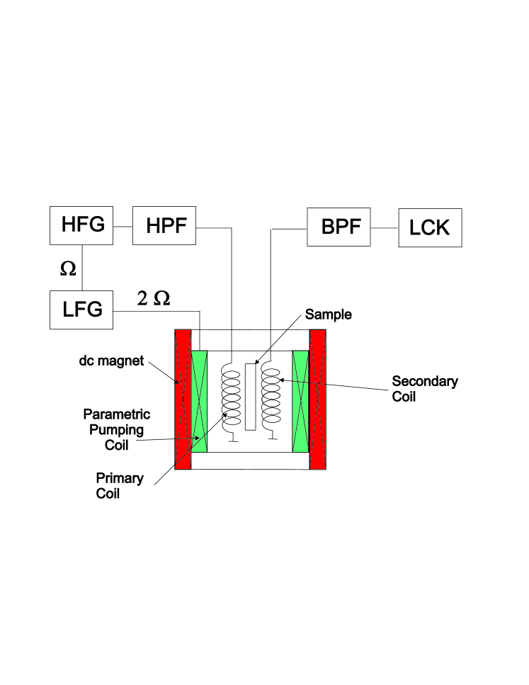
Figure 1: (Color online) Block diagram of the experimental setup. HFC - high frequency generator, LFG - low frequency generator, HPF and BPF - high and band pass filters, LCK - lock-in amplifier.

One should note that the ratio between the pumping frequency and the modulation frequency was equal exactly to 2 in our experimental setup.

When the ac excitation is applied to a superconducting sample in the nonlinear state, the magnetic moment of the sample oscillates at the harmonics of the fundamental frequency $\omega$, at frequencies $\omega\pm\Omega$, and at the frequency of modulation $\Omega$ and its harmonics. The secondary coil converts these magnetic moment oscillations into an ac voltage signal. In the experiments we have measured, by means of lock-in detection, the amplitude $A_{\Omega}$ of the signal at frequency $\Omega$ as a function temperature, dc magnetic field $H$, ac field amplitude $h_{0}$ and amplitude of parametric pumping $h_{2\Omega}$.

III Experimental results.

Here we restrict our consideration to the experimental data which allow a direct theoretical explanation. Fig. 2 shows the field dependence of the rectified signal $A_{\Omega}$ measured at $T=7.5$ K for different amplitudes of $h_{2\Omega}$ compared with the data obtained in the absence of a pumping field, $h_{2\Omega}=0$.

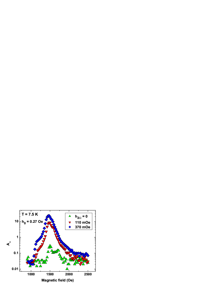
Figure 2: (Color online) The amplitude of the output signal$A_{\Omega}(H)$ as a function of the dc field $H$ at different pumping amplitudes $h_{2\Omega}$.

As evident from Fig. 2 the application of parametric pumping leads to a giant enhancement of the rectified signal. Under our experimental conditions the enhancement of $A_{\Omega}$ reaches two hundred times, the signal in absence of parametric pumping. The present result confirms our resent observation MT that under stationary conditions the pronounced rectified signal appears only in the surface superconducting state.

The measurements of $A_{\Omega}$ as a function of $h_{2\Omega}$ for constant $H$ and $h_{0}$ provides interesting information about nonlinearity of the sample. In figures 3 and 4 we present the amplitude of the output signal $A_{\Omega}$ as a function of the amplitude of the pumping field $h_{2\Omega}$ for different magnitudes of $H$ and amplitudes $h_{0}$ of the dc and ac fields. Fig. 3 shows that increasing the amplitude of excitation, $h_{0}$, does not always lead to a straight enhancement of the amplitude of the nonlinear response. Nonlinear systems with strong nonlinearity frequently demonstrate this type of behavior.

The experimental data presented in Figs. 3, 4 are very complicated. In order to straighten out this many-parameter dependence a theoretical basis is needed which we will discuss in the next section.

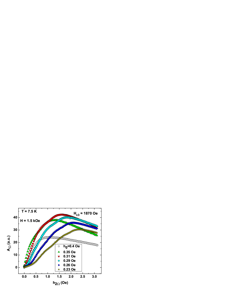
Figure 3: (Color online) The amplitude of output signal $A_{\Omega}$ as a function of pumping amplitude $h_{2\Omega}$.

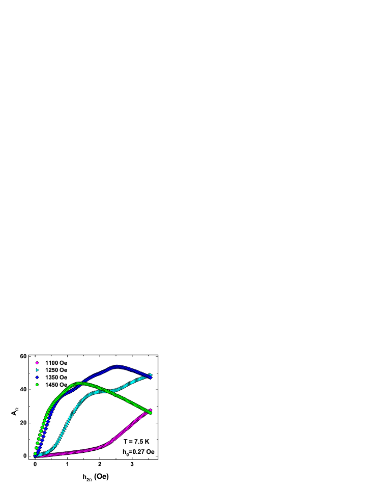
Figure 4: (Color online) The amplitude of output signal $A_{\Omega}$ as a function of pumping amplitude $h_{2\Omega}$ at different magnitude of magnetic field $H$.

IV Theoretical analysis and discussions

In the experiments described above the magnetic field $H$ is the large constant field, and $h\left(t\right)$ is a low amplitude ac field. It turns out that for a given value of $H$ there are many superconducting states which can be labelled by the number $n$ of fluxons pinned in this level, and each of them corresponds to a local minima in the free energy. For the theoretical description of the nonlinear response we use the well-known Landau-Khalatnikov equation of motion for the magnetic moment $M$ of the surface state

$$\frac{dM}{dt}=-\Gamma\frac{\partial G}{\partial M}$$ (1)

where $\Gamma$ is a phenomenological coefficient which hereafter is assumed to be equal to unity, ($\Gamma=1$), and the total Ginzburg-Landau free energy $G$  is composed of a series of parabolic branches, $G=\sum G_{n}$, corresponding to the number $n$ of the single flux quantum $\Phi_{0}$ in the state $G_{n}$ ROLL ,

$$G_{n}=\frac{\pi R^{2}}{8}\left(M-M_{n}\right)^{2}-\epsilon\left(1-\frac{2M}{H_{c_{3}}}\right)$$ (2)

where $M_{n\text{ }}=n\Phi_{0}/\pi R^{2},$ and $\epsilon$ is the energy to nucleate a fluxon.

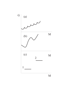
Figure 5: (a) Schematic representation of the free energy of a system as a function of the magnetic moment ; (b) a tilted double well system ; (c) a two-level system.

According to Eq. (2), the free energy as a function of an external field is composed of a series of parabolic branches (corresponding to different $n$) with centers located on an ascending curve (Fig. 5).

Instead of considering the free energy Eq. (2) we restrict ourselves to the relevant initial and final states. In line with this assumption let us replace the many-wells system shown in Fig. 5a, by a tilted double-well system (Fig. 5b), where the right minimum at $M=0$ corresponds to the surface superconducting nucleation field $H_{C_{3}}$, and the left minimum is related to some magnetic moment $M$ induced by an external field $H.$ The distance between the minima is proportional to $H_{C_{3}}-H,$

Hence, the adopted form of the free energy

$$\frac{4G}{\pi R^{2}}=-\frac{M^{2}}{2}+\frac{p^{2}M^{4}}{4}+\gamma M$$ (3)

contains two parameters

$$p\approx\left(H_{C_{3}}-H\right)^{-1}\text{ \ : \ }\gamma=\frac{2\epsilon}{H_{c_{3}}}$$ (4)

Note that in our previous work MT we have used a model with two discrete levels (Fig. 5c). For discrete levels the continuous dynamics, Eq. (1), is replaced by jumps between the potential minima, and the appropriate rate equation in the presence of the external ac field,  $h\left(t\right)$, can be solved by using the adiabatic approximation. In such a manner we have accounted for the main experimental results such as a set of maxima of the output signal as a function of $H$ for different fixed ac strength $h_{0}$ MT .

In the experiments analyzed in the previous publication MT the external ac field was the sum of three monochromatic waves

$$\begin{array}[]{c}h(t)=h_{0}\cos(\omega t)+0.45h_{0}[\cos(\omega+\Omega)t\\ +\cos(\omega-\Omega)t]\end{array}$$ (5)

one with a frequency $\omega$, and two with satellite frequencies $\omega\pm\Omega$, where $\Omega\ll\omega$. This multifrequency excitation of a non-linear system allows one to detect a signal at low frequency $\Omega$.

Unlike the previous work, in the new experiments described in the previous sections , an additional pumping field $h_{p}(t)=h_{2\Omega}cos(2\Omega t)$ was applied to the system. Substituting this field together with Eqs. (2-4) into Eq. (1) one gets

$$\begin{array}[]{c}\frac{4}{\pi R^{2}\Gamma}\frac{dM}{dt}=M-(\frac{1}{H_{c3}-H})^{2}M^{3}+2\frac{\epsilon}{H_{c3}}\\ +h_{0}\cos\omega t+0.45h_{0}[\cos(\omega+\Omega)t\\ +\cos(\omega-\Omega)t]+h_{2\Omega}\cos 2\Omega t\end{array}$$ (6)

Since $\Omega\ll\omega$, one can decompose $M\left(t\right)$ into a sum of two terms as follows GIT

$$\begin{array}[]{c}M\left(t\right)=x\left(t\right)+\frac{h_{0}}{\omega}\sin\left(\omega t\right)+\\ \frac{0.45h_{0}}{\left(\omega+\Omega\right)}\sin\left[\left(\omega+\Omega\right)t\right]+\\ \frac{0.45h_{0}}{2\left(\omega-\Omega\right)}\sin\left[\left(\omega-\Omega\right)t\right]\end{array}$$ (7)

The first term on the right-hand side of Eq. (7) will be assumed to vary significantly only over times of the order of $t$, while the other terms vary rapidly. Substituting (7) into (6) one can perform an averaging over a single cycle time of $\sin\left(\omega t\right)$. All odd powers of $\sin\left(\omega t\right)$ vanish under the average while the $\sin^{2}\left(\omega t\right)$ term will give $\frac{1}{2}.$ Finally, one obtains the following equation for $A\left(t\right),$ the mean value of $M\left(t\right)$ during the oscillation period, $A\left(t\right)=$ $<M\left(t\right)>,$

$$\begin{array}[]{c}\frac{dA}{d\tau}-A\left[a-b\cos\left(\Omega t\right)-c\cos\left(2\Omega t\right)\right]\\ +p^{2}A^{3}+\beta=\frac{h_{2\Omega}}{h_{0}}\cos\left(2\Omega t\right)\end{array}$$ (8)

where we have introduced the dimensionless parameters

$$\begin{array}[]{c}A=\frac{M}{h_{0}}\text{;\ }\tau=\frac{4t}{\pi R^{2}}\text{;\ }p^{2}=\left(\frac{h_{0}}{H_{c3}-H}\right)^{2}\text{; }\\ \beta=\frac{\gamma}{h_{0}}\text{\ }a=1-\frac{9.9p^{2}}{4\left(\omega\pi R^{2}\right)^{2}}\text{; }\\ b=\frac{3.3p^{2}}{\left(\omega\pi R^{2}\Gamma\right)^{2}}\text{ ; \ }c=\frac{3.3p^{2}}{4\left(\omega\pi R^{2}\right)^{2}}\end{array}$$ (9)

It is clear now that for dimensionless amplitudes of the output and the input signal, $\frac{M}{h_{0}}$ and $\frac{h_{2\Omega}}{h_{0}}$, the main parameter which defines the input-output relations is $\left(\frac{h_{0}}{H_{c3}-H}\right)$ while the phenomenological parameter $\beta$ is less important.

Based on the theory described above we may now redraw the experimental data shown in Figs. 3 and 4. In order to straighten out these experimental data one has to use the scaled dimensionless coordinates $\frac{A}{h_{0}}$ and $\frac{h_{2\Omega}}{h_{0}},$ and grouping together the experimental points  corresponding to the same value of the parameter $\frac{h_{0}}{H_{c3}-H}.$ These regrouping data from Figs. 3 and 4 are show in Fig. 6.

Figure 6: (Color online) Experimental data redrawn in the dimensionless amplitudes of the output and the input signals, $\frac{A_{\Omega}}{h_{0}}$ and $\frac{h_{2\Omega}}{h_{0}}$ for the constant value of the dimensionless parameter $\frac{h_{0}}{H_{c3}-H}$.

As one can see from this figure the experimental data are now well ordered as they should be according to Eq. (8). The small differences between different curves might be attributable to the different values of parameter $\beta$. The regrouping procedure was used for the evaluation of $H_{c3}$ from the experimental data as well. The universal behavior $A_{\Omega}(h_{2\Omega})$ occurs possible for different temperatures. Fig. 7 demonstrates this type of universal behavior for $A_{\Omega}(h_{2\Omega})$ in dimensionless coordinates at $T=7.5$ K and $T=6$ K .

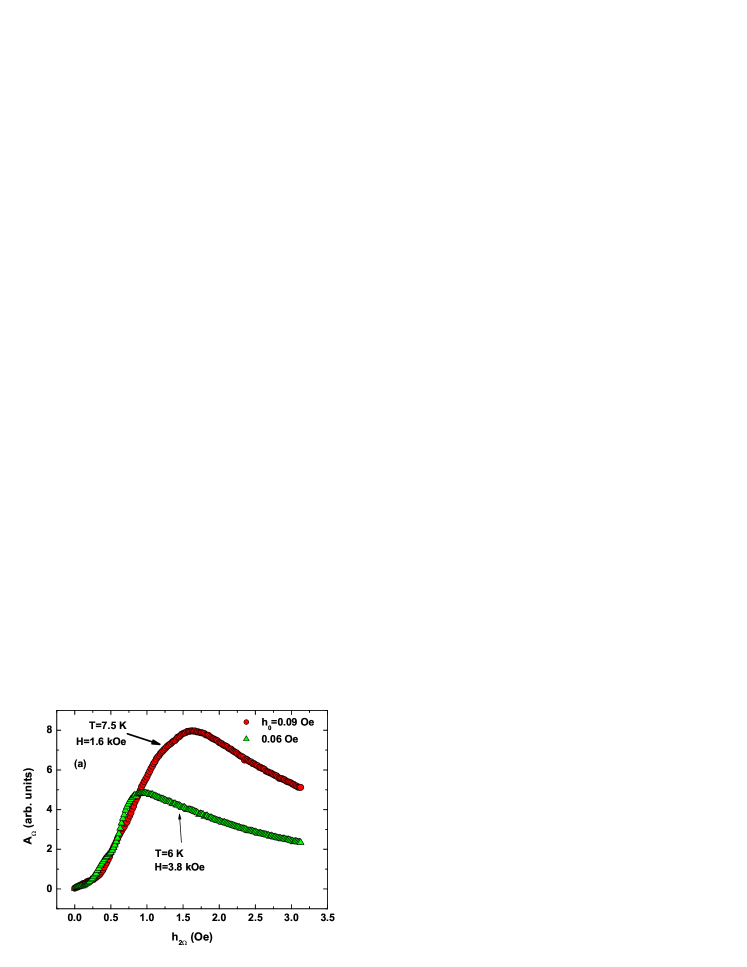
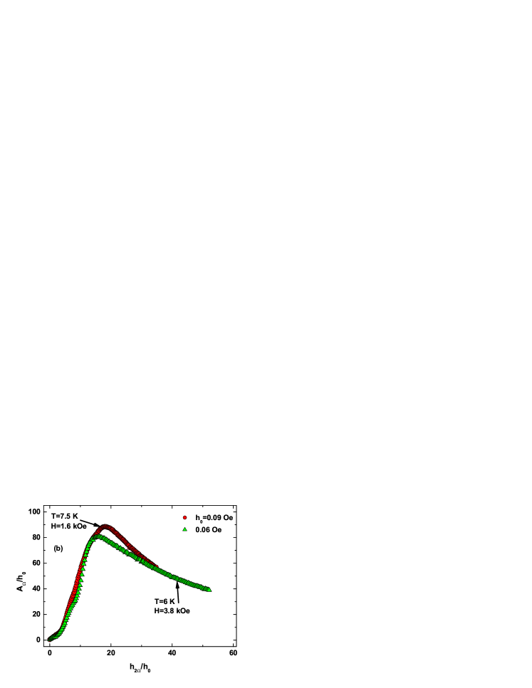
Figure 7: (Color online) (a) $A_{\Omega}(h_{2\Omega}$ dependencies for $T=7.5$ K and $T=6$ K for the constant value of the dimensionless parameter $\frac{h_{0}}{H_{c3}-H}$. (b) The same experimental data redrawn in the dimensionless amplitudes of the output signal and the parametric pumping amplitude, $\frac{A_{\Omega}}{h_{0}}$ and $\frac{h_{2\Omega}}{h_{0}}$

The universal form of the curves in Figs. 6,7 suggests the validity of our theory. Eq. (8) describes the overdamped Duffing oscillator with parametric and forced periodic excitations. Although an extensive literature is devoted to an investigation of the Duffing oscillator(NA ), the periodic excitations were analyzed only for the underdamped case (FX ). We have performed comprehensive numerical integrations of Eq. (8). A typical result of these calculations for some values of the parameter $\frac{h_{0}}{H_{c3}-H}$ is shown in Fig. 8.

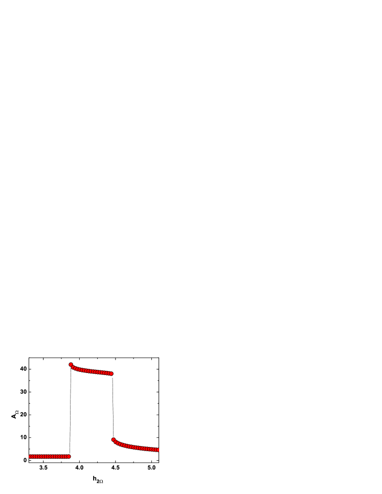
Figure 8: (Color online) Two bifurcations of the amplitude of the output signal $A_{\Omega}$ as a function of the amplitude $h_{2\Omega}$ of the pumping signal.

Several conclusions can be reached from the analysis of this and similar graphs :

1. Over a wide range of the parameter $\frac{h_{0}}{H_{c3}-H},$ there are two bifurcations at small (”left”) and large (”right” ) values of the amplitudes of the pumping field.

2. With a decrease of $(\frac{h_{0}}{H_{c3}-H})^{2}$, the coefficient which multiplies the nonlinear term, the right bifurcation occurs at a larger amplitude of the pumping signal ,and the jump becomes larger.

3. With a decrease of $b$ (and $c$) which describe the parametric excitation, the left bifurcation occurs at a somewhat larger pumping amplitude, and the jump becomes slightly larger.

The currently available experimental data show at least qualitative agreement with the suggested theory:

a) Comparison of the experimental graphs in figures 3
and 4, and their scaling treatment shown in Figs. 6,7 clearly proves that the theoretical model addresses the main features of the experimental data.

b) The giant increase of the output signal in the presence of the pumping field shown in Fig. 2, is present in our theoretical model as well. For instance, for $p=2\ast 10^{-2}$  , equation (8) shows a two order of magnitude increase in $A_{\Omega}$ in going from $h_{2\Omega}=0$ to $h_{2\Omega}=50.$

c) The presence of the left bifurcation can be seen from experimental graph 9 which shows $A_{\Omega}$ as a function of  h_2Ω for different values of $H$.

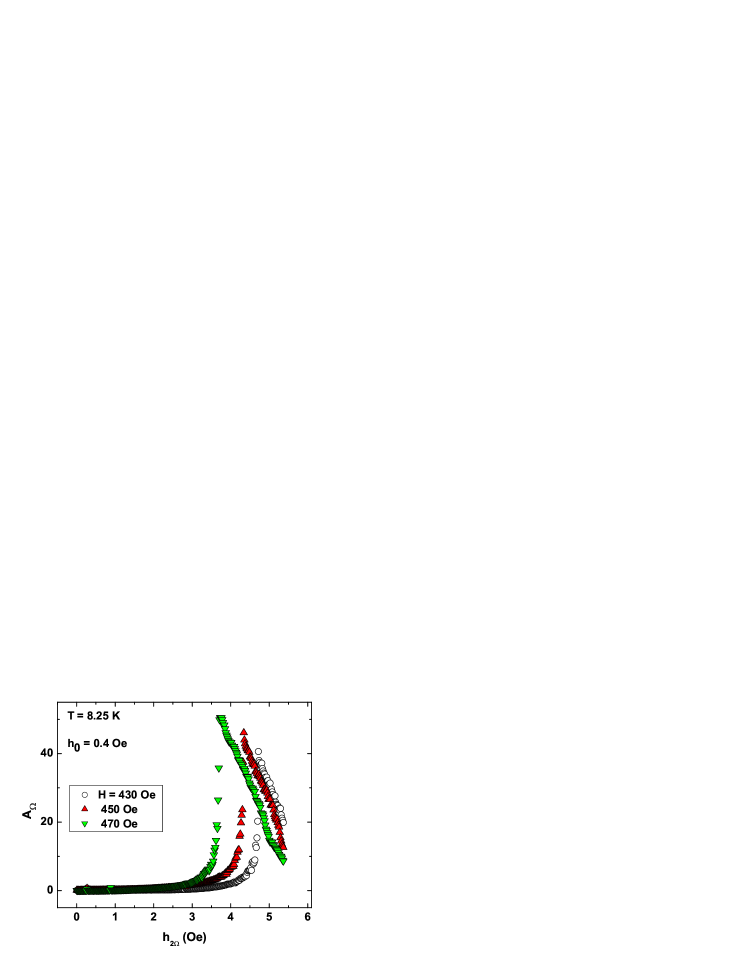
Figure 9: (Color online) Experimental data describing the dependence of the amplitude of the output signal $A_{\Omega}$ as a function of the amplitude of the pumping signal $h_{2\Omega}$ for different values of $H$.

The values of $h_{2\Omega}$ at maxima are shown in Fig. 10 for different $H$. In the same figure we show also the same quantities obtained from Eq. (8). Since in the theoretical analysis we omit some constant coefficients ($\Gamma=1,p\approx\left(H_{C_{3}}-H\right)^{-1}$, etc.), in the comparison of theoretical results with experimental data one has to set one of the points on the theoretical curve with one on the experimental curve, which has been done in Fig. 10.

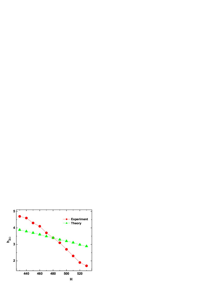
Figure 10: $h_{2\Omega}$ of maxima obtained from experimental graphs Fig. 9 and from the theoretical analysis of Eq. 8.

Both curves are almost straight lines with the correct sign of the slope, i.e., we conclude that our theoretical model gives at least semi-quantitative agreement with experiment. However, one cannot see the right bifurcation on the experimental graph 8 which is, probably, connected with some ignored factor in our theory which smears this bifurcation. Another possible explanation lies in the fact that in order to see in the experiment the right bifuracation, one needs the higher amplitudes of the pumping signal which cannot be achieved with the existing experimental set up.

V Summary

We have performed an extensive experimental study of the non-linear response in surface superconducting states of single crystal niobium. Application of a pumping ac magnetic field results in a giant (about three order of magnitude) increase of the amplitude of the output signal. The theoretical analysis, based on the extend double well potential model, provides a qualitative explanation of the experimental results as well as predicting a new phenomenon, the abrupt change (bifurcation) of the nonlinear response in ac driven superconductors. The latter effect, in its turn was partially supported by experiment.

VI Acknowledgments

The work at the Hebrew University was supported by the Klatchky foundation. The authors are deeply grateful to Dr. S.I. Bozhko and Dr. A.M. Ionov (ISSP RAS, Chernogolovka, Moscow district, Russia) for the sample preparation. We thank Professors I. Felner, B.Ya. Shapiro, Dr. V. Genkin and Dr. G. Leviev for useful discussions. M.I.T. wishes to thank G. Greenwald for the providing nonstandard electronic devices.

References

- (1) P.G. de Gennes, Superconductivity of Metals and Alloys (W.A.Benjamin, New-York, 1966).
- (2) R. W. Rollins and J. Silcox, Phys. Rev. 155, 404 - 418 (1967).
- (3) W.C.H. Joiner and M.C. Ohmer, Sol. St. Comm., 8, 1811 (1970).
- (4) H.J. Fink, Phys. Rev. Lett. 16, 447 (1966).
- (5) M.I. Tsindlekht, I. Felner, M. Gitterman, B.Ya. Shapiro, Phys. Rev. B 62, 4073 (2000).
- (6) A. Barone, G. Paterno, Physics and Applications of the Josephson Effect (J. Wiley & Sons, New York, 1982).
- (7) M. Gitterman, J. Phys. A 34, L355 (2001).
- (8) A.H. Nayefeh, Perturbation methods (Wiley, New York, 1973).
- (9) Fagen Xie, Gang Hu, Phys. Rev. E51, 2773 (1995).