Off-equilibrium fluctuation-dissipation relation in a spin glass

Abstract

We report new experimental results obtained on the insulating spin glass $\mathrm{CdCr_{1.7}In_{0.3}S_{4}}$. Our experimental setup allows a quantitative comparison between the thermo-remanent magnetisation and the autocorrelation of spontaneous fluctuations of magnetisation, yielding a complete determination of the fluctuation-dissipation relation. The dynamics can be studied both in the quasi-equilibrium regime, where the fluctuation-dissipation theorem holds, and in the deeply ageing regime. The limit of separation of time-scales, as used in analytical calculations, can be approached by use of a scaling procedure.

1 Introduction

Despite their large diversity, glassy systems have many dynamical properties in common. In particular, a similar ageing behaviour can be observed in polymers, gelatins, or spin glasses Struik ; Mydosh . Stationarity cannot be reached in these systems in experimental, or even in geological times: they always remain out-of-equilibrium, even when not submitted to any external perturbation.

During a long period, the theoretical activity was concentrated on the study of the statics of glassy models. With the nineties, began the time of theoretical dynamical studies, first by numerical simulations, and then by analytical results on specific mean-field models Cugliandolo16 ; Cugliandolo01 ; Cugliandolo10 . From these studies, new concepts appeared, generalising the well known Fluctuation-Dissipation Theorem (FDT), which holds for equilibrated systems Callen00 ; Kubo .

In equilibrated systems with time translational invariance (TTI), FDT can be used to measure the temperature in an absolute way:

$$k_{B}T=\frac{\partial_{t_{w}}C(t-t_{w})}{R(t-t_{w})}$$ (1)

In this relation $C(t-t_{w})$ is the autocorrelation function of an observable (for instance the magnetisation $M(t)$) between two times, $t$ and $t_{w}$, and $R(t-t_{w})$ the response function associated with a pulse of the conjugate field at time $t_{w}$, $h(t)=\delta(t-t_{w})$. These quantities are two times quantities, but, as the system is TTI, they depend only on the time difference $t-t_{w}$ .

Spin glasses never reach equilibrium, and the time autocorrelation and the response function can not be reduced to one-time quantities. Therefore, the temperature cannot be defined on the basis of usual concepts. Nevertheless, it has been shown that, in specific models with low rate of entropy production, and using a generalisation of the FDT relation, a quantity that behaves like a temperature could be defined Cugliandolo10 , the “effective temperature”. The effective temperature for one given value of $C(t_{w},t)=C$ can be defined as:

$$k_{B}T_{eff}=\lim_{\begin{array}[]{c}{}_{t_{w}\rightarrow\infty}\\ {}_{C(t_{w},t)=C}\end{array}}\frac{\partial_{t_{w}}C(t_{w},t)}{R(t_{w},t)}$$ (2)

The only difference between relations 1 and 2 concerns the domains of validity. The generalised fluctuation-dissipation relation is valid for stationary systems (simply, $C$ and $R$ depend only on $t-t_{w}$ and $T_{eff}=T$), and it is also valid for every systems in the limit of small rate of entropy production. Glassy systems, in the limit of long waiting time are such systems. Some experiments have been set up to measure this effective temperature using frequency measurements in glassy systems Grigera00 ; Bellon00 ; Bellon03 .

To understand the meaning of the time limit in equation 2, it is helpful to refer to the so-called “Weak Ergodicity Breaking” (WEB) concept  JPBx1 . WEB was introduced first in the study of the dynamics of a random trap model very similar to the Random Energy Model (REM) Derridax0 . According to WEB scenario, two different contributions can be identified in the dynamics: a stationary one, corresponding to usual equilibrium dynamics in a metastable state (and then not relevant for ageing studies), and a second one, describing the long term evolution between many metastable states, which features the ageing properties.

This approach agrees well with an experimental fact: in glassy systems, the relaxation function can be decomposed in two distinct contributions Vincent00 :

• The first one is independent of the age of the system (it depends only on the observation time $t-t_{w}$), and governs the dynamics for the shorter observation times. Many results in spin glasses showed that the most appropriate form for the decay is a power law with a small exponent, $\alpha\approx 0.1$. This behaviour is consistent with the quasi-equilibrium noise power spectrum, which varies as $1/f^{1-\alpha}$. As this part is stationary, it should behave as in the equilibrated system: FDT should hold between the stationary part of the relaxation and the corresponding part of the autocorrelation, as shown in the section 4.1.

• The second one is non-stationary and decays approximately as a stretched exponential of the ratio $t/t_{w}$. This means that if $t_{w}\to 0$, this part tends to be instantaneous, and if $t_{w}\to\infty$, it becomes infinitely slow. This contribution can be rescaled using a re-parametrised (effective) time $\lambda(t)$. When plotted versus the effective time difference, all the non-stationary contributions measured with different waiting times merge very satisfactorily in one curve Vincent00 , showing that the same kind of dynamics persists along the whole experimental time range, as in Fig. 6. Here, FDT cannot be of any help to link response and stationary parts.

The limit in the definition of the effective temperature (equation 2) means that the two contributions must be well separated, i.e., the stationary dynamics must become negligible before the ageing one starts to be effective. This situation is referred as the “time-scale separation limit”, and the evolution of any dynamic quantity should present a plateau (in log-scale of time) separating the stationary dynamics at short times from the ageing one. Experimentally, this clear separation of the two contributions is not observed.

In section 2, a setup allowing the measurement of magnetic fluctuations and the response to the conjugate field will be described, and it will be shown that it allows an absolute measurement of the temperature, following Eq. 1. In section 3, the experimental procedure to study the ageing regime of a spin-glass using this tool is described. The results allow to check the validity of the effective temperature concept, following Eq. 2, and analysed according to various models in section 4.

2 An FDT-based thermometer

In this section, a new experimental setup, designed to measure quantitatively the relations between fluctuation and response in magnetic systems will be described. It will be shown that this setup works in fact as an absolute thermometer.

Using FDT, expressed as in Eq. 1 for instance, any system allowing a quantitative comparison between thermal spontaneous fluctuations of an observable and the response to its conjugate field allows an absolute determination of the temperature. The new experimental setup developed for the studies of spin-glasses is first of all an absolute thermometer, which should allow a determination of the thermodynamic temperature of any equilibrated magnetic system down to very low temperature. In a setup completely dedicated to low temperature measurements, the lowest temperature to be measurable should be below the milliKelvin range.

2.1 Noise measurements

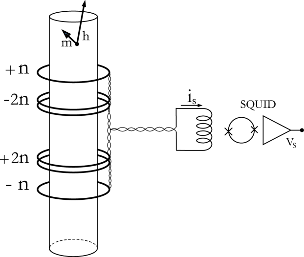
Figure 1: Schematic of the basic circuit for noise measurement. In order to maximise the coupling factor between the sample and the Pick Up coil, a long cylinder ($4\,\mathrm{cm}$ long, $4\,\mathrm{mm}$ wide) is used. The third order gradiometer being $2.2\,\mathrm{cm}$ long $5.5\,\mathrm{mm}$ wide, this size insures almost the best possible coupling factor, as any contact between the PU-coil and the sample must be avoid to allow the temperature regulation.

The protocol of spontaneous magnetic fluctuations measurements is quite simple: a thermalised sample is introduced in a pick-up coil (PU), itself part of a superconductive circuit involving the input coil of a SQUID-based flux detector (see Fig. 1).

Materially, the sample of cylindrical shape with diameter and length $5\,\mathrm{mm}$ and $40\,\mathrm{mm}$ respectively is contained in a cylindrical vacuum jacket, part of a ⁴He cryogenic equipment. The PU is wound on the jacket. The sample itself is contained in a cylinder made of copper coil-foil whose upper part is a copper sink with thermometer resistor and heater resistor, thermally connected to the ⁴He bath by a flexible copper link, thus allowing temperature regulation above $4.2\,\mathrm{K}$. The vacuum system involves a charcoal pump thermally connected to the ⁴He through a thermal impedance. When cold, it insures good thermal insulation; if heated, it allows to inject ⁴He exchange gas thus thermally connecting the whole sample to the helium bath temperature.

The difficulties of the measurement lie in the extreme weakness of the signal of the fluctuations and the strong response to external excitations: the typical amplitude of magnetic fluctuations in our macroscopic $\mathrm{CdCr_{1.7}In_{0.3}S_{4}}$ sample corresponds to the response to a magnetic field about $10^{-7}\,\mathrm{G}$. Several magnetic shields ($\mu$-metal and superconductive) are used in order to decrease the residual field at a level of order $1\,\mathrm{mG}$, and to stabilise it. Furthermore, the PU is built with a third order gradiometer geometry, which strongly reduces the sensitivity to the time variations of the ambient fields. In such conditions, and because of the extreme sensibility of SQUID measurements, a satisfactory signal/noise ratio can be easily obtained at short time-scales, corresponding to correlation measurements with time differences of few seconds. In order to study a glassy system in the deep ageing regime, such time-scales are not enough: one needs to measure the time autocorrelation with time differences up to several thousand seconds. To suppress spurious drifts of the measuring chain, further precautions are then needed: stabilisation of the helium bath to avoid drifts of the SQUIDS sensor, stabilisation of the room temperature to avoid drifts in the ambient temperature electronics, etc.

It should be emphasised that the use of the third order gradiometer in this experiment is quite different from the most common use. Usually, gradiometers are used in magnetometers where the sample is small compared to the gradiometer size, and is placed in a non-symmetric position; an homogeneous field is established, and the unbalanced flux due to the magnetisation of the sample is recorded.

2.2 Response measurements

Already several years ago, a comparative study of the magnetic fluctuations and the conventional magnetic response was done using a setup similar to the one schematically described in figure 1 Refregier00 . This comparison could not be made quantitative with a satisfactory accuracy: the coupling factor of the sample to the detection system depends on the PU geometry and is quite different in the noise setup and in a classical magnetometer with homogeneous field. In order to be able to compare quantitatively the results of both kinds of experiment, one has to eliminate the effect of this geometrical factor in the comparison. This can be done only if the coupling factor is the same in both experiments. The way to achieve this can be illustrated very simply. The fluctuations of the magnetisation are recorded through a PU coil with a given geometry. According to the reciprocity theorem, the flux fluctuations induced in the coil are the fluctuations of the scalar product of local magnetisation $\mathbf{M}\mathrm{dV}$ by the local field $\mathbf{h}$ produced by a unit of current flowing in the PU coil:

$$\Phi=\int_{sample}\mathbf{M}.\mathbf{h}\mathrm{dV}$$

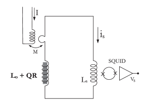
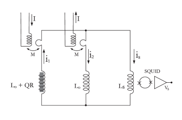
Figure 2: Schematic of the FDT circuits. Top : Basic FDT circuit. Bottom : The bridge configuration used.

In our setup, the measured fluctuating observable is the flux in the PU-coil. The conjugate quantity of this flux is the current flowing through the coil, and thus, the magnetic field conjugate of the sample magnetic moment is the field produced by the PU-coil itself. If this field is used as exciting field, then the fluctuation-dissipation relation should remain the same for the macroscopic quantities as for the microscopic ones. This is strongly different from the situation where one tries to compare the results of noise measurements to the results of classical response measurements done in an homogeneous field: then the coupling factor in both measurements has to be evaluated. A way to use the PU-coil as field generator is the following. A small coil coupled to an excitation winding with mutual inductance $M$ is inserted in the basic superconductive circuit (see Fig. 2.a).

2.3 Absolute thermometer

2.3.1 Fluctuation Dissipation relation

Here we will show that, for any given equilibrated system, the validity of FDT on microscopic quantities results in the validity of an “effective FDT” on measured quantities. The factor $K$ which appears is setup dependent, but sample independent.

When a magnetic sample is inserted into the PU coil, by the reciprocity theorem, a moment $\mathbf{m}_{i}$ at position $\mathbf{r}_{i}$ induces in the coil a flux $\delta\Phi=\mathbf{m}_{i}\mathbf{h}_{i}$ . Therefore, the flux in the coil due to the sample is given by

$$\Phi=\sum_{i}\sum_{\mu}m^{\mu}_{i}h^{\mu}_{i},$$ (3)

where $\mu$ indexes the spin components: $\mu=\{x,y,z\}$ for Heisenberg spins, $\mu=\{z\}$ for Ising ones, etc. We suppose that the medium is homogeneous, the components of the fluctuations are statistically independent and their spatial correlations are much smaller than the scale of the PU:

$$\left<m^{\mu}_{i}(t^{\prime})m^{\nu}_{j}(t)\right>=\left<m(t^{\prime})m(t)\right>\delta_{ij}\delta_{\mu\nu}.$$ (4)

Then, the flux autocorrelation is given by

$$\left<\Phi(t^{\prime})\Phi(t)\right>=\sum_{\mu}\sum_{i}{h^{\mu}_{i}}^{2}\left<m(t^{\prime})m(t)\right>=QC(t^{\prime},t).$$ (5)

The flux autocorrelation in the PU is thus the averaged one site moment autocorrelation per degree of freedom $C(t^{\prime},t)$, multiplied by the coupling factor $Q$ determined by the geometries of the PU field and of the sample.

On the other hand, the impulse response function of one moment in the sample is given by

$$R^{\mu\nu}_{ij}(t^{\prime},t)=\frac{\partial m^{\nu}_{j}}{\partial h^{\mu}_{i}}=R(t^{\prime},t)\delta_{ij}\delta_{\mu\nu},$$ (6)

where $R(t^{\prime},t)$ is the averaged one site response function of the sample. If a current $i$ is flowing in the coil, the flux on the coil due to the polarisation of the sample reads

$$\Phi(t)=\sum_{i}\sum_{\mu}{h^{\mu}_{i}}^{2}\int^{t}R(t^{\prime},t)i(t^{\prime})dt^{\prime}.$$ (7)

Thus, the response function of the flux due to the sample in the PU circuit is

$$R_{\Phi}(t^{\prime},t)=QR(t^{\prime},t).$$ (8)

The same coupling factor $Q=\sum_{i}\sum_{\mu}{h^{\mu}_{i}}^{2}$ determines the values of correlation and response of the flux due to the sample.

Note that the term $h$ is the value of the internal field in the sample, due to a unit of current flowing in the coil. Therefore, $Q$ corresponds to the same demagnetising field conditions in both measurements. Actually, $Q$ is time dependent, since the internal field is $h=h_{0}\mu(t^{\prime},t)$ where $h_{0}$ is the field term generated by the coil in vacuum and $\mu(t^{\prime},t)$ is the time dependent sample permeability, but the important point is that $Q(t^{\prime},t)$ is exactly the same in both experiments.

The above derivation is done in the context of a magnetic system, showing that the measured quantities represent those used in theoretical work, in which the single-site autocorrelation and response functions are computed, and averaged over the sample. Incidentally, an equivalent derivation could be done for any system with magnetic response, for instance the eddy currents in a conductor, with the same result: the coupling factors are the same in the fluctuations and the response measurements.

In the basic measurement circuit, Fig. 2.a, the total flux impulse response of the circuit to the current $i(t^{\prime})$ flowing in it is

$$R_{L}(t^{\prime},t)=\sum L\delta(t-t^{\prime})+Q(t^{\prime},t)R(t^{\prime},t),$$ (9)

where $\sum L$ is the total self inductance of the circuit. Flux conservation in the (SC) PU circuit leads to

$$\Phi_{exc}(t)+\int_{-\infty}^{t}R_{L}(t^{\prime},t)i(t^{\prime})dt^{\prime}=0,$$ (10)

where $\Phi_{exc}(t)=MI(t)$ is obtained by injecting a current $I(t)$ in the excitation winding. The conjugate variable of the circuit current $i$ is the flux $\Phi_{exc}$ injected by the excitation coil. In the case of an ergodic sample, it is easy to show that, once FDT applies to the fluctuations and response of the flux induced in the PU, it applies also to the fluctuations and response of the current flowing in the circuit. Thus,

$$\sigma_{i}(t-t^{\prime})=\frac{1}{k_{B}T}C_{i}(t-t^{\prime}).$$ (11)

The SQUID gain is $G=V_{S}/i$. Thus, if a current $I(t)=I_{0}(1-\theta(t))$ is injected in the excitation coil, the relaxation of the SQUID output voltage is related to the autocorrelation function of its fluctuations by:

$$V_{S}(t)=\frac{1}{KT}\left<V_{S}(0)V_{S}(t)\right>.$$ (12)

where $K=\frac{G}{MI_{0}}k_{B}\,$. The system is an absolute (primary) thermometer since, by measuring both the response voltage to an excitation current step and the autocorrelation of the voltage free fluctuations, it allows a determination of the temperature whose precision (once a sample with large signal is chosen) depends only on the precision of the determination of the experimental parameters $I_{0}$, $G$ and $M$.

The main drawback of the elementary measuring circuit depicted above is that the response to an excitation step involves the instantaneous response of the total self inductance of the circuit (first term in the right hand side —R.H.S— of Eq. 9). In our case, both the susceptibility of the sample and the coupling factor $Q$ are weak. The quantity to be measured,— the second term in the R.H.S of Eq. 9—, represents a few percent of the first one. Thus, a bridge configuration as depicted in Fig. 2.b has been adopted. Now, the main branch involving the sample is balanced by an equivalent one without sample. This second branch is excited oppositely, in such a way that when the sample is extracted from the PU, there is no response of the SQUID to an excitation step. When the sample is placed into the PU, the response of the SQUID is determined only by the response of the sample. Nevertheless, now, the loop coupling factor of the sample to the SQUID involves different self inductance terms in both measurements, and one gets

$$K=\frac{G}{MI_{0}}\frac{L_{0}+2L_{S}}{L_{0}}k_{B}$$ (13)

where $L_{0}$ and $L_{S}$ are the self inductances of the PU and of the SQUID input respectively, and the effect of the sample has been neglected in the value of $L_{0}$. This adds sources of error on the calibration since the self inductance values are difficult to determine precisely.

2.3.2 Calibration.

The circuit as described above is a thermometer, allowing the determination of the temperature, $k_{B}T$. Nevertheless, it involves several home-made coils whose self-inductances cannot be determined in their experimental environment without large errors. This dramatically limits the precision on the determination of the temperature. A calibration was thus needed. For this, the fluctuations and response of a high conductivity copper sample were measured in the setup. This high purity ($99,999\%$) sample has a very low residual resistivity at low temperature, obtained by annealing at high temperature in oxygen atmosphere, thus reducing the density of magnetic residual impurities. The sample has a cylinder shape, $5\,\mathrm{mm}$ wide and $4\,\mathrm{cm}$ long. It was thermalised at the temperature of the boiling ⁴He at normal pressure ($4.215\,\mathrm{K}$).

\psfrag{correlation1}[Bc][tc]{\scriptsize$C(\tau)$}\psfrag{correlation1}[Bc][tc]{\scriptsize$C(\tau)$}\psfrag{correlation}[cc][Bc]{\scriptsize Autocorrelation $C(\tau)$,$[\,\mathrm{V^{2}_{PP}}]$}\psfrag{relaxation}{\scriptsize$\sigma(\tau)$,$[\,\mathrm{V}]$}\psfrag{time}[cc][cc]{\scriptsize Observation time, $\tau$~{}$[\,\mathrm{s}]$}\includegraphics[width=203.80193pt]{./CuKuCu2bis}

Figure 3: Measured relaxation (a) and autocorrelation (b) function for the copper sample at $4.2\,\mathrm{K}$. (c) FD-plot, relaxation versus response, the observation time $\tau=t-t_{w}$ being used as parameter: the observed linear behaviour allows calibration of the system as thermometer, this slope being proportional to $1/T$, independently of the sample. The observed deviation from the linear behaviour at the shorter times is due to the effect of the low-pass filtering of the excitation— which does not affect the correlation measurement.

Since this equilibrated system is stationary, one can use standard Fast Fourier Transform algorithms in order to compute the autocorrelation function from a single record. The average of the obtained autocorrelation function over many successive records allows to reduce the noise level.

The relaxation function is obtained as the response to a field step at $t_{w}$, and is only a function of $t-t_{w}$. As the system does not have remanent magnetisation (the eddy currents vanish in a finite time, a few tenth of a second), the limit value of the response function is zero.

The measured relaxation and autocorrelation of SQUID voltage are plotted in figure 3(a) and (b) versus the observation time. The fluctuation-dissipation diagram (FD-plot) is obtained by plotting the relaxation versus autocorrelation, using the observation time as parameter, in figure 3(c) . The observed linear behaviour is consistent with the FDT. As previously shown, the slope between the relaxation and the response is sample-independent, and proportional to $1/KT$. The measurement on the copper sample, at a well known temperature allows thus to determine the factor $K$. From it, we can determine the temperature of any sample placed in the gradiometer from the value of the slope of the measured relaxation versus correlation curve. This can be applied to any equilibrated system. For glassy systems, it should allow an experimental determination of the effective temperature.

3 Fluctuation-dissipation relations in a spin-glass sample

The aim of this work is the study of the fluctuation-dissipation relation in a spin glass. In this section, we will emphasise the peculiarities of this measurement, and then describe the procedure used to make the analysis quantitative as well as the limits of this procedure.

3.1 Sample

The knowledge acquired in previous magnetic noise investigations on spin glasses was very helpful to choose a good candidate for the present study. First, eddy currents in metallic samples produce noise, as in the copper sample used for calibration. This noise can be measured, but not directly related to the spin dynamics. In order to avoid this drawback, an insulating spin glass sample was chosen.

Measurements on $\mathrm{CsNiFeF_{6}}$ have shown that this compound has a stronger signal, and then a better signal to noise ratio than any other insulating spin glass refregier04 . Nevertheless it has a very strong ferromagnetic value of the average interaction and its behaviour is far from the “standard” spin glass behaviour.

$\mathrm{CdCr_{2-2x}In_{2x}S_{4}}$ was also extensively studied experimentally, by classical susceptibility, magnetic noise, neutron scattering Alba01 ; Albath ; Alba02 ; Pouget02 . In this series of compounds, the magnetic ions are $\mathrm{Cr^{3+}}$, with low anisotropy. The coupling is ferromagnetic between first neighbours, and anti-ferromagnetic between the second ones. The substitution of $\mathrm{Cr^{3+}}$ by the non-magnetic $\mathrm{In^{3+}}$ increases the relative importance of anti-ferromagnetic coupling as compared to the ferromagnetic one. The random dilution introduces disorder and frustration, the basic ingredients leading to spin-glasses. In the studies of the spin glass state, $\mathrm{CdCr_{1.7}In_{0.3}S_{4}}$ is the preferred compound in this family. The high concentration of $\mathrm{Cr^{3+}}$ allows this sample to have a strong signal, but it is not high enough to reach the percolation of the ferromagnetic order. With decreasing temperature, finite sized ferromagnetic cluster formation is observed. Close to $T_{g}$, these clusters are rigid, and the interaction between them is random, with a weak anti-ferromagnetic average. This clustering greatly increases the signal, as the noise power of $N=N_{0}/n$ ferromagnetic clusters of $n$ spins is $\sqrt{n}$ times stronger than the one of $N_{0}$ individuals spins.

3.2 Experimental details

Glassy systems are not stationary; their dynamics depends on two times, both referred to a crucial event, the “birth” of the system. In spin glasses, the birth time is best defined by the time at which the final temperature is reached, as soon as the end of the cooling procedure is fast enough Jonason00 . A cooling procedure based only on driving the sample holder sink temperature would introduces non-negligible temperature gradients if the cooling or heating rate is too high. This would lead to a distribution of ages over the sample. In order to obtain a more homogeneous temperature, the cooling procedure is as follows:

• first, the temperature is slowly decreased from a reference temperature $T_{ref}$ above $T_{g}$ to a temperature $T_{1}\approx T_{m}+3\,\mathrm{K}$, where $T_{m}$ is the working temperature;

• then, by heating the charcoal pump, a small amount of He gas is introduced, allowing a quick and homogeneous cooling;

• finally, the charcoal pump heating is switched off and the vacuum surrounding the sample is restored, allowing the temperature regulation at $T_{m}$.

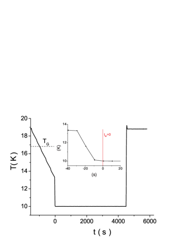
Figure 4: A typical thermal history of the sample for a $4,500\,\mathrm{s}$record at $10\,\mathrm{K}$. In inset, detail on the crucial part, the last $3\,\mathrm{K}$’s cooling.

The first step (slow cooling, approx. $0.25\,\mathrm{K.min^{-1}}$) does not introduce severe temperature gradients, as the cooling is slow enough. This step cannot be avoided, as the fast cooling by exchange gas can only be used to decrease the sample temperature by few Kelvin without introducing too strong perturbations in the helium bath. Previous studies on $\mathrm{CdCr_{2-2x}In_{2x}S_{4}}$ show that the dynamics is governed by the second, fast, cooling step, at least on timescales shorter than $20,000\,\mathrm{s}$ Jonason00 . This second step is obtained by heating the charcoal pump during few seconds. As the gas surrounds the sample, the resulting cooling is homogeneous. When the heating is stopped, the charcoal absorbs the gas back, allowing the regulation of temperature. The amount of gas used and the duration of heating are adjusted in order to lower the temperature exactly down to the working temperature. This allows to cool the sample by $3\,\mathrm{K}$ in less than $30\,\mathrm{s}$, keeping the temperature gradient negligible. The birth time is taken as the instant when the sample temperature reaches $T_{m}+15\,\mathrm{mK}$. This allows a precise, and reproducible determination of it.

The measurement of the relaxation is straightforward. A DC current is applied to the excitation coils at high temperature, before the beginning of the quench procedure, and switched off at $t=t_{w}$. The relaxation is then recorded for $t>t_{w}$. The signal is measured before applying the excitation: this determines the zero baseline of the measurement. After relaxation, the sample is re-heated to the start temperature in order to check the stability of the baseline. Thus, in the measurement, both the zero and field cooled (FC) levels are known.

Recording the fluctuations is even simpler, at least in principle: no field is applied, the spontaneous fluctuations of the signal are just recorded from the end of the quench procedure and during a long enough time to be able to compute all the desired $C(t_{w},t)$. However, as the system is not ergodic in the ageing regime, the autocorrelation of the signal cannot be evaluated from a single record, as for an equilibrated sample. In order to compute the autocorrelation function, an ensemble average has to be done on successive equivalent records, each one initiated by a quench. This does not only increase dramatically the length of the experiment, but also the difficulties of the acquisition, the ideal acquisition conditions having to be kept during months instead of hours. This complication has nevertheless an advantage: by averaging, it allows to make the separation between a systematic spurious signal and the signal of the fluctuations. In our results, the systematic signal is of the same order of magnitude as the fluctuations themselves. It corresponds to the drift of the SQUID due to the continuous decrease of the He-level, and to the global response of the sample to the residual field during the cooling procedure. The average of the signal over records gives the zero, and the sample fluctuations signal is then given by:

$$m(t)=M(t)-\left<M(t)\right>$$ (14)

The autocorrelation is then evaluated from its definition:

$$C_{1}(t,t_{w})=\left<m(t_{w})m(t)\right>$$ (15)

In order to obtain a small statistical error, a very huge number of records is needed. As each record length is about few hours, the number of records is limited to about 300, and the average over the records is not enough to obtain a satisfactory ratio between the statistical error and the signal. As the autocorrelation function should evolves smoothly for both variables, $t_{w}$ and $t$, the autocorrelation function computed following eq. 15 is averaged over small time intervals of both variables :

$$C_{avg}(t_{0},t_{w_{0}})=\overline{C_{1}(t,t_{w})}|_{t_{w}\in[t_{w_{0}}\pm\epsilon_{t_{w_{0}}}],\,t\in[t_{0}\pm\epsilon_{t_{0}}]}$$ (16)

with

$$\epsilon_{t}=0.05t\ll t.$$ (17)

The criterion used (Eq. 17) is a compromise between the need of statistics in order to obtain a low enough statistical noise, and the requirement to keep $\epsilon$ as small as possible to be able to capture as precisely as possible the non-equilibrium dynamics.

3.3 Correlation offset.

In principle, our experimental procedure, involving many realisations of the same experiment, allows to compute the autocorrelation function of the magnetisation following its exact definition, and thus exactly. Nevertheless, in reality, this would be the case only if external sources of noise were negligible, not only in the correlation time-scale under study, but also in the time-scale of one complete record. This means that the external noise should be controlled not down to $1\,\mathrm{mHz}$ as in our experiment, but at least down to frequencies as low as few $0.01\,\mathrm{mHz}$, which is quite impossible. The result is that the computed correlation $C(t_{w},t-t_{w})$ contains an offset practically independent on $t-t_{w}$ but randomly dependent on $t_{w}$.

As the setup is a calibrated thermometer, the temperature can be extracted from the derivative of the $\chi(C)$ curves in experimental units. In order to obtain the FD-plot, this is not enough. For a normalisation of the data, one needs to know the zero reference level of the response and of the correlation. In the case of the copper sample data, where the eddy currents producing the signal have a finite and experimentally accessible lifetime, this calibration is trivial: relaxation and autocorrelation functions decrease to zero after a few seconds. In the spin glass case, normalisation of the relaxation is simple since the zero level and the FC level are determined during the measurement. For the correlation, things are not so easy.

As seen above, at a given temperature, the correlation curves for different $t_{w}$ are shifted between each other by a random unknown offset. Nevertheless, it is possible to normalise the data by taking as the origin of each curve the square of the measured value of the first point, $C_{avg}(t_{w},t_{w})$. Due to the elementary measurement time constant, this term corresponds to an average over $t-t^{\prime}$ about $10^{-2}\,\mathrm{s}$, i.e., a range of $(t-t^{\prime})/t^{\prime}$ corresponding to the stationary regime where all curves must merge. Thus, the following quantity is computed:

$$C(t,t_{w})-C_{0}=C_{avg}(t,t_{w})-C_{avg}(t_{w},t_{w})$$

The “individual” offset is now replaced by a “global” one, $C_{0}$, which should apply simultaneously to any measurement done at a given temperature.

Then, the best way to normalise our data could be to extract $C(t,t)$ from some other measurement, and to be able to convert it in the “experimental units”. Neutron diffraction experiments are now under way in order to measure this quantity. $C(t,t)$ can also be extrapolated from high temperature measurements (above $T_{g}$) to low temperatures (below $T_{g}$), or deduced from some other quantities. Then a complete —but model-dependent— determination of the autocorrelation can be obtained, allowing to obtain the FD-plot. Anyway, even if the hypothesis used to obtain this complete determination of the autocorrelation were not realistic, some characteristics of the FD-plot would not be affected. The temperatures, effective or not, are measured from the slope between relaxation and correlation in the experimental units. They will not be modified by the normalisation procedure, whose effect is just to suppress an offset.

4 Discussion

In this section, the results of the measurements done at several temperatures in $\mathrm{CdCr_{1.7}In_{0.3}S_{4}}$ will be analysed following the line of the method described above.

4.1 Raw measurement

Figure 5 displays the values of $\chi(t_{w},t)/\chi_{FC}=1-\sigma(t_{w},t)/\chi_{FC}$ plotted versus $C(t_{w},t)$ for several values of $t_{w}$ and using $t-t_{w}$ as parameter. The three graphs correspond to the three temperatures 10, 13.3 and $15\,\mathrm{K}$. A first observation is that a linear regime exists between relaxation and correlation for all the temperatures and waiting-time investigated. This regime corresponds to the shorter observation times. In the figures, the straight lines represent the FDT slope as calculated from the values of calibration factor $K$ and of the temperature: in this regime, the relation between relaxation and correlation follows the FDT. Thus, this regime can be extrapolated from the shorter experimental observation-time down to the microscopic time-scale. This extrapolation at short time should reach the starting point of the FD-plot: $C(t_{w},t_{w})$ corresponds to $\chi(t_{w},t_{w})=0$. As no long term memory is observed in spin-glasses, $C(t_{w},+\infty)=0$ should also correspond to $\chi(t_{w},+\infty)=\chi_{FC}$, but the extrapolation to this point is not obvious at all, as the (unknown) ageing regime should be extrapolated.

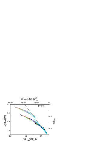
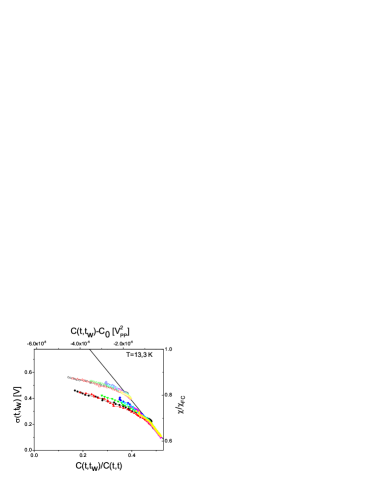
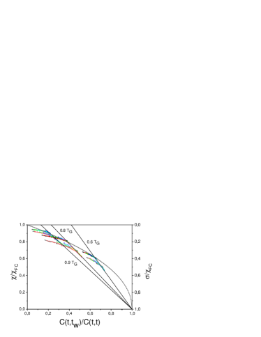
Figure 5: Raw results (full symbols) and ageing part (open symbols) deduced from the scaling analysis for the three investigated temperature, $T=10,13.3,15\,\mathrm{K}$. The straight lines have the FDT-slope obtained from the copper calibration for each temperature of the formalisation bath, and start all from the point $(\sigma/\chi_{FC}=1,C/C(t,t)=1)$. The correlation offset is adjusted following the “PaT hypothesis” (cf section 4.3.3) The different curves span the waiting times studied: $\circ:t_{w}=100\,\mathrm{s},\,{\color[rgb]{1,0,0}\triangle}:t_{w}=200\,\mathrm{s},\,{\color[rgb]{0,1,0}\triangledown}:t_{w}=500\,\mathrm{s},\,{\color[rgb]{0,0,1}\diamond}:t_{w}=1000\,\mathrm{s},\,{\color[rgb]{0,1,1}\triangleleft}:t_{w}=2000\,\mathrm{s}$ and, only for $T=13.3\,\mathrm{K}$, ${\color[rgb]{1,0,1}\triangleright}:t_{w}=5000\,\mathrm{s},\,{\color[rgb]{1,1,0}\circ}:t_{w}=10000\,\mathrm{s}$.The last plot represent the complete FD-plot for each previous measurement measurements reported on the same graph, the smooth curve corresponds to equation 26, with an exponent $B=0.47$.

4.2 Scaling procedure

The raw results show a waiting time dependence which can be easily explained. The main theoretical predictions correspond to the approach of the limit $t_{w}\rightarrow\infty,\,C(t_{w},t)=C$ (WEB). In this case, the stationary and the ageing parts of the dynamics evolve on distinct time-scales, yielding a separation of both dynamics. Experimentally, such a separation is not accessible since the waiting times are finite. In order to separate both part of the dynamics, the entanglement between both part should be described. The simplest way to combine these two contributions is to add them. For instance, if one considers the relaxation $\sigma$ observed after a unitary field step at time $t_{w}$:

$$\sigma(t_{w},t)=(1-\Delta).\sigma_{stat}(t-t_{w})+$$

$$\Delta.\sigma_{ageing}\left(\lambda(t)-\lambda(t_{w})\right)$$ (18)

In this equation, all the different $\sigma$ are normalised to unity. This relation is obviously valid in the limit of separation of time-scales, and is the most commonly used in theoretical approaches, but it is counter-intuitive as shown by the following two thought-experiments:

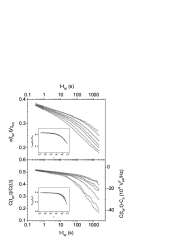
Figure 6: Relaxation (Top) and autocorrelation (Bottom) functions recorded at $13.3\,\mathrm{K}$. The different curves correspond, from bottom to top, to $t_{w}=100$, 200, 500, 1 000, 2 000, 5 000 and $10\,000\,\mathrm{s}$. In insets, the respective ageing parts, deduced by the scaling analysis developed in section 4.2

• In the first one, a glassy system is quenched at a temperature below $T_{g}$ at time $t=0$, and at $t=0^{+}$, a field is applied. This experiment is usually though as being equivalent to the “Field-cooled” procedure, in which the field is applied before the quench. Experimentally, the Field Cooled magnetisation is strikingly stable. In the additive formulation, the predicted behaviour is the following: first, an instantaneous variation due to the ageing part, and then a slow variation up to the FC value, as the system approaches equilibrium. Thus, the field-cooled magnetisation should not be as stable in time, as what is observed experimentally.

• The second problem arises when thinking about some finite $t_{w}$ experiments, but with (very) huge time differences, $t\rightarrow\infty$. Ageing and stationary parts are usually described as stretched exponential (with characteristic time of order $t_{w}$) and power-law with small exponent respectively. For finite $t_{w}$, after a finite time, the only remaining contribution to the dynamics would come from the stationary part, and FDT would be recovered.

If the time-scales are not well separated, it seems intuitively that the two different contributions must be more entangled than the result of a simple addition. Another (more realistic) way to mix the two parts together is to consider a “multiplicative” combination, which can be written as:

$$\sigma(t_{w},t)=\left[(1-\Delta).\sigma_{stat}(t-t_{w})+\Delta\right]\times$$

$$\sigma_{ageing}\left(\lambda(t)-\lambda(t_{w})\right)$$ (19)

In the limit of time-scales separation, equations 18 and 19 are equivalent. Moreover, it is easy to show that the problems raised in the two cases discussed above disappear. Thus, as this formulation is at least as justified as the “additive” one, and seems less counter-intuitive to the authors, it will be preferred in the following.

Experimentally, separation of timescales is not accessible since the waiting times are finite. In order to separate both part of the dynamics, a scaling analysis, as described by equation 19 and illustrated by Fig. 6 is applied on both relaxation and correlation measurements, within the following constraints:

1. In the relaxation, the stationary part is described by a power-law decay; its exponent $\alpha$ is extracted from the decay of the noise power-spectra measured on the same sample, at the same temperature, in the quasi-equilibrium regime obtained after a very long waiting at the working temperature (typically 15 days) Refregier03 .

2. In the non-stationary regime, the effective time is given by $\lambda=\frac{t^{1-\mu}}{1-\mu}$. The value of the sub-ageing exponent, i.e., $\mu$ is in the range $0.85-0.9$ Alba01 . $\mu$ and the relative amplitude of the ageing part, i.e., $\Delta$, are chosen to obtain the best rescaling of the relaxation curves once the stationary part has been subtracted.

3. The stationary part of the autocorrelation function is then evaluated using FDT and the stationary part of the relaxation. The ageing part of the autocorrelation can then be deduced from equation 18 or 19.

The resulting FD-plots are displayed in open symbols in the diagrams of figure 5 for the ageing part (by construction, the stationary part follows the FDT line). For all the investigated temperatures, the ageing part starts with a slope very close to the FDT one. This may reflect the imperfections of our decomposition between the stationary and the ageing parts. Using the additive scaling, this effect is even more pronounced.

The multiplicative scaling has a main drawback: it can not be used without the knowledge of the amplitude of the concerned physical quantity. As previously discussed in section 3.3, for the correlation this value must be determined indirectly, and is model dependent; thus the scaling is also model-dependent. The additive form of the scaling can be applied without any amplitude parameter. However, the dependence of the scaling on this parameter is weak, the results obtained from different models are indistinguishable from each other.

The ageing part of the correlation function is found to follow remarkably the scaling-law used for the ageing part of the response, resulting in a very weak systematic $t_{w}$-dependence of the FD-plots. Thus, the equation 18 (or 19) can be written for the correlation, with the amplitude parameter $\Delta$ replaced by $q_{EA}$, the usual Edwards-Anderson order parameter EA , which is defined as the remaining part of the autocorrelation for an equilibrated spin glass after an infinite waiting time. As a consequence, the FD-plots are determined by a single parameter, the effective time difference: the limit FD-plots, corresponding to the ideal separation of the stationary and ageing regime is independent of the age of the system, as supposed in theoretical works.

4.3 Comparisons with some models predictions

Depending on the models, some remarkable features of the FD-diagrams are predicted. The analysis of the FD-diagrams may help to check the validity of the models used to interpret the glassy behaviour found in $\mathrm{CdCr_{1.7}In_{0.3}S_{4}}$.

4.3.1 Domain growth

In domain growth models, as in any replica symmetric models, the FD-plot should be quite simple in the limit of time-scale separation. For an infinite waiting time $t_{w}$, the quasi-equilibrium relaxation should go down to zero. A FDT-behaviour should then describe all the response, governed by the single-domain response and the scaling approach used in this paper should give $(q_{EA}\neq 0,\Delta=0)$. Thus, the remaining part of the diagram, an horizontal line, should correspond to an infinite effective temperature Barrat02 ; Corberi00 . This description does not coincide with the FD-diagram shown in figure 5, even after the separation of time-scales obtained by scaling.

Anyway, a more refined approach as in Yoshino00 is not excluded, in which dynamics is described introducing a crossover region in between the quasi-equilibrium region ($C>q_{EA}$) and a purely ageing region characterised “dynamical order parameter” $q_{D}$ for $C<q_{D}<q_{EA}$. This approach could explain the “early” departure from the FDT regime. This departure should be $t_{w}$-dependent, but this dependence may be hidden by a too small range of waiting times explored (as well as a too weak exploration of the ageing regime).

4.3.2 1-step replica symmetry breaking

In $\mathrm{CdCr_{1.7}In_{0.3}S_{4}}$, one of the best realisation of an Heisenberg spin-glass, it has been shown that the scenario of the chiral spin glass could be relevant Petit00 ; Petit01 . Such model belongs to the 1-step replica symmetry breaking (1-RSB) models family Kawamura02 ; Kawamura03 ; Hukushima00 .

In 1-RSB case, the ageing regime is described by a unique effective temperature, finite and strictly greater than the thermalisation temperature. By considering a normalised FD-plot, it is easy to show that the value of $q_{EA}$ can be deduced from the value of $T$, $T_{eff}$ and $\gamma={1-\Delta\over\Delta}$, the ratio between the stationary and the ageing part of the relaxation, which is experimentally accessible:

$$q_{EA}=\frac{1}{1+\gamma.{T\over T_{eff}}}$$ (20)

$T\,[\,\mathrm{K}]$	$T_{eff}\,[\,\mathrm{K}]$	$q_{EA}^{1-step}$	$q_{EA}^{PaT}$
10	$28\pm 6$	$0.65\pm 0.05$	0.63
13.3	$50\pm 10$	$0.45\pm 0.05$	0.37
15	$80\pm 20$	$0.36\pm 0.07$	0.21

Table 1: Values of $T_{eff}$ as obtained in an 1-step replica symmetry breaking scenario and the corresponding Edwards-Anderson order parameter $q_{EA}^{1-step}$ (cf section 4.3.2). The values of $q_{EA}^{PaT}$ are deduced from the PaT ansatz (cf. section 4.3.3).

As the experimental setup is a calibrated thermometer, it allows an absolute determination of the temperatures. The determination of $T$ and $T_{eff}$ extracted from the slope of the stationary and the ageing part respectively allows the complete determination of the offset $C_{o}$. The obtained values of $T_{eff}$ and $q_{EA}$ are reported in table 1. The separation by scaling between stationary and ageing part being far from perfect, the uncertainty on the determination of $T_{eff}$, and consequently on $q_{EA}$ is quite large. The choice of a scaling procedure also influences the results (the previously reported value for $T_{eff}\approx 30\,\mathrm{K}$ for a thermalisation temperature of $13.3\,\mathrm{K}$ was obtained by an additive scaling analysis of the data herisson00 ). The results of table 1 can be compared with the results of simulations done on a weakly anisotropic spin glass model by Kawamura Kawamura09 . In this work, it was found that $\chi$ depends linearly on $C$ in the ageing regime. The effective temperature was found to be independent of the temperature of the thermalisation bath. This independence does not appear in our data, but, maybe, it can be due to the extremely low anisotropy used in the simulations. $\mathrm{CdCr_{1.7}In_{0.3}S_{4}}$ is known to be an Heisenberg spin glass with a non negligible anisotropy, which as been found to be five times stronger than in the canonical $\mathrm{Ag\underline{Mn}}$ spin glass.

4.3.3 Continuous replica symmetry breaking

In continuous replica symmetry breaking ($\infty$-RSB) models, as the Sherrington-Kirkpatrick (SK) model SK ; SKb , the Parisi order parameter is a continuous function between 0 and $q_{EA}$ SGTAB ; replica3 . Links between statics and dynamics imply that the corresponding effective temperature is a smooth and not trivial function of the autocorrelation :

$$\frac{1}{T_{eff}}(\mathscr{C})=\frac{1}{T}\int_{0}^{\mathscr{C}}P(q)\mathrm{d}q$$ (21)

Then there is no trivial relationship between $q_{EA}$ and the measured quantities. It is nevertheless possible to to progress further if the studied compound is a canonical spin-glass. In these systems, the FC susceptibility is purely paramagnetic at high temperature, following equation 22, and below $T_{g}$, its value is temperature independent:

$$\chi_{FC}(T>T_{g})=C(t,t)/k_{B}T$$ (22)

$$\chi_{FC}(T<T_{g})=C(t,t)/k_{B}T_{g}$$ (23)

The lower the concentration of magnetic ions in the canonical sample, the smaller the probability of spins clustering and the better the validity of the above relations nagata00 . Thus, the value of $C(t,t)$ can be straightforwardly derived from susceptibility data. The canonical behaviour is also observed or imposed in theoretical models, and known as the Parisi-Toulouse Hypothesis PaT . This “PaT” hypothesis implies that the FC response is temperature independent, as observed in diluted spin glasses.

In samples with high concentration in magnetic sites, deviations from the simple canonical behaviour are observed, as well as the formation of clusters of spins. At low temperatures,the response of single spins is no more observed, but the response of some rigidly coupled groups of spins. For macroscopic quantities, this is equivalent to the response of fewer renormalised spins. In $\mathrm{CdCr_{1.7}In_{0.3}S_{4}}$, which has a mean coupling constant strongly ferromagnetic ($\Theta=100\,\mathrm{K}$ Albath ; Pouget00 ), this clustering may explain that at low temperature, but above $T_{g}$, the compound behaves as a compound with antiferromagnetic average of couplings. A standard Curie-Weiss law description around $30\,\mathrm{K}$ gives a mean coupling characterised by $\Theta\approx-9\,\mathrm{K}$ alba00 . Such a description, with a non-trivial $\Theta(T)$ variation, should be associated with a non-trivial, but still smooth, function $C(t,t;T)$. As informations on the variations of $C(t,t;T)$ are lacking we propose to consider that relations 22 and 23 are still valid in the general case. This is a strong hypothesis since it amounts to consider that the temperature variation of $\chi_{FC}$ is due only to the temperature variation of ${C(t,t;T)}$. One can write:

$$\frac{C(t,t;T)}{k_{B}T}=\chi_{FC}(T<T_{g})\frac{T_{g}^{*}}{T}$$ (24)

A smooth behaviour of $C(t,t;T)/k_{B}T$ around $T_{g}$ can be obtained using $T_{g}^{*}=17.2\,\mathrm{K}$ in the formula .

This ansatz gives an access to the unknown offset of the autocorrelation: i) the starting point of the FD-plot, corresponding to $[C(t_{w},t_{w};T);\,\sigma(t_{w},t_{w})]$ is completely defined, ii) $C(t_{w},\infty;T)$ corresponds to the point where the FDT line reaches the level given by $\chi_{FC}(T<T_{g})\frac{T_{g}^{*}}{T}$. Then the FD-graph can be plotted in reduced units as displayed in figure 5d. In this plot, the starting point ($C=1$) and the end point ($C=0$) are temperature independent. Furthermore, it has been shown (for some mean field models, and approximately for the SK model) that not only these points but also all the ageing part of the plot is temperature independent Cugliandolo17 . It is conjectured that this can be still valid in short range models Franz02 ; Marinari00 ; Marinari02 . This property is particularly interesting: it allows, by measurements at several temperatures, to obtain the whole “master” curve describing the ageing behaviour, even if each set of data spans a limited portion of the correlation. This feature has been already used to obtain the master curve from response data, assuming that the separation of time-scales is reached in usual susceptibility measurements Cugliandolo00 ; Zotev01 .

In the SK model at small $C$, it can be shown that the master curve should behave as Marinari00 :

$$\chi(C)=\sqrt{1-C}$$ (25)

For correlations close to zero, the slope of the FD-plot, $X(C)=\int_{0}^{C}{P(q)}\mathrm{d}q$, should asymptotically reach zero, as $P(0)$ is known to have a finite value in the continuous RSB case.

Equation 25 can be generalised by allowing any exponent different from $0.5$:

$$\chi(C)=(1-C)^{B}$$ (26)

Such a curve can be easily superimposed to our experimental results. Using a coefficient $B=0.47$, a single curve can describe the ageing regime at all the investigated temperatures and for the data close to $q_{EA}(T)$. Both the value of $q_{EA}(T)$ and the effective temperature close to $q_{EA}$ seem to be well described by Eq. 26.

For $C\ll q_{EA}$, at each temperature, the experimental points deviate from relation 26. This cannot be due only to the smaller signal to noise ratio at the longest timescales, since the effect seems to be more pronounced at the highest temperature, where the sample signal is the strongest.

A possible explanation is that the scenario with continuous replica symmetry breaking should be associated with a continuous distribution of timescales describing the system. As the limit of separation of timescales is not reached in our results, the ageing regime itself is a combination of many timescales. The scaling procedure allows to extract the stationary part, but not to reach the limit where a full time-scale separation is achieved.

A way to reach the limit could be to iterate the scaling procedure on the ageing data to separate the “ageing timescales”. The ageing regime can be considered as a pseudo-FDT one, with a temperature equal to $T_{eff}(q_{EA})$. Such a work on the available data is however hopeless, as the separation between stationary and ageing part seems obviously already far from perfect.

A scaling can be deduced from equation 26 Marinari00 , which, using $\Phi={1\over 1-B}$, can be written as, :

$$\chi.T^{1-\phi}=\left\{\begin{array}[]{ll}A[(1-C)T^{-\Phi}]^{B}&{\rm for}\;\;C\leq q_{EA}(T)\ ,\\ (1-C)T^{-\Phi}&{\rm for}\;\;C>q_{EA}(T)\ .\end{array}\right.$$ (27)

If a power-law can describe the ageing dynamics, then all the scaled data should merge along a single line. The best result is obtained for $B=0.5$, but the cloud of points remains very broad, and is not well described by the predicted straight-line in the $\log(T^{1-\Phi}\chi)$ vs $\log\left(T^{-\Phi}(1-C)\right)$ diagram.

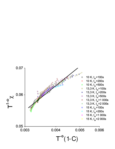
Figure 7: Scaling of the ageing parts of the FDT-diagram following equation 27. The straight line shows the result predicted by this equation.

5 Conclusion

In this paper, it has been shown that the experimental setup developed in this work can be considered as an absolute magnetic thermometer. However, to get rid of uncertainties on the value of several elements of the setup, the setup was calibrated by measuring the magnetic fluctuations and response of a high conductivity copper sample thermalised at helium temperature. This calibrated thermometer was used to determine the out-of-equilibrium properties of a spin-glass below the glass transition. The autocorrelation function of the spontaneous magnetic fluctuations of a well characterised insulating spin-glass was investigated in the deeply non-stationary regime. Its waiting time dependence can be described by using the same scaling as for the response function. The FD-plots clearly confirm that the stationary dynamics observed at the shorter timescales can be considered as a quasi-equilibrium once, as the fluctuation-dissipation relation between autocorrelation and relaxation obeys the fluctuation-dissipation theorem. The results show clearly that the asymptotic regime, with full separation of timescale is not reached. Certain Hypotheses on the dynamics are made in order to compare the results with model predictions. The deduced scaling analysis allows to extrapolate the experimental results to the limit used in theoretical studies of weak-ergodicity breaking models.

The experimental results obtained on $\mathrm{CdCr_{1.7}In_{0.3}S_{4}}$ differ qualitatively from the predictions of any domain-growth model.

The experimental data allow interpretations that are rather consistent with predictions from the two replica symmetry breaking models under study. As long as the autocorrelation cannot be determined completely, both models can be relevant, giving slightly different results concerning the value of $q_{EA}$. An independent determination of the characteristic magnetic moment of the clusters as a function of temperature is needed in order to resolve this ambiguity .

The possibility of analysing the experimental results on the basis of 1-step replica symmetry breaking confirms that, at first sight, the chiral model developed by Kawamura could be the more relevant one for the $\mathrm{CdCr_{1.7}In_{0.3}S_{4}}$compound with low anisotropy, supporting the conclusion from D. Petit and I. Campbell on this sample Petit00 . However, the scatter of the data is such that one cannot reject definitely an interpretation inspired by the mean-field models developed for Ising spin-glasses.

6 Acknowledgements

DH has been supported by the European Research Training Network Dyglagemem during the writting of this article. We thank G. Parisi for fruitfull discussions and Per Nordblad for a critical reading of the manuscript.

References

- [1] L.C.E. Struik. Physical Aging in Amorphous Polymers and Other Materials. Elsevier, Amsterdam, 1978.
- [2] J.A. Mydosh. Spin Glasses — An Experimental introduction. Taylor & Francis, London, 1993.
- [3] L.F. Cugliandolo and J. Kurchan. Analytical solution of the off-equilibrium dynamics of a long-range spin-glass model. Physical Review Letters, 71(1):173–176, July 1993.
- [4] L.F. Cugliandolo and J. Kurchan. On the out-of-equilibrium relaxation of the Sherrington-Kirkpatrick model. Journal of Physics A: Mathematical and General, 27:5749–5772, March 1994.
- [5] L.F. Cugliandolo, J. Kurchan, and L. Peliti. Energy flow, partial equilibration and effective temperatures in systems with slow dynamics. Physical Review E (Statistical, Nonlinear, and Soft Matter Physics), 55(4):3898–3914, April 1997.
- [6] H.B. Callen and T.A. Welton. Irreversibility and generalized noise. Physical Review, 83:34–40, July 1951.
- [7] R. Kubo. The fluctuation-dissipation theorem. Report on Progress in Physics, 29:255, 1966.
- [8] T.S. Grigera and N.E. Israeloff. Observation of fluctuation-dissipation theorem violations in a structural glass. Physical Review Letters, 83(24):5038–5041, December 1999.
- [9] L. Bellon, S. Ciliberto, and C. Laroche. Fluctuation-dissipation theorem violation during the formation of a colloïdal-glass. Europhysics Letters, 53(4):511–517, 2001. cond-mat/0008160.
- [10] L. Bellon and S. Ciliberto. Experimental study of fluctuation-dissipation-relation during an aging process. Physica D, 168–169:325–335, 2002. cond-mat/0201224.
- [11] J.-P. Bouchaud, E. Vincent, and J. Hammann. Towards an experimental determination of the number of metastable states in spin-glasses? Journal de Physique I—France, 4(1):139–145, January 1994.
- [12] B. Derrida. A generalization of the random energy model which includes correlations between energies. Journal de Physique Lettres—Paris, 46:L401–L407, 1985.
- [13] E. Vincent, J. Hammann, M. Ocio, J-P. Bouchaud, and L.F. Cugliandolo. Slow dynamics and aging in spin glasses. In E. Rub, editor, Proceedings of the Sitges conference on Complex Behaviour of Glassy Systems, June 1996. cond-mat/9607224.
- [14] Ph. Réfrégier, M. Ocio, J. Hammann, and E. Vincent. Nonstationary spin glass dynamics from susceptibility and noise measurements. Journal of Applied Physics, 63(8):4343–4345, April 1988.
- [15] P. Réfrégier, M. Alba, J. Hammann, and M. Ocio. Dynamic behaviour of the insulating spin glass . Journal of Physics C: Solid State Physics, 20:5545–5555, November 1987.
- [16] M. Alba, J. Hammann, M. Ocio, Ph. Réfrégier, and H. Bouchiat. Spin-glass dynamics from magnetic noise, relaxation, and susceptibility measurements (invited). Journal of Applied Physics, 61(8):3683–3688, April 1987.
- [17] M. Alba. Recherche et Etude de Phases Verre de Spins dans les Spinelles de Chrome Diluées : et . PhD thesis, Université de Paris XI, Orsay, 1982.
- [18] M. Alba and S. Pouget. Dynamic critical behavior of disordered 3D Heisenberg ferromagnets. In Journal of Magnetism and Magnetic Materials, volume 226-230, pages 542–4, May 2001.
- [19] S. Pouget and M. Alba. Spin arrangements in -type insulating re-entrant compounds. Journal of Physics: Condensed Matter, 7(24):4739–49, June 1995.
- [20] K. Jonason, E. Vincent, J. Hammann, J-P. Bouchaud, and P. Nordblad. Memory and chaos effects in spin glasses. Physical Review Letters, 81(15):3243–3246, October 1998.
- [21] Ph. Réfrégier, M. Ocio, and H. Bouchiat. Equilibrium magnetic fluctuations in spin glasses: Temperature dependence and deviations from 1/f behaviour. Europhysics Letters, 3(4):503–510, February 1987.
- [22] S.F. Edwards and P.W. Anderson. Theory of spin glasses. Journal of Physics F: Metallurgic Physics, 5:965–974, May 1975.
- [23] A. Barrat. Monte carlo simulations of the violation of the fluctuation-dissipation theorem in domain growth processes. Physical Review E, 57(3):3629–3632, March 1998.
- [24] F. Corberi, E. Lippiello, and M. Zannetti. Interface fluctuations, bulk fluctuations, and dimensionality in the off-equilibrium response of coarsening systems. Physical Review E (Statistical, Nonlinear, and Soft Matter Physics), 63:061506, May 2001.
- [25] H. Yoshino, K. Hukushima, and H. Takayama. Extended droplet theory for aging in short-range spin glasses and a numerical examination. Physical Review B (Condensed Matter and Materials Physics), 66(06):064431, August 2002.
- [26] D. Petit, L. Fruchter, and I.A. Campbell. Ordering in Heisenberg spin glasses. Physical Review Letters, 88(20):207206/1–4, 20 May 2002.
- [27] D. Petit, L. Fruchter, and I.A. Campbell. Ordering in a spin glass under applied magnetic field. Physical Review Letters, 83(24):5130–3, 13 Dec. 1999.
- [28] H. Kawamura. Chiral ordering in Heisenberg spin glasses in two and three dimensions. Physical Review Letters, 68(25):3785–8, 22 June 1992.
- [29] H. Kawamura. Chiral order in spin glasses. International Journal of Modern Physics C, 7(3):345–53, June 1996.
- [30] K. Hukushima and H. Kawamura. Chiral-glass transition and replica symmetry breaking of a three-dimensional Heisenberg spin glass. Physical Review E (Statistical Physics, Plasmas, Fluids, and Related Interdisciplinary Topics), 61(2):R1008–11, Feb. 2000.
- [31] D. Hérisson and M. Ocio. Fluctuation-dissipation ratio of a spin glass in the aging regime. Physical Review Letters, 88(25):257202, June 2002.
- [32] H. Kawamura. Fluctuation-disssipation ratio of the Heisenberg spin glass. Physical Review Letters, 90(23):237201, 2003. cond-mat/0212591.
- [33] D. Sherrington and S. Kirkpatrick. Solvable model of a spin-glass. Physical Review Letters, 35(26):1792–1796, December 1975.
- [34] S. Kirkpatrick and D. Sherrington. Infinite-ranged models of spin-glasses. Physical Review B (Condensed Matter and Materials Physics), 17(11):4384–4403, June 1978.
- [35] M. Mézard, G. Parisi, and M.A. Virasoro. Spin Glass Theory and Beyond. World Scientific, lecture notes in physics vol. 9 edition, 1987.
- [36] G. Parisi. The order parameter for spin glasses: A function on the interval 0-1. Journal of Physics A: Mathematical and General, 13:1101–1112, 1980.
- [37] S. Nagata, P.H. Keesom, and H.R. Harrison. Low-dc-field susceptibility of CuMn spin-glass. Physical Review B (Condensed Matter and Materials Physics), 19:1633–1638, February 1979.
- [38] G. Parisi and G. Toulouse. A simple hypothesis for the spin glass phase of the infinite-ranged sk model. Journal de Physique Lettres—Paris, 41:L–361, 1980.
- [39] S. Pouget, M. Alba, and M. Noguès. Static critical properties of disordered ferromagnets studied by superconducting quantum interference device magnetometry and small-angle neutron-scattering techniques. Journal of Applied Physics, 75(10):5826–5828, May 1994.
- [40] M. Alba, E. Vincent, J. Hammann, and M. Ocio. Field effect on aging and relaxation of the thermoremanent magnetization in spin glasses (low-field regime). Journal of Applied Physics, 61(8):4092–4094, April 1987.
- [41] L.F. Cugliandolo and J. Kurchan. Mean-field theory of temperature cycling experiments in spin glasses. Physical Review B (Condensed Matter and Materials Physics), 60(2):922–930, July 1999.
- [42] S. Franz, M. Mézard, G. Parisi, and L. Peliti. Measuring equilibrium properties in equilibrium systems. Physical Review Letters, 81(9):1758–1761, August 1998.
- [43] E. Marinari, G. Parisi, F. Ricci-Tersenghi, and J.J. Ruiz-Lorenzo. Violation of the fluctuation dissipation theorem in finite dimensional spin glasses. Journal of Physics A: Mathematical and General, 31:2611, August 1998.
- [44] E. Marinari, G. Parisi, F. Ricci-Tersenghi, and J.J. Ruiz-Lorenzo. Off-equilibrium dynamics at very low temperatures in three-dimensional spin glasses. Journal of Physics A: Mathematical and General, 33(12):2373–2382, March 2000.
- [45] L.F. Cugliandolo, D.R. Grempel, J. Kurchan, and E. Vincent. A search for fluctuation-dissipation theorem violations in spin-glasses from susceptibility data. Europhysics Letters, 48(6):699–705, December 1999.
- [46] V. Zotev, G.G. Kenning, and R. Orbach. From linear to nonlinear response in spin glasses: Importance of mean-field-theory predictions. Physical Review B (Condensed Matter and Materials Physics), 66:014412, June 2002.