Influence of solvent quality on polymer solutions: a Monte Carlo study of bulk and interfacial properties

Abstract

The effect of solvent quality on dilute and semi-dilute regimes of polymers in solution is studied by means of Monte Carlo simulations. The equation of state, adsorptions near a hard wall, wall-polymer surface tension and effective depletion potentials are all calculated as a function of concentration and solvent quality. We find important differences between polymers in good and theta solvents. In the dilute regime, the physical properties for polymers in a theta solvent closely resemble those of ideal polymers. In the semi-dilute regime, however, significant differences are found.

I Introduction

The properties of polymers in solution are determined by the balance between effective monomer-monomer attractions and excluded volume repulsions. Upon increasing the relative strength of the attractions, for example by cooling, several regimes are encountered. As long as the thermal energy $k_{B}T$ far exceeds the absolute value $\epsilon$ of the effective monomer-monomer attraction, good solvent conditions prevail, and individual polymer coils are swollen due to the dominance of excluded volume effects. The polymer radius of gyration $R_{g}$ scales like $L^{\nu}$, where $L$ is the number of monomers or (Kuhn) segments, and $\nu\approx 0.59$ is the Flory exponentdeGe79 ; Rubi03 . When the temperature is lowered, the coils shrink due to the action of effective (solvent-induced) monomer-monomer attraction, until the theta regime is reached; at the theta-temperature $T_{\theta}$, monomer-monomer repulsion and attraction cancel, at least at the two-body level, and individual coils behave essentially like ideal (random walk) polymers, such that their radius of gyration scales like $L^{\frac{1}{2}}$. Below $T_{\theta}$ individual coils collapse into dense globules with $R_{g}\sim L^{\frac{1}{3}}$.

Moving away from the infinite dilution limit, interactions between different polymer coils come into play, and give rise to the lowest order correction to the van t’Hoff limit of the osmotic equation of state, valid for non-interacting polymers (see Eq. (1) below). The correction, due to pair interactions, is proportional to the square of the overall monomer concentration $c$; the coefficient is the second virial coefficient $B_{2}(T;L)$. The Boyle temperature $T_{B}$ is the temperature at which $B_{2}$ vanishes, i.e. $B_{2}(T_{B},L)=0$. Since this condition is met when the monomer-monomer repulsion and attraction cancel, one expects that $T_{B}\simeq T_{\theta}$.

Finally, upon lowering the temperature at a finite polymer concentration, the polymer solution is found to separate into polymer-poor and polymer-rich phases below a critical temperature $T_{c}$. Within Flory-Huggins mean-field theory $T_{c}$ is found to coincide with $T_{B}$ within corrections of order $1/\sqrt{L}$. Thus, a polymer solution is characterized by three temperatures $T_{\theta}$, $T_{B}$, and $T_{c}$, of which the first is a single polymer property, defined in the $L\rightarrow\infty$ limit. For any given $L$, it is believed that $T_{B}(L)>T_{\theta}>T_{c}(L)$Frau97 ; Yan00 , but in the scaling limit $L\rightarrow\infty$, $T_{B}=T_{c}=T_{\theta}$. In fact, when simulating simple models of non-ideal polymers, probably the most accurate estimate for $T_{\theta}$ in the scaling limit is obtained by extrapolating results for $T_{B}(L)$ to $1/L=0$Gras95 . In this paper the operational definition of $T_{\theta}$ will be $T_{\theta}=T_{B}$ for sufficiently long chains $(L\geq 500)$.

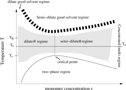
Figure 1: Schematic phase-diagram of a polymer solution as a function of temperature $T$ and monomer concentration $c$, for a finite length $L$. $R_{g}$ decreases with decreasing $T$ so that for good solvents, the monomer concentration at which the dilute regime crosses over to the semi-dilute regime increases. As $T$ is lowered further, there is also a crossover to the “theta regime”, denoted schematically by the shaded region. In the limit $L\rightarrow\infty$, $T_{B}$ and $T_{c}$ both approach $T_{\theta}$, so that the size of the “theta regime” decreases. Furthermore, the monomer concentration at the crossover between the dilute and semi-dilute regimes, as well as that of the critical point, both tend to zero for infinite $L$.

For a finite $L$, there is a “theta solvent regime” of temperatures around $T_{\theta}$, where the polymer behavior most resembles that predicted for theta polymers. The longer the polymer, the sharper the transition between “theta solvent” and “good solvent” regimesdeGe79 ; Rubi03 ; Gras95 . A typical phase-diagram for solutions of polymers of finite length is presented in Fig. 1.

In the low concentration limit, the physical properties of interacting polymers in solution closely resemble those of ideal polymers with the same $R_{g}$. For good solvents, however, important deviations from ideal behavior rapidly set in for increasing concentration, even in the dilute regime, see e.g. ref. Loui02a . On the other hand, the fact that $B_{2}(T,L)\simeq 0$ for $T$ near $T_{\theta}$ suggests that in the theta regime the osmotic pressure $\Pi$ will follow van t’Hoff’s law

$$\beta\Pi\simeq\frac{c}{L}$$ (1)

for a larger concentration range than is found for polymers in good solvent. Nevertheless, as concentration is increased further, the effect of higher order virial coefficients will eventually kick in, leading to deviations from the simple van t’Hoff behavior. Similar differences with ideal-polymer behavior should also be observable for interfacial properties such as the adsorption or surface tension near a hard non-adsorbing wall.

While much theoretical and numerical work on simple models of interacting polymer solutions has been devoted to behavior for athermal conditions, or at $T=T_{\theta}$, less is known about how properties of polymer solutions vary with temperature and concentration in the intermediate regime $(\infty>T\gtrsim T_{\theta})$.

In the present paper we present MC data for the bulk and interfacial properties of dilute and semi-dilute polymer solutions for the same model as used in refGras95 , over a range of temperatures between the athermal (high temperature) limit and $T_{\theta}$. The main objective is a systematic investigation of polymer solution properties over a wide range of concentrations, to determine how equilibrium properties like the osmotic pressure, the adsorption near a wall, the surface tension and the polymer induced depletion potential between two walls vary as thermal conditions change from the good solvent to the theta-solvent regime. In particular we are examining the important problem of how the behavior of polymers in theta-solvent differs from that of ideal (non-interacting) polymers as their concentration increases.

The paper is organized as follows. The polymer lattice model and the computational methodology are introduced in section II. Results for the osmotic equation of state and semi-dilute regimes will be presented and discussed in section III. We shall next turn our attention to monomer density profiles near a non adsorbing wall as well as the polymer-wall surface surface tension as a function of temperature and concentration (section IV). The polymer-induced depletion potential between two walls will be discussed in section VI, and concluding remarks will be made in section VII.

II Model and simulation methodology

II.1 Lattice model of polymer solutions

A familiar coarse-grained representation of linear polymers in a solvent, which captures the essential physical features, is a self-avoiding walk (SAW) lattice polymer, where each lattice site can be occupied by at most one monomer (or polymer segment) to account for excluded volume, and where pairs of non-sequential monomers of nearest-neighbor (n.n.) sites experience an attractive energy $-\beta\epsilon$. The parameter $\epsilon$ accounts for the difference between solvent-solvent, solvent-monomer, and monomer-monomer interactions, and includes both energetic and entropic componentsdeGe79 ; Rubi03 . As the dimensionless ratio $\beta\epsilon=\epsilon/k_{B}T$ increases from zero (corresponding to the athermal solvent limit) to larger values, the quality of the solvent decreases, i.e. effective monomer-monomer attractions become increasingly important, so that the polymer coils tend to shrink until the theta-regime is reached. Upon further cooling at finite concentrations, phase separation sets in at some $T<T_{\theta}$, see e.g. Fig. 1.

In this paper we consider polymer chains made up of $L$ monomers in a simple cubic lattice of $M$ sites (coordination number $z=6$), with periodic boundary conditions. If $N$ polymers live on that lattice, the polymer concentration is $\rho=N/M$, while the monomer concentration is $c=NL/M$. $R_{g}\sim L^{\nu}$, (with $\nu=0.59$ in good solvent, and $\nu=\frac{1}{2}$ in theta solvent) is the radius of gyration of a polymer coil, and the overlap concentration is defined as $1/\rho*=\frac{4}{3}\pi R_{g}^{3}$, where $R_{g}$, which depends on $\beta\epsilon$, will conventionally be chosen to be the radius of gyration in the infinite dilution limit ($\rho\rightarrow 0$) limit. $\rho*$ separates the dilute regime of the polymer solution ($\rho/\rho*<1$) from the semi-dilute regime $(\rho/\rho*>1)$.

In the scaling limit $(L\rightarrow\infty)$, the properties of a polymer solution in the dilute and semi-dilute regimes depend only on $\rho/\rho*$ and $R_{g}$, and are independent of the monomer concentration $c$deGe79 ; Rubi03 . In other words, simulations with different $c$ but the same $\rho/\rho*$ should give equivalent results when length is expressed in units of $R_{g}$. This requires that simulations be carried out with sufficiently long polymers so that the monomer concentration $c\ll 1$. Under good solvent conditions, $R_{g}\approx 0.4L^{0.59}$ for polymers on a simple cubic lattice, so that

$$c*=L\rho*\approx\frac{4}{L^{0.77}},$$ (2)

whereas in theta-solvent, $R_{g}\approx 0.55L^{\frac{1}{2}}$Gras95 , and so

$$c*\approx\frac{1.4}{L^{0.5}}.$$ (3)

Most of the subsequent MC simulations have been carried out for $L=500$ polymers, such that $c*\simeq 0.027$ under good solvent conditions, while $c*\simeq 0.06$ in theta-solvent. In order to ensure that $c<0.25$ in all simulations, the semi-dilute regime which could be explored was hence restricted to $\rho/\rho*<10$ in good solvent, and $\rho/\rho*<4$ in theta-solvent. For higher concentrations, the c-dependence of the results would no longer be negligible, and non-universal effects would become important, depending on the property under consideration. For this reason, much smaller polymers, say $L=100$, could not be used to study the semi-dilute regime.

The previous extensive MC study by Grassberger and HeggerGras95 determined $T_{B}$ as a function of $L$ for a model identical to the one used here. They found that for $L=500$, the Boyle temperature $T_{B}$ gave $\beta\epsilon=0.265$, the value which we shall use throughout the discussion in this paper as a reasonable estimate for the theta-temperature.

II.2 Monte Carlo simulation methodology

We used 4 different types of moves to sample configuration space: The pivot algorithm attempts to rotate part of the polymer around a randomly chosen segment. Translations move the whole polymer through space, and reptations remove a segment at one end of the polymer and attempt to regrow it at the other end. Since translation and pivot rapidly become less efficient for increasing polymer concentration, we also used configurational bias Monte Carlo (CBMC) movesfrenkelbook . These are also very effective at lower temperatures, since the attraction between polymers reduces the accepted number of pivot and translation movesKrak03 .

Simulations were carried out in a box of size $160\times 100\times 100$ for polymers of length $L=500$. For calculations of radii of gyration, and other bulk properties, periodic boundary conditions were used in all directions, whereas for surface properties calculations, hard walls were placed at $0$ and $160$ along the x-axis. The osmotic pressures were calculated using the method of DickmanDick87 . A external repulsive potential $\epsilon_{w}$ that acts between on monomers next to the wall is introduced, and varied such that the parameter $0\leq\lambda=e^{-\epsilon_{w}/k_{B}T}\leq 1$. $\lambda$=0 prevents any particles from being adjacent to the wall, and the varying wall hardness allows the the osmotic pressure $\beta\Pi$ to be calculated from the integral

$$\beta\Pi(\rho)=\int_{0}^{1}\frac{d\lambda}{\lambda}\rho_{w}(\lambda),$$ (4)

where $\rho_{w}(\lambda)$ is the site occupation fraction of monomers right next to the wall. We performed $5$ simulations at different $\lambda$ values, chosen from a standard Gauss-Legendre distribution, to carry out the integral above. By using 2 walls of varying hardness, the statistics are enhanced over using a single wall. Adding repulsive walls increases the bulk density at the center of the simulation cell, an effect which becomes more pronounced for smaller boxes. Thus $N/V$ should not be taken as the bulk density. Instead, we have determined the bulk density by averaging over the region, near the center of the box, where the influence of the two depletion layers have completely decayedStuk02 .

As a first application of the MC code, we have computed the radius of gyration of an isolated polymer for lengths $L=100$ to $L=5000$, and extracted an exponent $R_{g}\sim L^{\nu}$, shown in Fig. 2. For higher temperatures, $\nu=0.588$ within error bars, as expected for the good solvent regime, but for $\beta\epsilon=0.2$ the exponent $\nu$ appears to deviate slightly, and we find $\nu=0.570\pm 0.003$. In the limit $L\rightarrow\infty$, this scaling should be independent of temperature, as long as $T>T_{\theta}$. However, here we observe some rounding, most likely due to finite length crossover effects. The precise temperature at which theta-type scaling behavior of $R_{g}$ sets in is dependent on length. The longer the polymer, the smaller the range of temperatures over which transition from the good-solvent to the theta regime occursGras95 ; Shaf99 . Note also that for a given $L$, the $R_{g}$ for e.g. $\beta\epsilon=0.1$, is smaller than $R_{g}$ for $\beta\epsilon=0$. Nevertheless, the scaling with length, $R_{g}\sim L^{0.59}$, is still the same for those two temperatures, i.e. the polymers are still in the good solvent regime. Thus the effect of lowering the temperature is simply to renormalize the effective step-length.

For $T=T_{B}$, with $T_{B}$ for each length taken from ref. Gras95 , we find $\nu=0.498\pm 0.008$, as expected for the theta regimeLog . As the temperature is lowered further, $\nu$ continues to decrease, and for low enough $T$ the polymer should collapse to a compact globule state where $\nu=\frac{1}{3}$. The beginning of this trend is evident in the plot for $\beta\epsilon=0.285$. The larger error bars reflect the more pronounced finite $L$ effects expected at this temperature. For short polymers the transition from extended to collapsed states occurs over a broad range of temperatures, whereas for longer polymers the collapse transition is sharperGras95 .

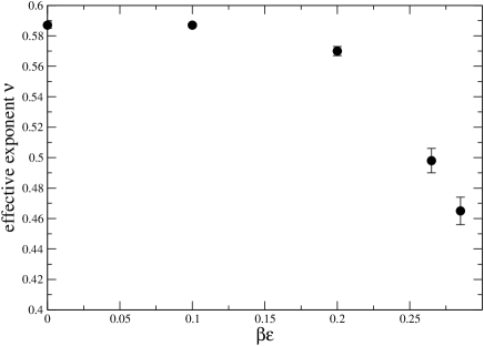
Figure 2: Effective exponents $\nu$, extracted from simulations with different lengths $L$, as a function of $\beta\epsilon$. . Note that the value presented at $\beta\epsilon=0.256$, corresponding to $T_{B}$ for $L=500$, was calculated at slightly different temperatures, corresponding to $T_{B}$, for each polymer length.

$R_{g}$ shrinks (for fixed $L$) as the temperature is lowered, because the excluded volume interactions are partially compensated by attractive interactions between monomers. Similarly in the good solvent regime, $R_{g}$ decreases with density because the excluded volume interactions are screened by overlapping polymer coils. This decrease follows a scaling law $R_{g}\sim\rho^{\frac{1}{8}}$deGe79 ; Rubi03 once the semi-dilute regime is well developedBolh01 . At the theta-temperature, on the other hand, chain statistics are nearly ideal on all length scales and concentrationsRubi03 , so that $R_{g}$ should be independent of concentration. For even lower temperatures, $T_{B}>T>T_{c}$, the screening of attractive interactions now implies that $R_{g}$ should increase with concentration. These trends are indeed observed in our MC simulations, as illustrated in Fig. 3 for $L=500$ polymers.

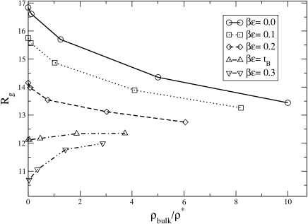
Figure 3: $R_{g}$, calculated for $L=500$ polymers, decreases with concentration for polymers in good solvent, is virtually independent of density for $T=T_{B}$, and increases with concentration when $T<T_{B}$. For each temperature simulations were performed up to a maximum monomer concentration $c\approx 0.25$, so that the total $\rho/\rho*$ range accessible decreases with temperature.

III Equation of state in the dilute and semi-dilute regimes

The thermodynamic property which is most readily extracted from the simulations is the internal energy of polymer solutions, which is simply $U=-\bar{N}_{c}\epsilon$, where $\bar{N}_{c}$ is the average number of nearest-neighbor “contacts” between non-connected monomers. The energy per polymer is $U/N=-\epsilon L\bar{n}_{c}$, where $\bar{n}_{c}$ is the average number of non-connected nearest neighbors around a monomer. Within a simple mean-field picture, $\bar{n}_{c}$ is expected to increase linearly with the polymer concentration. Such linear behavior is indeed observed in Fig. 4 for theta conditions. At higher temperatures, there is a significant downward curvature on $U(\rho)$, while below $T_{B}$, but above $T_{c}$, $U(\rho)$ curves upward.

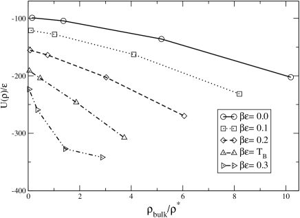
Figure 4: MC data for the reduced internal energy $U(\rho)/\epsilon=-\bar{N}_{c}$ for $L=500$ chains, plotted as a function of polymer concentration $\rho/\rho*$ for 5 different temperatures. Note how the curvature changes with solvent quality.

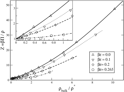
Figure 5: Linear graph of the EOS $Z=\beta\Pi(\rho)/\rho$ as a function of concentration for different temperatures. (Inset) A blowup of the dilute regime highlights the differences between near theta solvents and polymers in good solvent. The former show behavior that mimics that of ideal polymers.

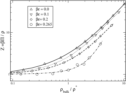
Figure 6: The EOS as a function of concentration for different temperatures, plotted on a double logarithmic scale. In the semi-dilute regime, the EOS is consistent with scaling theory, which predicts $\beta\Pi(\rho)/\rho\sim\rho^{1.3}$ for good solvents and $\beta\Pi(\rho)/\rho\sim\rho^{2}$ for theta solvents.

The osmotic equation of state (EOS) $Z=\Pi(\rho)/(\rho k_{B}T)$ was calculated using Dickman’s methodDick87 described in the previous section. The MC results for $Z$ as a function of $\rho/\rho*$, for various temperatures, are plotted in Figures 5 and 6 on linear and logarithmic scales. As expected, Z increases with $\rho/\rho*$, and decreases with temperaturecrossover . Since the theta-solvent regime is defined by $T\approx T_{B}$, the EOS is expected to be very flat at low polymer concentrations since $T_{B}$ is defined as the temperature at which the second virial coefficient $B_{2}(T,L)$ vanishes in the virial expansiondeGe79 ; Rubi03 :

$$Z=\frac{\beta\Pi}{\rho}=1+B_{2}c+B_{3}c^{2}+{\cal O}(c^{3}).$$ (5)

This is indeed confirmed by the MC results in the dilute regime, as illustrated in the inset of Fig. 6. Up to $\rho/\rho*\simeq 1$, $Z$ hardly rises with $\rho$, i.e. the system behaves like a solution of ideal polymers. At higher concentrations, however, interactions between monomer triplets come into play, so that, according to Eq. (5), $Z$ is expected to increase like $\rho^{2}$, in agreement with a standard scaling argumentdeGe79 ; Rubi03 . The same scaling argument predicts that the EOS of polymers in good solvent scales as $Z\sim\rho^{1/(3\nu-1)}\sim\rho^{1.3}$; the exponent $1.3$ indeed agrees with the slopes of the double logarithmic plots of $Z(\rho)$ shown in Fig. 6, for $\rho/\rho*\gtrsim 1$ and $0\leq\beta\epsilon\leq 0.2$. The slope of the theta-temperature EOS is clearly significantly larger, and compatible with the expected exponent of $2$. However, for the $L=500$ chains used in the present simulations, the accessible semi-dilute regime of concentrations is too small to allow a fully quantitative estimate (c.f. the discussion in section II). Since the EOS of theta-polymers scales with a larger exponent than that of polymers in good solvent, there will eventually be a concentration $\rho/\rho*$ where the EOS of the theta-polymers becomes larger than that of polymers in good solvent. This may, at first sight, seem counter-intuitive, but it should be remembered that for a given size $R_{g}$, theta-polymers are more compact. By extrapolating our simulation data to larger $\rho/\rho*$, we expect the cross-over between theta-polymers and $\beta\epsilon=0$ (SAW) polymers to occur at $\rho/\rho*\gtrsim 35$ which is, in practice, very hard to achieve both in simulations and experimentsextrapolation . On the other hand, if one starts from a solution under good solvent conditions, i.e. “high” temperature, at a given $\rho$, and lowers the temperature, then the EOS will decrease monotonically, because $R_{g}$, and with it the ratio $\rho/\rho*$, decreases with temperature.

IV Monomer density profiles near a non-adsorbing wall

For entropic reasons, polymer solutions will be highly depleted in the vicinity of a non-adsorbing hard wall: since fewer conformations are available to a polymer coil the wall will effectively repel the polymers so that their concentration will drop from the bulk value for distances $z\gtrsim R_{g}$, to a much lower value at contactdeGe79 . The case of polymers in good solvent (in the SAW limit) has been investigated in much detail in ref. Loui02a , where important deviations from ideal polymer behavior were found even in the dilute regime. Here we continue these investigations, but for polymers in solvents of varying quality.

IV.1 Monomer density profiles

Fig 7 compares the present MC results for the reduced monomer density profiles $c(z)/c$ as functions of the distance $z$ from the planar surface in the good solvent $(\beta\epsilon=0$) and theta-solvent ($\beta\epsilon=0.265$) limits for $L=500$ chains, and several bulk concentrations. The differences between the two regimes are very significant. In the dilute regime the density profiles in the theta solvent hardly change, and are remarkably close to that of ideal polymers, while the profiles in good solvent already differ significantly from the latter, and are “pushed” closer toward the hard wall. In the semi-dilute regime, on the other hand, the density profiles of polymers in theta-solvent differ considerably from that of ideal polymers (which is independent of concentration) and instead more closely resemble those of polymers in good solvent, although the depletion “hole” is systematically wider for the former compared to that of the latter. This is illustrated in Fig. 8, where the profiles at three different temperatures are compared at low concentration, and in the semi-dilute regime.

IV.2 Reduced adsorption

The reduced adsorption of polymers near a hard wall is defined asRowl89 :

$$\hat{\Gamma}(\rho)=-\frac{1}{\rho}\frac{\partial(\Omega^{ex}/A)}{\partial\mu}=\int_{0}^{\infty}h(z)dz,$$ (6)

where $\Omega^{ex}/A$ is the surface excess grand potential per unit area $A$, $\mu$ is the chemical potential, and $h(z)=c(z)/c-1$. Because of the depletion hole, $\hat{\Gamma}(\rho)$ is negative, and has the dimension of length. One could replace $c(z)$ by the distribution of the center of mass (CM) of the polymers $\rho_{cm}(z)$. Although the reduced profiles $h_{cm}(z)=\rho_{cm}(z)/\rho-1$ would look different from $h(z)$ (see e.g. Fig.1 of Ref. Loui02a ), the reduced adsorptions would be identical to those calculated from the monomer density profiles, due to the conservation of the number of monomers.

For ideal polymers, the reduced adsorption can be exactly calculated to beAsak54 ; Bolh01 :

$$\hat{\Gamma}^{id}=-2R_{g}/\sqrt{\pi}\approx-1.1284R_{g},$$ (7)

which is independent of concentration. For polymers in good solvent, a renormalization group (RG)Shaf99 calculation predicts that $\hat{\Gamma}(0)\simeq-1.074R_{g}$ for the adsorption in the low-density limitHank99 , which is close to, but slightly less negative than the ideal result (7). As the polymer concentration increases, interactions between monomers of non-ideal polymers cause the depletion layer to shrink, as illustrated by the density profiles shown in Figs. 7 and  8. Thus, in contrast to the case of ideal polymers, where $c(z)/c$, and therefore $\hat{\Gamma}$ is independent of concentration, for interacting polymers the reduced adsorption $\hat{\Gamma}$ should become less negative for increasing polymer concentration. This is indeed what is observed in Fig. 9, where the variation of the reduced adsorption with concentration is shown for several temperatures.

IV.2.1 Adsorption in the dilute regime

In the dilute regime $(\rho/\rho*\lesssim 1)$, there is, once again, a qualitative difference between polymers in theta or good solvent, as highlighted in the inset of Fig. 9. While the curvature of the $\hat{\Gamma}(\rho)$ curves with concentration is negative in good solvent conditions, it is clearly positive under theta-conditions, and changes to negative in the semi-dilute regime. Up to $\rho/\rho*\simeq 1$, the results for $\hat{\Gamma}$ remain close to (but above) the ideal polymer result (7). Note, however, that the relative deviation from ideal polymers is more pronounced than for the osmotic EOS (compare the insets to Figs. 5 and 9), hinting at a stronger effect of three-particle interactions on the adsorption of theta-polymers.

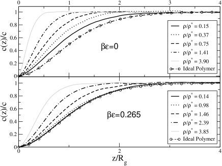
Figure 7: Monomer density profiles $c(z)/c$ for polymers near a hard non-adsorbing wall. The upper panel shows the density profiles for polymers in good solvent, while the lower panel is for polymers at $T=T_{B}$. At these near theta conditions, the density profiles in the dilute regime are nearly indistinguishable from those of ideal polymers, but important deviations emerge in the semi-dilute regime.

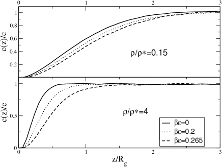
Figure 8: Monomer density profiles as a function of temperature for two densities. The upper panel is for $\rho/\rho*\approx 0.14$, and the lower panel is for $\rho/\rho*\approx 4$, well into the semi-dilute regime. The density profiles at lower temperatures are more extended when plotted in terms of $z/R_{g}$.

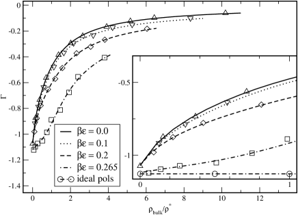
Figure 9: Reduced adsorption $\hat{\Gamma}/R_{g}$ as a function of concentration for several temperatures. (Inset) Blowup of the dilute regime. Note the different curvature at low densities. The values at $\rho/\rho*=0$ are take from theory to be $\hat{\Gamma}/R_{g}=1.074$Hank99 for the first three temperatures, and $\hat{\Gamma}/R_{g}=2/\sqrt{\pi}$ for $T=T_{B}$.

IV.2.2 Adsorption in the semi-dilute regime

In the semi-dilute regime we expect the adsorption to be proportional to the correlation length $\xi/R_{g}\sim(\rho/\rho*)^{-\nu/(3\nu-1)}$deGe79 ; Rubi03 , since this is the only relevant length-scale. Note that the numerical prefactors for different semi-dilute correlation lengths vary with the property one is attempting to describe, see e.g. Huan02 for a very useful discussion of this matter. In our previous paperLoui02a we showed that for polymers in good solvent, the reduced adsorption $\hat{\Gamma}/R_{g}\sim(\rho/\rho*)^{-0.77}$ is consistent with this scaling. Here we present more simulations in the semi-dilute regime to confirm this behavior, finding that $\hat{\Gamma}/R_{g}\sim-0.4(\rho/\rho*)^{-0.77}$ provides a good fit. Scaling theory considerations also predict that $\xi/R_{g}\sim(\rho/\rho*)^{-1}$ for theta solventsdeGe79 ; Rubi03 . However, this behavior cannot be reliably extracted from the current simulations of $\hat{\Gamma}$, which are not performed for a large enough range of $\rho/\rho*$. Furthermore, we expect that for the higher values of $\rho/\rho*$ sampled here, finite $c$ effects may already be coming into play.

V Wall-polymer surface tension

The wall-polymer surface tension, i.e. the free-energy cost of introducing a non-adsorbing hard wall and its associated depletion layer, can be calculated from the adsorption and EOS by use of the Gibbs adsorption equationMao97 :

$$\gamma_{w}(\rho)=\frac{\partial\Omega^{ex}}{\partial A}=-\int_{0}^{\rho}\left(\frac{\partial\Pi(\rho^{\prime})}{\partial\rho^{\prime}}\right)\hat{\Gamma}(\rho^{\prime})d\rho^{\prime}.$$ (8)

By performing one integration by parts w.r.t. density, Eq. (8) can also be expressed as:

$$\gamma_{w}(\rho)=-\Pi(\rho)\hat{\Gamma}(\rho)+\int_{0}^{\rho}\Pi(\rho^{\prime})\left(\frac{\partial\hat{\Gamma}(\rho^{\prime})}{\partial\rho^{\prime}}\right)d\rho^{\prime}.$$ (9)

The first term in this equation has an appealing physical interpretation as the free energy cost per unit area of creating a slab cavity of width $\hat{\Gamma}(\rho)$. For ideal polymers, where $\hat{\Gamma}(\rho)$ is independent of concentration, this term is the only one that contributes, and so $\gamma_{w}^{id}=-\rho\hat{\Gamma}^{id}=-\rho 2/\sqrt{\pi}$. Since the EOS and $\hat{\Gamma}(\rho)$ for interacting polymers in various quality solvents were calculated in the previous sections, we can now, using Eq. (9), determine the surface tension for different solvent qualities. Results are shown in Fig. 10. For good solvent conditions, i.e. $\beta\epsilon=0$, they are, to within simulation errors, in near quantitative agreement with the RG calculations of Maasen, Eisenriegler, and BringerMaas01 . In fact, the larger number of simulation results in the semi-dilute regime, used in the present work, lead to even better agreement than that shown earlier in Ref. Loui02a . We are not aware of theories of comparable quality for the surface tension of theta polymers.

As discussed earlier for the EOS and the adsorption, we again find qualitatively different behavior for the $T=T_{B}$ solution in the dilute regime, as highlighted in the inset of Fig. 10. The surface tension for such theta like solvents resembles that of ideal polymers much more closely than that of polymers in good solvent. As expected from the related behavior of the adsorption, the relative deviation from ideal polymer behavior in the dilute regime is somewhat larger than what was found for the EOS. Note that the curves $\gamma_{w}/\gamma_{id}$ cross at very low $\rho/\rho*$. This follows from the fact that the low concentration limit of the surface tension is given by $\lim_{\rho\rightarrow 0}\beta\gamma_{w}=-\rho\hat{\Gamma}$, and $-\hat{\Gamma}$ is smaller for interacting polymers than for ideal or theta polymers. (See Fig. 9). At slightly higher densities, the curves cross because $\gamma_{w}$ increases more rapidly with concentration for good solvents than for theta solvents.

In the semi-dilute regime, where $\hat{\Gamma}\sim\xi\sim\rho^{-\nu/(3\nu-1)}$ and $\Pi(\rho)\sim\rho^{3\nu/(3\nu-1)}$, Eq. (8) simplifiesLoui02a to

$$\gamma_{w}^{sd}(\rho)\approx\frac{3}{2}\Pi\hat{\Gamma}\sim\rho^{2\nu/(3\nu-1)}.$$ (10)

This implies $\gamma_{w}^{sd}\sim\rho^{1.539}$ semi-dilute scaling for polymers in good solvent, and $\gamma_{w}^{sd}\sim\rho^{2}$ behavior for theta solvents, which is consistent with the results in Fig. 10. Furthermore, this scaling suggests that for large enough $\rho/\rho*$, the surface tension curve for theta polymers will eventually cross that of polymers in good solvent. Indeed, Fig. 10 already appears to suggest this behavior, although some care must be taken in extracting the $\rho/\rho*$ at which crossover occurs, due to the the possibility of finite $c$ effects for theta polymersextrapolation . With these caveats in mind, our results suggest that the surface tension for theta polymers would be greater than that of interacting polymers when $\rho/\rho*\geq 10$, which is considerably lower than the predicted crossing for the EOS, and within reach of experiment and simulations. On the other hand, just as in the case of the EOS, if one were to lower the temperature of an experimental polymer solution at a given $\rho$, this would lead to a lower $\rho/\rho*$, so that a monotonic behavior of $\gamma_{w}$ with temperature is expected when following this route.

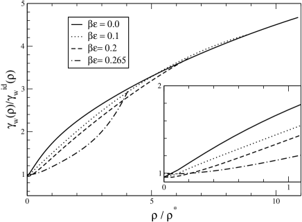
Figure 10: Wall-polymer surface tension divided by the ideal surface tension for various solvent qualities, plotted as a function of concentration $\rho/\rho*$. (Inset) A blowup of the dilute regime highlights the differences between $\gamma_{w}/\gamma_{w}^{id}$ for good and theta solvents.

VI Depletion potentials between two walls

The depletion potential between two walls or plates induced by a polymer solution is defined as the difference in free energy between the cases where the plates are at a distance $z$, or infinitely far apart. The polymer solution between the plates is taken to be in equilibrium with a much larger reservoir of pure polymer solution at the same chemical potential. At infinite distance, the free energy cost of having two plates is simply twice the cost of making a depletion layer, while at contact, these two depletion layers are destroyed. Thus, when $z=0$, the free energy per unit area of plate is given by

$$W(0)=-2\gamma_{w}(\rho).$$ (11)

For small $z$ virtually no polymer is expected to penetrate between the plates, which are hence pressed together by the osmotic pressure $\Pi(\rho)$, leading to a linear increase of $W(z)$ with $z$. As discussed in ref Loui02b , the simplest approximation for the depletion potential is to continue this linear form for larger $z$:

$$W(z)= W(0)+\Pi(\rho)z; \,\,\,\,z\leq D_{w}(\rho)$$

$$W(z)= \,\,\,0\,\,\,\,\,\,\,\,\,\,\,\,\,\,\,\,\,\,\,\,\,\,\,\,\,\,\,\,\,\,; \,\,\,\,z>D_{w}(\rho)$$ (12)

where the range is given by

$$D_{w}(\rho)=-\frac{W(0)}{\Pi(\rho)}=\frac{2\gamma_{w}(\rho)}{\Pi(\rho)}.$$ (13)

We note that this approximation is similar to that adopted by Joanny, Leibler, and de Gennes who, in their pioneering paperJoan79 , approximated the force between two plates as constant for $x\leq\pi\xi(\rho)$ and zero for $x>\pi\xi(\rho)$. This also results in a linear depletion potential.

In ref Loui02b , we showed that this simple theory is virtually quantitative for polymers in good solventTuin03a . Furthermore, it is well known to be quite accurate for ideal polymers as wellBolh01 . Although one could easily generalize the theory to include the small curvature seen for ideal polymers close to $z=D_{w}$Asak54 , we ignore these small corrections in the interests of simplicity. Since this theory is accurate for polymers in good solvent as well as for ideal polymers, we postulate that the same simple assumptions are valid for other solvent qualities, and use Eq. (VI) to calculate the depletion potentials.

The well-depth $W(0)$ follows from Eq. (11), and is shown in Fig. 11. The behavior mirrors that of Fig. 10 of course. From the inset it is clear that theta polymers most closely resemble ideal polymers in the dilute regime, while important deviations are found in the semi-dilute regime.

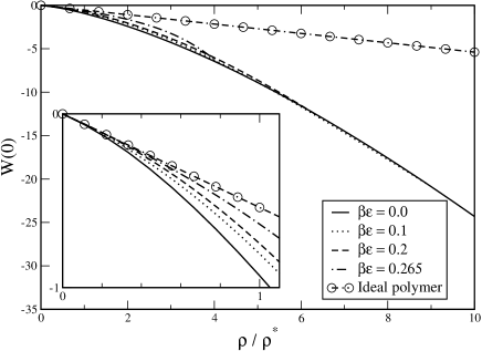
Figure 11: The depletion potential at contact is given by $W(0)=-2\gamma_{w}(\rho)$. (Inset) A blowup of the dilute regime shows that theta polymers most closely resemble the ideal polymers.

In Fig. 12, we plot the range $D_{w}(\rho)$ for a number of different solvent qualities. In the dilute regime, highlighted in the inset, the range for the near theta solvent is fairly close to that of ideal polymers, whereas for polymers in good solvent the range decreases markedly in the dilute regime. In the semi-dilute regime both good and theta solvent regimes show important deviations from ideal polymer behavior. From scaling theory we expect $D_{w}(\rho)\sim\rho^{-0.77}$ and $D_{w}(\rho)\sim\rho^{-1}$ for the polymers in good and theta solvents respectively.

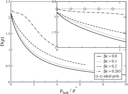
Figure 12: Range of the depletion potential $D_{w}(\rho)$, as given by Eq. (13). In the dilute regime, highlighted in the inset, theta polymers are most similar to ideal polymers, whereas polymers in good solvent already show fairly strong deviations: at $\rho/\rho*=1$ the range has dropped by almost a factor 2 compared to ideal polymers.

The results for $W(0)$ and $D_{w}(\rho)$ can be combined with Eq. (VI) to determine the full depletion potential between two plates. An example, for $\rho/\rho*\approx 1$, is shown in Fig. 13. The depletion potential for theta polymers most closely resembles that of ideal polymers. For lower $\rho/\rho*$ we expect an even closer correspondence.

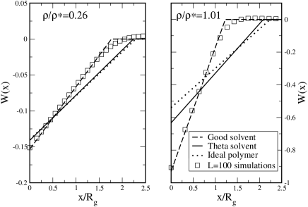
Figure 13: Depletion potentials, calculated via Eq. (VI), for $\rho/\rho*=0.26$ and $\rho/\rho*=1.01$. This simple theory compares well to direct simulations, taken from Loui02b , for good solvents. For theta polymers the depletion potential resembles that of ideal polymers: at $\rho/\rho*=0.26$ they are virtually inistinguishable; at $\rho/\rho*=1.01$ there are slight differences.

In the dilute regime, Figs. 11–13 suggest that the depletion potential between two plates, induced by theta polymers, resembles that of ideal polymers. We have recently shown how to construct depletion potentials between two spheres from that between two platesLoui02b , and found quantitative agreement with direct simulations of $L=500$ SAW polymers between spheres, and also good results for ideal polymers. This suggests that the same procedure should work well for the depletion potential between two spheres induced by theta polymers. Furthermore, since the depletion potentials are the dominant determinant of depletion induced phase separation for $R_{g}/R_{c}\lesssim 1$Meij94 ; Rote04 , we would expect the phase-behavior of theta polymers to closely follow that of ideal polymers, at least for these size ratios. If there are slight deviations, then Fig. 13 suggests that the binodals would shift toward those of polymers in good solvent. Recent experimentsShah03 of colloids mixed with polymers in a near theta solvent indeed show behavior that more closely resembles that of ideal polymers than that of polymers in good solvent.

VII Conclusions

We have performed extensive Monte Carlo simulations to investigate the bulk and interfacial properties of polymers in good solvent, and polymers in the theta regime. For infinite length $L$, there would be a sharp transition between the behavior of polymers in good solvent, and those in a theta solvent. The simulations were carried out for $L=500$, so that continuous cross-over effects are to be expectedGras95 ; Shaf99 . Working out the detailed crossover behavior would require many more simulations at different $L$. However, in practice, most experimentally investigated polymer solutions do not reach the scaling regime either. Moreover, we do observe significant qualitative differences between theta polymers, and polymers with weaker monomer-monomer attraction.

In contrast to polymers in good solvent, solutions of polymers in theta solvent are quite well described by ideal polymer theories throughout the entire dilute regime. This works best for bulk properties like the EOS, and slightly less well for interfacial properties such as the density profiles, adsorptions, and surface tension. However, as predicted by theorydeGe79 ; Rubi03 , in the semi-dilute regime theta polymers also begin to to exhibit important deviations from ideal-polymers. Our simulations show behavior which is consistent with that predicted by scaling theories, but the concentration range we were able to investigate is not wide enough to unambiguously confirm the expected scaling behavior. We also suggest that, for large enough concentrations, the values of various properties, including the EOS, the adsorption, and the surface tension, will be larger for theta polymers than for polymers in good solvent at the same reduced concentration $\rho/\rho*$.

The close agreement between theories for ideal polymers, and our simulations of theta polymers in the dilute regime, suggests that the effective depletion pair potentials, and associated phase behavior, should also resemble those of ideal polymers, at least in the so-called “colloid limit”, where $R_{g}/R_{c}\lesssim 1$.