Numerical Study of Phase Transition in an Exclusion Model with Parallel Dynamics

Abstract

A numerical method based on Matrix Product Formalism is proposed to study the phase transitions and shock formation in the Asymmetric Simple Exclusion Process with open boundaries and parallel dynamics. By working in a canonical ensemble, where the total number of the particles is being fixed, we find that the model has a rather non-trivial phase diagram consisting of three different phases which are separated by second-order phase transition. Shocks may evolve in the system for special values of the reaction parameters.

During the last decade the study of one-dimensional driven lattice gases has been of increasing interest because besides their application in different areas of non-equilibrium physics they show a variety of fascinating properties such as non-equilibrium phase transitions and spontaneous symmetry breaking [1]. They have also let us study the one-dimensional shocks i.e. discontinuities in the density of particles on the lattice over a microscopic region. Depending on the dynamics these models can be divided into two different classes: models with sequential (continuous time evolution) and parallel (discrete time evolution) dynamics. These models can also have open boundaries (where the particles can enter or leave the lattice) or periodic boundary conditions (with conservation of the number of particle).
Different approaches have been used to study the one-dimensional out-of-equilibrium models. Among these approaches the Matrix Product Formalism (MPF) is the one which allows us to study these models under sequential or parallel dynamics with different boundary conditions [2]. According to the MPF the stationary probability distribution function of the system can be written in terms of the matrix element (for the open boundary case) or trace (for the periodic boundary case) of products of non-commuting operators. Several models have been studied using the MPF. In some cases they can be solved exactly; however, in most of the cases exact solutions can only be found in small regions of the reaction parameters space. In a recent work [3] it has been shown that the MPF can be used in order to numerical study of one-dimensional reaction-diffusion models with sequential dynamics and conservation of the number of particles. In the present letter we aim to show that this approach can also be applied to the numerical study of one-dimensional reaction-diffusion models with parallel dynamics and conservation of particles. The Asymmetric Simple Exclusion Process (ASEP) with parallel dynamics will be considered as an example.
In the ASEP with parallel dynamics classical particles move on a one-dimensional lattice of length $L$ (which is assumed to be an even number) with open boundaries. The bulk dynamic is deterministic and consists of two half time steps. In the first half time step particles at even sites move one step to the right provided that their rightmost sites are empty. In this step both the first and the last sites are also updated. From the first (last) site the particles are injected (extracted) with the probability $\alpha$ ($\beta$) provided that the target site is empty (occupied). In the second half time step only the odd sites are updated and the particles at these sites move to the right in the same way. The parallel updating scheme is shown in Fig. 1.

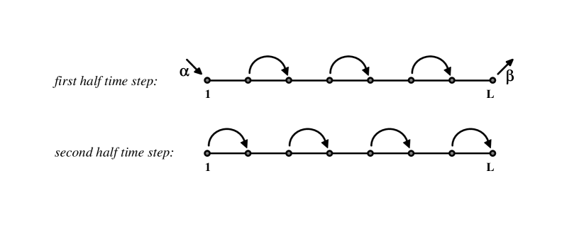
Figure 1: Parallel updating scheme for the ASEP with open boundary.

The ASEP with open boundaries and parallel dynamics has been originally proposed in [4]. Later it was studied using the MPF in [5]. They have both worked in the grand canonical ensemble where the total number of particles in the system is not conserved. The result is that in the large-$L$ limit the model has two different phases: a high-density phase for $\alpha>\beta$ and a low-density phase for $\alpha<\beta$. A first-order phase transition also takes place at the transition point $\alpha=\beta$ where the density profile of particles changes linearly along the lattice. The linear density profile of particles is related to the superposition of shocks in the system. In order to study the shocks one may consider the model on a ring (a lattice with periodic boundary conditions) either in the presence of a slow particle [6, 7, 8], which is sometimes called an impurity, or a slow link [9]. Equivalently one can leave the boundaries open and restrict the total number of particles by working in a canonical ensemble. In the present letter we adopt the latter scenario i.e. we leave the boundaries open; however, the total number of particles on the lattice $M$ (and therefore their density $\rho=\frac{M}{L}$) is restricted to being a constant.
It is shown that the stationary probability distribution function of the ASEP with parallel dynamics can be written as [5]

$$P(\tau_{1},\ldots,\tau_{L})=\frac{1}{Z_{L}}\langle W|\prod_{i=1}^{\frac{L}{2}}[\hat{\mathcal{O}}_{2i-1}\mathcal{O}_{2i}]|V\rangle$$ (1)

in which we have defined

$$\hat{\mathcal{O}}_{i}:=\tau_{i}\hat{D}+(1-\tau_{i})\hat{E}\;,\;\mathcal{O}_{i}:=\tau_{i}D+(1-\tau_{i})E$$ (2)

and $\tau_{i}\in\{0,1\}$ is the occupation number at site $i$. The denominator in (1) is a normalization factor. The matrices ($\hat{D},\hat{E}$) and ($D,E$) are square matrices and besides the vectors $|V\rangle$ and $\langle W|$ are acting in an auxiliary space which might have either a finite or an infinite dimension. They also stand for the presence of particles and holes at odd and even sites respectively and should satisfy the following quadratic algebra

$$\begin{array}[]{l}[E,\hat{E}]=[D,\hat{D}]=0\;,\;E\hat{D}=[\hat{E},D]\;,\;\hat{D}E=0\\ \langle W|\hat{E}(1-\alpha)=\langle W|E\;,\;\langle W|(\alpha\hat{E}+\hat{D})=\langle W|D\\ (1-\beta)D|V\rangle=\hat{D}|V\rangle\;,\;(E+\beta D)|V\rangle=\hat{E}|V\rangle.\end{array}$$ (3)

It has also been shown that (3) has a two-dimensional representation for $\alpha\neq\beta$ [5]

$$\begin{array}[]{l}\hat{D}=\left(\begin{array}[]{cccc}\alpha(1-\beta)&&&0\\ -\alpha\beta&&&0\end{array}\right)\;,\;\hat{E}=\left(\begin{array}[]{cccc}\alpha\beta&&&0\\ \alpha\beta&&&\beta\end{array}\right)\;,\;|V\rangle=\left(\begin{array}[]{c}1-\beta\\ -\beta\end{array}\right)\\ \\ D=\left(\begin{array}[]{cccc}\alpha&&&0\\ -\alpha\beta&&&\alpha\beta\end{array}\right)\;,\;E=\left(\begin{array}[]{cccc}0&&&0\\ \alpha\beta&&&\beta(1-\alpha)\end{array}\right)\;,\;\langle W|=(\alpha,1-\alpha).\end{array}$$ (4)

The normalization factor $Z_{L}$ in (1), which will be called the grand canonical partition function for $\alpha>\beta$ hereafter, can easily be calculated using the fact that $\sum_{\{\mathcal{C}\}}P(\tau_{1},\cdots,\tau_{L})=1$. It is found

$$Z_{L}=\langle W|[(\hat{E}+\hat{D})(E+D)]^{\frac{L}{2}}|V\rangle=(1-\beta)\alpha^{L+1}-(1-\alpha)\beta^{L+1}.$$ (5)

For $\alpha<\beta$ the grand canonical partition function should be defined as $-Z_{L}$. Let us investigate the phase transitions of the model in this case using the classical Yang-Lee theory [10, 11]. One can apply the Yang-Lee theory by finding the roots of the partition function of the system as a function of one of its intensive variables. It can readily be seen that in the thermodynamic limit $L\rightarrow\infty$ the zeros of (5) as a function of $\alpha$ ($\beta$) lie on a circle of radius $\beta$ ($\alpha$). This predicts a first-order phase transition at $\alpha=\beta$. Since the representation of the algebra (3) has a finite dimensional representation, we expect that the density profile of the particles has an exponential behavior in both phases $\alpha<\beta$ and $\alpha>\beta$. This is in agreement with the results obtained in [4, 5] for the phase diagram of the model. As we mentioned above at the phase transition point one finds a linear profile for the density of particles on the lattice. This is related to the superposition of shocks which can be anywhere on the lattice. In what follows we will investigate the phase diagram of the model with fixed number of particles by introducing a canonical partition function as

$$Z_{L,M}=\sum_{\{\tau_{i}=0,1\}}\delta(M-\sum_{i=1}^{L}\tau_{i})\langle W|\prod_{i=1}^{\frac{L}{2}}[\hat{\mathcal{O}}_{2i-1}\mathcal{O}_{2i}]|V\rangle$$ (6)

in which $M$ and $L$ are the number of particles and the length of the system respectively and $\delta(x)$ is the ordinary Kronecker delta function $\delta_{x,0}$. The operators $\hat{\mathcal{O}}_{i}$ and $\mathcal{O}_{i}$ are also defined in (2). It can easily be verified that (6) can be written as

$$Z_{L,M}=\langle W|Coefficient[(\hat{C}C)^{\frac{L}{2}},M]|V\rangle$$ (7)

in which we have defined

$$\begin{array}[]{c}\hat{C}:=\hat{E}+x\hat{D}\\ C:=E+xD\end{array}$$ (8)

where $x$ is a free parameter and $Coefficient[Expr,n]$ gives the coefficient of $x^{n}$ in the expression $Expr$. Note that since $Expr$ is a matrix then $Coefficient[Expr,n]$ gives the coefficient $x^{n}$ of each of its entries. A similar formula has already been introduced in [3] which can be used for the numerical calculation of the canonical partition function of one-dimensional reaction-diffusion models with sequential dynamics. The formula (7) can be useful for numerical studying of phase transitions in out-of-equilibrium systems with parallel dynamics. For the ASEP with parallel dynamics we will calculate (7) as a function of $\alpha$ and $\beta$ for finite values of $L$ and $M$ by using the representation of its quadratic algebra (4).
Now we investigate the density profile of the particles on the lattice which is defined as

$$\rho(i)=\frac{\sum_{\{\mathcal{C}\}}\tau_{i}P(\tau_{i},\cdots,\tau_{L})}{\sum_{\{\mathcal{C}\}}P(\tau_{i},\cdots,\tau_{L})}$$ (9)

where $\mathcal{C}$ is any configuration with a fixed number of particles and $P(\tau_{i},\cdots,\tau_{L})$ is given by (1). The formula (9) can be written in terms of the operators $\hat{D},\hat{E},D,E$ and the vectors $|V\rangle$ and $\langle W|$; however, since the operators for the existence of particles at even and odd sites are not the same we find different expressions for the density of particles at odd and even sites. It can easily be seen that the density of particles at odd and even sites can be written as

$$\begin{array}[]{c}\rho(2i-1)=\frac{1}{Z_{L,M}}\sum_{k=0}^{M-1}\\ \langle W|Coefficient[(\hat{C}C)^{i-1},k]\hat{D}\;Coefficient[C(\hat{C}C)^{\frac{L}{2}-i},M-k-1]|V\rangle\end{array}$$ (10)

and

$$\begin{array}[]{c}\rho(2i)=\frac{1}{Z_{L,M}}\sum_{k=0}^{M-1}\\ \langle W|Coefficient[(\hat{C}C)^{i-1}\hat{C},k]DCoefficient[(\hat{C}C)^{\frac{L}{2}-i},M-k-1]|V\rangle\end{array}$$ (11)

respectively where $i=1,\cdots,\frac{L}{2}$. The formulas (7), (10) and (11) are quite general and can be used for any one-dimensional reaction-diffusion model with open boundaries, parallel dynamics and only one class of particles.
In order to study the phase transitions of the ASEP in canonical ensemble with open boundaries and parallel dynamics, we use the classical Yang-Lee theory by investigating the zeros of (7) in the complex plane of both $\alpha$ and $\beta$ for different values of $L$ and $M$. The particle concentration at odd and even sites will also be calculated from (10) and (11) in each phase. Our numerical calculations show that in the thermodynamic limit ($L\rightarrow\infty,M\rightarrow\infty,\rho=\frac{M}{L}$) the model has two different phase diagrams depending on the density of particles on the lattice $\rho$: For $\rho<\frac{1}{2}$ the phase diagram of the model consists of a low-density and a shock phase which are separated by a second-order phase transition at $\beta_{c}=2\rho$. The reason that the phase transition is of a second-order is that the zeros of (7) as a function of $\beta$, approach the positive real-$\beta$ axis at an angle $\frac{\pi}{4}$ [12]. The canonical partition function (7) as a function of $\alpha$, does not have any real and positive root smaller than one in this case. In the low-density phase $\beta>\beta_{c}$ the density of particles at both even and odd sites changes exponentially along the lattice; however, in the shock phase $\beta<\beta_{c}$ as we move from the first to the last site of the lattice the particle concentration changes abruptly from $\beta$ to $1$ for even sites and from $0$ to $1-\alpha$ for odd sites. For $\rho>\frac{1}{2}$ the phase diagram of the model consists of a high-density and a shock phase which are separated by a second-order phase transition at $\alpha_{c}=2(1-\rho)$. As for the case $\rho<\frac{1}{2}$ the zeros of (7) as a function of $\alpha$, approach the positive real-$\alpha$ axis at an angle $\frac{\pi}{4}$ and therefore the phase transition is of second-order [12]. The canonical partition function (7) as a function of $\beta$ does not have any real and positive root smaller than one in this case. In the high-density phase $\alpha>\alpha_{c}$ the density of particles at both even and odd sites changes exponentially; however, the shock phase in this case takes place at $\alpha<\alpha_{c}$ and the structure of the particles concentrations in quite similar to the shock phase for $\rho<\frac{1}{2}$. The phase diagrams for both $\rho<\frac{1}{2}$ and $\rho>\frac{1}{2}$ cases are shown in Fig. 2.

Figure 2: The phase diagrams of the ASEP in canonical ensemble with parallel dynamics and open boundaries for $\rho<\frac{1}{2}$ (left) and $\rho>\frac{1}{2}$ (right). The small curves show the behaviors of the density profile of particles in each phase.

At $\rho=\frac{1}{2}$ the phase diagram of the model consists of only a shock phase independent of the values of $\alpha$ and $\beta$. For fixed values of the injection and extraction probabilities ($\alpha_{0},\beta_{0}$) the phase diagram of the model consists of three phases which are determined by the density of particles $\rho$. For $0<\rho<\frac{\beta_{0}}{2}$ we are in the low-density phase in which the density of particles changes exponentially along the chain. For $\frac{\beta_{0}}{2}<\rho<1-\frac{\alpha_{0}}{2}$ we are in the shock phase. Finally, for $1-\frac{\alpha_{0}}{2}<\rho<1$ we are in the high-density phase in which the density profile of particles is an exponential function.
The phase diagram of the ASEP in canonical ensemble with parallel dynamics and open boundaries can also be obtained by studying the grand canonical partition function of this model defined as

$$Z_{L}(x)=\langle W|(\hat{C}C)^{\frac{L}{2}}|V\rangle$$ (12)

in which $\hat{C}$ and $C$ are given by (8) and $x$ plays the role of the fugacity of particles. This can easily be calculated and we find

$$\begin{array}[]{c}Z_{L}(x)=(1-\beta)\alpha^{L+1}x^{\frac{L}{2}}(\beta+x(1-\beta))^{\frac{L}{2}}-(1-\alpha)\beta^{L+1}((1-\alpha)+x\alpha)^{\frac{L}{2}}\\ +\alpha(1-\alpha)\beta(1-\beta)(1-x)(x\alpha+\beta)\\ \sum_{i=0}^{\frac{L}{2}-1}x^{\frac{L}{2}-i-1}\alpha^{L-2i-2}\beta^{2i}(\beta+x(1-\beta))^{\frac{L}{2}-i-1}((1-\alpha)+x\alpha)^{i}.\end{array}$$ (13)

Now let us study the total density of particles as a function of the fugacity $x$

$$\rho(x)=\frac{x}{L}\frac{\partial}{\partial x}\log Z_{L}(x).$$ (14)

In Fig. 3 we have plotted $\rho(x)$ as a function of $x$ for $L=15000$, $\alpha=0.8$ and $\beta=0.4$. As can be seen, the density of particles is an increasing function of $x$ up to a critical point $x_{0}$ where a finite discontinuity takes place. Above the critical point $x_{0}$ the density increases very slowly and remains smaller than unity unless $\alpha\rightarrow 0$. Our numerical calculations show that the discontinuity starts from $\rho_{1}=\frac{\beta}{2}$ and ends at $\rho_{2}=1-\frac{\alpha}{2}$ (see Fig. 3). This is quite in agreement with the picture that we got for the phase diagram of this model.

Figure 3: The density of particles $\rho(x)$ as a function of their fugacity $x$ for $L=15000$, $\alpha=0.8$ and $\beta=0.4$. The critical densities are $\rho_{1}=\frac{\beta}{2}=0.2$ and $\rho_{2}=1-\frac{\alpha}{2}=0.6$.

For $x<x_{0}$ and $x>x_{0}$ the density of particles is determined by their fugacity; however, at $x_{0}$ the fugacity does not fix the density. Here is where we have shocks in the system. This phenomenon has already been observed in other models where the Bose-Einstein condensation takes place and the conservation of the number of particles is broken [13].
In this letter we have investigated the phase transitions and shock formation in the ASEP with open boundaries and parallel dynamics in a canonical ensemble where the total number of particles is kept fixed. We have found that the phase diagram of the model depends of the value of the density of particles on the system. The system can be in any of its three accessible phases: the low-density phase, the high-density phase and the shock-phase. In the shock-phase, the shock position is fixed and determined by the number of particles while in the hight-density and the low-density phases the density profile of the particles at both even and odd sites have exponential behaviors. Since the representation of the associated algebra (3) is finite dimensional, we do not expect the density profile of particles on the lattice to have algebraic behavior [14].

References

- [1] G.M. Schütz Phase Transitions and Critical Phenomena vol 19 ed C. Domb and J. Lebowitz (New York: Academic Press 1999)
- [2] B. Derrida, M.R. Evans, V. Hakim and V. Pasquier J. Phys. A: Math. Gen. A 26 1493 (1993)
- [3] F.H. Jafarpour Physics Letters A 322 270 (2003)
- [4] G.M. Schütz Phys. Rev. E 47 4265 (1993)
- [5] H. Hinrichsen J. Phys. A: Math. Gen. A 29 L305 (1996)
- [6] K. Mallick J. Phys. A: Math. Gen. A 29 5375 (1996)
- [7] H-W. Lee, V. Popkov and D. Kim J. Phys. A: Math. Gen. A 30 8497 (1997)
- [8] F.H. Jafarpour J. Phys. A: Math. Gen. A 33 8673(2000)
- [9] H. Hinrichsen and S. Sandow J. Phys. A: Math. Gen. A 30 2745 (1997)
-
[10]
C.N. Yang and T.D. Lee Phys. Rev. 87 404 (1952)
C.N. Yang and T.D. Lee Phys. Rev. 87 410 (1952) -
[11]
S. Grossmann and W. Rosenhauer Z. Phys. 218 437 (1969)
S. Grossmann and V. Lehmann Z. Phys. 218 449 (1969) - [12] R.A. Blythe and M.R. Evans Brazilian Journal of Physics 33 464 (2003)
- [13] F.H. Jafarpour J. Stat. Phys. 113 269 (2003)
- [14] H. Hinrichsen, K. Krebs and I. Peschel J. Phys. A: Math. Gen. A 29 2643 (1996)