Fractional flux periodicity in tori made of square lattice

Abstract

This paper describes a study on fractional flux periodicity of the ground state in planar systems made from a square lattice whose boundary is compacted into a torus. It is pointed out that, in the long length and large diameter limit of a torus, the ground-state energy and persistent currents show a fractional period of the fundamental unit of magnetic flux depending on the twist around the torus axis. We discuss the possible relationship between the twist and genus of a torus, and comment on fractional flux periodicity in a cylinder.

1 Introduction

The fact that a single electron wave function has a fundamental unit of magnetic flux $\Phi_{0}=2\pi/e$  is known to be an essential consequence of quantum mechanics and is manifest in the Aharonov-Bohm effect [1]. The solid state properties of materials are governed by many electrons, and each constituent has the $\Phi_{0}$ periodicity. However, the fundamental flux period of a material is not always $\Phi_{0}$. For instance, superconductors exhibit a period of $\Phi_{0}/2$, which can be understood by charge doubling due to the Cooper pair formation. This must be a trivial fact if one suppose that a fundamental particle (or quasiparticle) has a $-2e$ charge due to attractive interaction, and that the fundamental flux period of a material is equal to that of the quasiparticle in the system ($2\pi/2e$).

In Fig. 1, we depict schematic diagrams of typical experimental settings for the Aharonov-Bohm effect. Consider an electron going over and under a very long impenetrable cylinder, denoted as a black circle in Fig. 1(a). In the cylinder there is a magnetic field parallel to the cylinder axis, taken as normal to the plane of the figure. The probability of finding this electron in the interference region depends on the magnetic field $\Phi$ and the interference pattern having period $\Phi_{0}$. When an electron is placed in a ring pierced by a magnetic flux $\Phi$ as shown in Fig. 1(b), a current $I$ defined by differentiating the ground state energy with respect to the magnetic flux, appears and is expected to have the flux periodicity $\Phi_{0}$.

\psfrag{a}{(a)}\psfrag{b}{(b)}\psfrag{p}{$\Phi$}\psfrag{I}{$I$}\includegraphics[scale={0.6}]{AB.eps}

Figure 1: Schematic diagram of (a) an Aharonov-Bohm experiment and (b) Aharonov-Bohm ring. In (a), electrons are emitted from the source region, denoted by the empty circle, and produce the interference pattern. In (b), one-dimensional ring is pierced by a magnetic field and exhibits a persistent current.

Actual mesoscopic rings contain many electrons, and non vanishing currents, known as persistent currents [2, 3, 4], are also expected. Although the ground state in mesoscopic rings consists of many electrons, because each electron has the flux periodicity $\Phi_{0}$ one might think the flux periodicity of the systems is the same as the flux periodicity of the constituent electron. In this paper, we present an example in which the fundamental flux period of the ground-state does not coincide with the flux periodicity of the constituent particle. We will show that a fractional flux periodicity ($\Phi_{0}/2,\Phi_{0}/3,\cdots$) can be realized in a certain limit of planar systems made from a square lattice whose geometry is a torus . To analyze the flux periodicity of the systems, we consider the ground state energy and persistent currents. These are considered suitable for examining the flux periodicity of the ground state since they are regarded as the Aharonov-Bohm effect in solid state systems [4]. In the previous paper [5], we showed a typical example of a fractional periodicity in the Aharonov-Bohm effect. Here, we extend the theory in general cases and give detailed derivation of the results.

This paper is organized as follows. In Section 2, we obtain an explicit formula for the ground state energy and plot it for different lattice structures, showing flux periodicity numerically. In Section 3, we examine the persistent currents and prove fractional flux periodicity in the long length and large diameter limit of a torus noting that the characteristic features of the ground state energy can be understood in terms of the twist-induced gauge field. In Section 4, we give a discussion and summary of our results. In Appendix A, we prove a formula used in the text and estimate a correction to a fractional periodicity. Throughout this paper we ignore electron spin and the effect of finite temperature, and consider a half-filling system.

2 Ground state energy

The lattice structure of a torus is specified by two vectors: the chiral , given by $C_{h}=NT_{x}+MT_{y}$, and the translational, given by $T_{w}=PT_{x}+QT_{y}$, where $N,M,P$ and $Q$ are integers and $T_{a}$ ($a=x,y$) is the unit vector of the square lattice in the direction of $x$ and $y$ where we define $x$ and $y$ in the two dimensional map (see Fig. 3(b)). Here, $C_{h}$ $(T_{w})$ characterizes the lattice structure around (along) the tube axis. We rewrite $T_{a}$ in terms of the chiral and translational vectors for a later convenience as

$$\begin{pmatrix}T_{x}\cr T_{y}\end{pmatrix}=\frac{1}{N_{s}}\begin{pmatrix}Q&-M\cr-P&N\end{pmatrix}\begin{pmatrix}C_{h}\cr T_{w}\end{pmatrix},$$ (1)

where we define $N_{s}\equiv NQ-MP$, and $|N_{s}|$ corresponds to the number of square lattices on the surface of the torus given by $C_{h}\times T_{w}=N_{s}(T_{x}\times T_{y})$. In this paper, we take the $x$ axis in the direction of $C_{h}$ ($M=0$), and denote $P=\delta N$ to describe the twist around the tube axis. Then, $C_{h}\cdot T_{w}=\delta NNa^{2}$ where $a(=|T_{x}|=|T_{y}|)$ is the lattice constant. We depict an example of twisted torus in Fig. 2, in which all sites are connected by a line consisting nearest-neighbor bond.

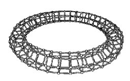
Figure 2: Lattice structure of a twisted torus. The lattice configuration is given by $N=6$, $Q=40$ and $\delta N=1$.

Fig. 3(a) shows an illustration of the twisted torus. A torus can be unrolled to a parallelogram sheet as shown in Fig. 3(b). In the figure, the two lines extending upward from ‘u’ and downward from ‘d’ and having the same ‘$x$’ at the junction are not joined for a twisted torus, as shown in the inset of Fig. 3(a). There are $\delta N$ square lattices between the two lines.

\psfrag{a}{(a)}\psfrag{b}{(b)}\psfrag{C_h}{$C_{h}=NT_{x}$}\psfrag{T_w}{$T_{w}=\delta NT_{x}+QT_{y}$}\psfrag{k}{$\delta N$}\psfrag{x}{$x$}\psfrag{y}{$y$}\psfrag{u}{u}\psfrag{d}{d}\psfrag{T}{$\delta N$}\includegraphics[scale={0.4}]{torus.eps}

Figure 3: Schematic diagram of (a) a twisted torus (upper) and the extension around a cross section (lower), and (b) its net diagram. It is convenient to consider a parallelogram sheet of square lattice as the net diagram of a twisted torus, where the chiral and translational vectors become the vectors at the sides of the parallelogram. The lattice configuration is given by $N=14$, $Q=16$ and $\delta N=-3$.

We consider the quantum mechanical behavior of conducting electrons on a square lattice using the nearest-neighbor tight-binding Hamiltonian:

$${\cal H}=-t\sum_{i}\sum_{a=x,y}a_{i+a}^{\dagger}e^{-ieA^{\rm ex}\cdot T_{a}}a_{i}+h.c.,$$ (2)

where $t$ is the hopping integral, $A^{\rm ex}$ is a constant external gauge field, and $a_{i}$ and $a_{i}^{\dagger}$ are canonical annihilation-creation operators of the electrons at site $i$ that satisfy the anti-commutation relation $\{a_{i},a_{j}^{\dagger}\}=\delta_{ij}$. We diagonalize ${\cal H}$ in terms of the Bloch basis parametrized by wave vector $k$ and obtain ${\cal H}=\sum_{k}E(k-eA^{\rm ex})a_{k}^{\dagger}a_{k}$, where $a_{k}\equiv\frac{1}{\sqrt{|N_{s}|}}\sum_{i}e^{ik\cdot r_{i}}a_{i}$ is the annihilation operator of the Bloch orbital. The energy eigenvalue of the Hamiltonian $E(k-eA^{\rm ex})$ is given by,

$$E(k-eA^{\rm ex})=-2t\Re\left(\sum_{a=x,y}e^{i(k-eA^{\rm ex})\cdot T_{a}}\right).$$ (3)

The Bloch wave vector satisfies the periodic boundary condition for $C_{h}$ and $T_{w}$ through which the geometrical (or topological) information of a torus, such as the twist, is entered into the energy eigenvalue. We decompose wave vector $k$ as $\mu_{1}k_{1}+\mu_{2}k_{2}$, where $k_{1}$ and $k_{2}$ are defined by

$$C_{h}\cdot k_{1}=2\pi,\ C_{h}\cdot k_{2}=0,\ T_{w}\cdot k_{1}=0\ \text{and}\ T_{w}\cdot k_{2}=2\pi.$$ (4)

Here, $k_{1}$ and $k_{2}$ can be rewritten in terms of the reciprocal lattice vectors $K_{x}$ and $K_{y}$ as

$$k_{1}=\frac{1}{N_{s}}(QK_{x}-\delta NK_{y}),\ \ \ k_{2}=\frac{1}{N_{s}}(NK_{y}),$$ (5)

where the reciprocal lattice vectors are defined by $K_{a}\cdot T_{b}=2\pi\delta_{ab}$ with $a,b=x,y$. Components $\mu_{1}$ and $\mu_{2}$ are quantum numbers (integers) and define the Brillouin zone as

$$\left[-\frac{N}{2}\right]+1\leq\mu_{1}\leq\left[\frac{N}{2}\right],\ \ \ \left[-\frac{Q}{2}\right]+1\leq\mu_{2}\leq\left[\frac{Q}{2}\right],$$ (6)

where $[n]$ indicates the maximum integer smaller than $n$.

We point out that the wave vector shifts according to the twist of a torus. For example, in the absence of twist ($\delta N=0$), $k_{1}$ and $k_{2}$ are proportional to $K_{x}$ and $K_{y}$, respectively and perpendicular to each other; otherwise, they are not. The shift of the wave vector plays an important role when we consider the ground state configuration, which we discuss below. Here we rewrite Eq.(3) by means of Eqs.(1) (with $M=0$ and $P=\delta N$) and (4) as

$$E(k-eA^{\rm ex})=-2t\ \left\{\cos\left(\frac{2\pi\mu_{1}}{N}\right)+\cos\left(\frac{2\pi(\mu_{2}-\frac{\delta N}{N}\mu_{1})-eA^{\rm ex}\cdot T_{w}}{Q}\right)\right\},$$ (7)

where we assume $A^{\rm ex}\cdot C_{h}=0$, and $A^{\rm ex}\cdot T_{w}$ corresponds to the Aharonov-Bohm flux penetrating the center of the torus.

\psfrag{x}{$K_{x}$}\psfrag{y}{$K_{y}$}\psfrag{t1}{$T_{x}$}\psfrag{t2}{$T_{y}$}\psfrag{a}{$\frac{\pi}{a}$}\psfrag{k+}{$k^{+}$}\psfrag{k-}{$k^{-}$}\psfrag{s+}{$k_{+}$}\psfrag{s-}{$k_{-}$}\psfrag{s}{(a)}\psfrag{l}{(b)}\psfrag{X}{$\frac{K_{x}}{N}$}\psfrag{Y}{$\frac{K_{y}}{Q}$}\psfrag{m}{$\mu_{1}>0$}\psfrag{n}{$\mu_{1}<0$}\psfrag{A}{$-|\mu_{1}|\frac{\delta N}{N}$}\psfrag{B}{$+|\mu_{1}|\frac{\delta N}{N}$}\includegraphics[scale={0.5}]{F-surface.eps}

Figure 4: Brillouin zone and Fermi lines in momentum space (a), and schematic diagram of the wave vector shifting due to the twist around the axis (b). There are two factors we should take into account to define the ground state. The first factor is the effect of the twist. Compared with the ground-state configuration in an untwisted torus, Eq.(5) indicates that the location of the energy eigenstates shifts depending on twist $\delta N$ and on the electron motion around the axis ($\mu_{1}$). This shift is illustrated in (b), where we denote the Bloch states as circles and depict several states of positive $\mu_{1}$, negative $\mu_{1}$ and $\mu_{1}=0$. In the absence of twist, all states are located at mesh line crossings. When twist is present, the states shift depending on their $\mu_{1}$ and $\delta N/N$. The second factor is the external gauge field. The external gauge field can shift the wave vector, however, the shift is independent of electron motion contrary to the case where twist is present.

The ground state is defined as the state for which all electronic states below (above) the Fermi surface are occupied (empty). We consider a half-filling system and set the Fermi energy $E_{\rm F}=0$. We define the Fermi line in the two dimensional Brillouin zone, within which all states are occupied, as the solution of $E(k)=0$, forming a square as shown in Fig. 4(a). The side of the square (or Fermi line) is denoted by $k^{\pm}$ and $k_{\pm}$. Each energy eigenstate is labeled by $\mu_{1}$ and $\mu_{2}$ and thus we can specify the occupied states by $\mu_{1}$ and $\mu_{2}$ explicitly. In fact the region inside the Fermi line is defined as

$$-\pi\leq\frac{2\pi\mu_{1}}{N}+\frac{2\pi(\mu_{2}-\frac{\delta N}{N}\mu_{1})-eA^{\rm ex}\cdot T_{w}}{Q}\leq\pi,$$ (8)

$$-\pi\leq\frac{2\pi\mu_{1}}{N}-\frac{2\pi(\mu_{2}-\frac{\delta N}{N}\mu_{1})-eA^{\rm ex}\cdot T_{w}}{Q}\leq\pi,$$ (9)

where we note that the Fermi lines satisfy $k^{\pm}\cdot(T_{x}+T_{y})=\pm\pi$ and $k_{\pm}\cdot(T_{x}-T_{y})=\pm\pi$, and Eqs.(8) and (9) can be rewritten as

$$k^{-}\cdot(T_{x}+T_{y})\leq(k-eA^{\rm ex})\cdot(T_{x}+T_{y})\leq k^{+}\cdot(T_{x}+T_{y}),$$ (10)

$$k_{-}\cdot(T_{x}-T_{y})\leq(k-eA^{\rm ex})\cdot(T_{x}-T_{y})\leq k_{+}\cdot(T_{x}-T_{y}).$$ (11)

For a fixed value of $\mu_{1}$, we obtain the following region of $\mu_{2}$, in which all states are occupied by electrons:

$$\left[-Q\left(\frac{1}{2}-\frac{\mu_{1}}{N}\right)+\frac{\delta N}{N}\mu_{1}+N_{\Phi}\right]+1\leq\mu_{2}\leq\left[Q\left(\frac{1}{2}-\frac{\mu_{1}}{N}\right)+\frac{\delta N}{N}\mu_{1}+N_{\Phi}\right],$$ (12)

for $\mu_{1}\geq 0$, and

$$\left[-Q\left(\frac{1}{2}+\frac{\mu_{1}}{N}\right)+\frac{\delta N}{N}\mu_{1}+N_{\Phi}\right]+1\leq\mu_{2}\leq\left[Q\left(\frac{1}{2}+\frac{\mu_{1}}{N}\right)+\frac{\delta N}{N}\mu_{1}+N_{\Phi}\right],$$ (13)

for $\mu_{1}\leq 0$, respectively. Here, we set $A^{\rm ex}\cdot T_{w}=\Phi$ and define the number of Aharonov-Bohm flux $N_{\Phi}\equiv\Phi/\Phi_{0}$. The ground-state energy is therefore

$$E_{0}(\Phi)=\sum_{\mu_{1}=\left[-\frac{N}{2}\right]+1}^{\left[\frac{N}{2}\right]}\sum_{\mu_{2}=\left[-Q\left(\frac{1}{2}-\frac{|\mu_{1}|}{N}\right)+\frac{\delta N}{N}\mu_{1}+N_{\Phi}\right]+1}^{\left[Q\left(\frac{1}{2}-\frac{|\mu_{1}|}{N}\right)+\frac{\delta N}{N}\mu_{1}+N_{\Phi}\right]}E(k-eA^{\rm ex}).$$ (14)

This is the explicit mathematical expression for the ground state energy of a twisted torus.

\psfrag{x}{$N_{\Phi}$}\psfrag{y}{Ground state energy $E_{0}(\Phi)/4t$}\includegraphics[scale={0.8}]{g-ene-dN.eps}

Figure 5: Ground state energy as a function of flux. We fix $N=80$ and $Q=160$, then plot for $\delta N=1,20,40$ to examine the dependence of the ground-state energy on twist. The observed flux periodicity seems to be $\Phi_{0}/2$ for $\delta N=1$ (solid line) and $\delta N=40$ (dashed line) and $\Phi_{0}/4$ for $\delta N=20$ (dotted line). For the untwisted torus ($N=40$, $Q=160$ and $\delta N=0$), refer to Fig. 7(a).

Here, we plot $E_{0}(\Phi)/4t$ for different $N$, $\delta N$ and $Q$ as a function of $N_{\Phi}$, and observe the characteristics of the results. Fig. 5 shows the dependence of the ground state energy on $\delta N$, where we fix $N=80$ and $Q=160$ and vary the twist as $\delta N=1,20,40$. The flux periodicity seems to be $\Phi_{0}/2$ for $\delta N=1$ (solid line) and $\delta N=40$ (dashed line), and $\Phi_{0}/4$ for $\delta N=20$ (dotted line). It appears that flux periodicity of the dashed and dotted lines corresponds to the lattice structure of $\delta N/N$. We note that $\Phi_{0}/2$ periodicity of solid line ($\delta N=1$: odd number) is accurate in our numerical data (10-figure numbers) and that of dashed line ($\delta N=40$: even number) is approximate one. In addition to observing flux periodicity, we see that the solid line is smooth (no cusp) at $N_{\Phi}=0$ for example, when compared with the other two lines.

Next we examine the dependence of the ground state energy on the diameter of the tube $N$. Figs. 6(a), 6(b) , 6(c) and 6(d) show the ground state energy with fixed $Q=160$ and $\delta N=20$ while varying $N=40,80,81,160$. Observing the flux periodicity of the samples, they appear to be periodic in Figs. 6(a) and  6(b) with a period of $\Phi_{0}/2$ in Fig. 6(a) and $\Phi_{0}/4$ in Fig. 6(b). They are not periodic, however, due to a small modulation in the ground state energy. This is manifest in Figs. 6(c) and  6(d). This modulation can be thought of as a finite size correction which will be discussed in Section 3.

\psfrag{x}{$N_{\Phi}$}\psfrag{y}{$(E_{0}(\Phi)-E_{0}(0))/4t$}\includegraphics[scale={0.5}]{g-ene-N40.eps}

(a) Ground state energy for $N=40$, $Q=160$ and $\delta N=20$. We plot $(E_{0}(\Phi)-E_{0}(0))/4t$ where $E_{0}(0)/4t=-1296.892$.

\psfrag{x}{$N_{\Phi}$}\psfrag{y}{$(E_{0}(\Phi)-E_{0}(0))/4t$}\includegraphics[scale={0.5}]{g-ene-N80.eps}

(b) Ground state energy for $N=80$, $Q=160$ and $\delta N=20$. We plot $(E_{0}(\Phi)-E_{0}(0))/4t$ where $E_{0}(0)/4t=-2593.812$.

\psfrag{x}{$N_{\Phi}$}\psfrag{y}{$(E_{0}(\Phi)-E_{0}(0))/4t$}\includegraphics[scale={0.5}]{g-ene-N81.eps}

(c) Ground state energy for $N=81$, $Q=160$ and $\delta N=20$. We plot $(E_{0}(\Phi)-E_{0}(0))/4t$ where $E_{0}(0)/4t=-2626.2443$.

\psfrag{x}{$N_{\Phi}$}\psfrag{y}{$(E_{0}(\Phi)-E_{0}(0))/4t$}\includegraphics[scale={0.5}]{g-ene-N160.eps}

(d) Ground state energy for $N=160$, $Q=160$ and $\delta N=20$. We plot $(E_{0}(\Phi)-E_{0}(0))/4t$ where $E_{0}(0)/4t=-5187.640$.

Figure 6: Dependence of the ground state energy on the diameter of the tube $N$.

Finally, we observe the dependence of the ground state energy on $Q$ shown in Figs. 7(a), 7(b), 7(c) and 7(d). Here, we note that all previous examples except Fig. 6(c) have had the common feature of $Q$ as a multiple of $N$. Fig. 7(a) shows the standard flux periodicity $\Phi_{0}$. In Fig. 7(c), however, we have an approximate periodicity of $\Phi_{0}/2$ even in the absence of twist. We note that $\Phi_{0}/2$ periodicity in Fig. 7(d) ($Q=181$: odd number) is accurate in our numerical data.

\psfrag{x}{$N_{\Phi}$}\psfrag{y}{$(E_{0}(\Phi)-E_{0}(0))/4t$}\includegraphics[scale={0.5}]{g-ene-Q160.eps}

(a) Ground state energy for $N=40$, $Q=160$ and $\delta N=0$. We plot $(E_{0}(\Phi)-E_{0}(0))/4t$ where $E_{0}(0)/4t=-1296.83$.

\psfrag{x}{$N_{\Phi}$}\psfrag{y}{$(E_{0}(\Phi)-E_{0}(0))/4t$}\includegraphics[scale={0.5}]{g-ene-Q170.eps}

(b) Ground state energy for $N=40$, $Q=170$ and $\delta N=0$. We plot $(E_{0}(\Phi)-E_{0}(0))/4t$ where $E_{0}(0)/4t=-1377.965$.

\psfrag{x}{$N_{\Phi}$}\psfrag{y}{$(E_{0}(\Phi)-E_{0}(0))/4t$}\includegraphics[scale={0.5}]{g-ene-Q180.eps}

(c) Ground state energy for $N=40$, $Q=180$ and $\delta N=0$. We plot $(E_{0}(\Phi)-E_{0}(0))/4t$ where $E_{0}(0)/4t=-1459.008$.

\psfrag{x}{$N_{\Phi}$}\psfrag{y}{$(E_{0}(\Phi)-E_{0}(0))/4t$}\includegraphics[scale={0.5}]{g-ene-Q181.eps}

(d) Ground state energy for $N=40$, $Q=181$ and $\delta N=0$. We plot $(E_{0}(\Phi)-E_{0}(0))/4t$ where $E_{0}(0)/4t=-1467.135$.

Figure 7: Dependence of the ground state energy on the diameter of the torus $Q$.

It is important to mention that flux periodicity and the amplitude of the oscillation of $E_{0}(\Phi)$ depends much on $N$, $Q$ and $\delta N$. We will discuss the dependence of the flux periodicity and amplitude on them in the next section.

3 Persistent currents and interpretation of the numerical results

In the previous section, we presented a formula for the ground state energy. By plotting the energy for different values of $N,\delta N$ and $Q$, we found that some tori exhibit an approximate fractional flux periodicity. In this section, we will present an analytical results that demonstrate and prove fractional flux periodicity in the long length ($Q\gg 1$) and large diameter ($N\gg 1$) limit for a twisted torus in terms of the persistent currents. By so doing, we clarify the relationship between the lattice structure and flux periodicity.

Persistent current is defined by differentiating the ground state energy with respect to the magnetic flux $\Phi$ [4]:

$$I_{\rm pc}(\Phi)=-\frac{\partial E_{0}(\Phi)}{\partial\Phi}.$$ (15)

Because $E_{0}(\Phi)$ consists of many energy dispersion relations as specified by $\mu_{1}$ (hereafter referred to as $\mu_{1}$-th energy band), we can write

$$E_{0}(\Phi)=\sum_{\mu_{1}=\left[-\frac{N}{2}\right]+1}^{\left[\frac{N}{2}\right]}E(\mu_{1},\Phi)$$ (16)

where $E(\mu_{1},\Phi)$ is the ground state energy of $\mu_{1}$-th energy band and is the sum of the energy at $\mu_{2}$-th $k$ points which satisfy Eqs.(12) and (13):

$$E(\mu_{1},\Phi)\equiv\sum_{\mu_{2}=\left[-Q\left(\frac{1}{2}-\frac{|\mu_{1}|}{N}\right)+\frac{\delta N}{N}\mu_{1}+N_{\Phi}\right]+1}^{\left[Q\left(\frac{1}{2}-\frac{|\mu_{1}|}{N}\right)+\frac{\delta N}{N}\mu_{1}+N_{\Phi}\right]}E(\mu_{1}k_{1}+\mu_{2}k_{2}-eA^{\rm ex}).$$ (17)

Hence, the persistent current can also be decomposed into the current of each energy band as

$$I_{\rm pc}(\Phi)=\sum_{\mu_{1}=\left[-\frac{N}{2}\right]+1}^{\left[\frac{N}{2}\right]}I(\mu_{1},\Phi),\ \text{ where $I(\mu_{1},\Phi)\equiv-\frac{\partial E(\mu_{1},\Phi)}{\partial\Phi}$}.$$ (18)

To calculate the persistent currents in long systems with $|T_{w}|\gg a$ (or $Q\gg 1$), it is not necessary to sum over the energy eigenvalue of the valence electrons but just calculate the Fermi velocity of the energy band. Because, when we vary the magnetic field, the change of the ground state energy is almost determined by the change of the energy eigenvalue of electrons near the Fermi level and that of the energy eigenvalues deep in energy bands cancel to one another. Using Fermi velocity, the amplitude of $I(\mu_{1},\Phi)$ (the persistent current for the $\mu_{1}$-th energy band) is well approximated by [4]

$$I(\mu_{1})=\frac{ev_{F}(\mu_{1})}{|T_{w}|},$$ (19)

where $|T_{w}|$ is the system length and $v_{F}(\mu_{1})$ denotes the Fermi velocity of the $\mu_{1}$-th energy band. The proof of this approximation is given in Appendix A. By fixing $\mu_{1}$ and expanding Eq.(7) on $\mu_{2}$ around the Fermi level, we obtain the energy dispersion relation of the $\mu_{1}$-th energy band as

$${\cal H}_{\mu_{1}}=v_{F}(\mu_{1})p_{2}+{\cal O}(p_{2}^{2}).$$ (20)

where $p_{2}(\equiv\mu_{2}k_{2})$ denotes the momentum along the axis. Here, we neglect an external gauge field. Notice that Eq.(20) represents the case for $\mu_{2}>0$, and for $\mu_{2}<0$, the energy dispersion relation is given by $-{\cal H}_{\mu_{1}}$ up to ${\cal O}(p_{2})$. The coefficient of $p_{2}$ is the Fermi velocity and is obtained as

$$v_{F}(\mu_{1})=2ta\left|\sin\left(\frac{2\pi\mu_{1}}{N}\right)\right|.$$ (21)

First we consider persistent currents in an untwisted torus ($\delta N=0$). In this case, all energy bands produce the same function for the persistent current, which is a saw-tooth curve as a function of $\Phi$ with the same zero points (the flux for which the amplitude of the current vanishes) but with different amplitudes. In fact, the amplitude of the total current is given by a summation of all amplitudes:

$$I_{\rm tot}=\sum_{\mu_{1}=\left[-\frac{N}{2}\right]+1}^{\left[\frac{N}{2}\right]}I(\mu_{1})=\begin{cases}\displaystyle\frac{2eta}{|T_{w}|}\cot\frac{\pi}{N}&\text{ for $N={\rm even}$,}\\ \displaystyle\frac{eta}{|T_{w}|}\cot\frac{\pi}{2N}&\text{ for $N={\rm odd}$.}\end{cases}$$ (22)

Here, we implicitly assume $Q$ is a multiple of $N$ (see Appendix A). The other cases will be mentioned in the end of this Section. Persistent current $I_{\rm pc}$ in the torus is given by $I_{\rm tot}$ multiplied by $-\phi/\pi$ ($\phi\equiv 2\pi(\Phi/\Phi_{0})$)  The linear relation between $\Phi$ and the persistent currents has a periodicity of $\Phi_{0}$, and we then have a saw-tooth current:

$$I_{\rm pc}^{\delta N=0}(\phi)=-I_{\rm tot}\frac{2}{\pi}\sum_{n=1}^{\infty}(-1)^{n+1}\frac{\sin(n\phi)}{n}.$$ (23)

It is noted that $\Phi_{0}$ fundamental periodicity obtained here is not an approximate periodicity but is exact, and also that persistent currents in a torus contain always $\Phi_{0}$ periodicity. However, the $\Phi_{0}$ periodicity is not always a fundamental periodicity as is shown below.

We comment on the functional form of the persistent currents. The saw-tooth persistent current is a characteristic of the non-interacting theories at zero temperature. Each saw-tooth curve loses its sharpness due to disorder, or at finite temperature [7]. We note here, and in all subsequent discussions, that we are implicitly assuming the amplitude of the persistent current vanishes at $\phi=0$. Generally, the zero amplitude points depend on the total number of electrons in the system and may be $\phi=2\pi j$ or $\phi=2\pi j+\pi$ where $j$ is an integer (Appendix A). As for the flux periodicity, the zero amplitude position does not affect the results. We note also that the persistent current corresponding to the ground state energy shown in Fig. 7(a) can be approximated by Eq.(23) with the replacement $\phi\to\phi-\pi$.

Next, we consider a twisted torus ($\delta N\neq 0$). To understand the effect of twist on the persistent currents, we introduce twist-induced gauge field $A^{\rm twist}$. In terms of $A^{\rm twist}$, the second term of the right hand side of Eq.(7) can be rewritten as

$$-2t\cos\left(\frac{2\pi\mu_{2}-(eA^{\rm ex}+\mu_{1}A^{\rm twist})\cdot T_{w}}{Q}\right),$$ (24)

where we define $A^{\rm twist}\cdot C_{h}\equiv 0$ and $A^{\rm twist}\cdot T_{w}\equiv 2\pi\delta N/N$. Like $A^{\rm ex}$, $A^{\rm twist}$ can shift the wave vector. However, the shift depends on the twist ($\delta N/N$) and the wave vector around the tube axis ($\mu_{1}k_{1}$). Because of this, coupling between $A^{\rm twist}$ and the conducting electron preserves the time-reversal symmetry of the whole system. This is contrasted with the time-reversal symmetry broken by $A^{\rm ex}$. The twist behaves as an extra gauge field and shifts the wave vector along the axis direction, so that the zero points of the persistent current (or a saw-tooth curve) also shift [8]. As a result, in order to calculate the total current, we must sum the saw-tooth curves that have different zero points and different amplitudes, all of which depend on $\mu_{1}$. Then we have

$$I_{\rm pc}^{\delta N}(\phi)=-\frac{2eta}{|T_{w}|}I^{\delta N}_{N}(\phi),$$ (25)

where $I^{\delta N}_{N}(\phi)$ is expressed as

$$I^{\delta N}_{N}(\phi) =\frac{2}{\pi}\sum_{\mu_{1}=\left[-\frac{N}{2}\right]+1}^{\left[\frac{N}{2}\right]}\sum_{n=1}^{\infty}(-1)^{n+1}\frac{\sin\left(n(\phi-2\pi\mu_{1}\frac{\delta N}{N})\right)}{n}\left|\sin\left(\frac{2\pi\mu_{1}}{N}\right)\right|$$

$$=\frac{1}{\pi}\sum_{n=1}^{\infty}(-1)^{n+1}\frac{\sin(n\phi)}{n}\left(1+\cos(n\pi\delta N)\right)\left(\frac{2\sin\left(\frac{2\pi}{N}\right)}{\cos\left(\frac{2\pi n\delta N}{N}\right)-\cos\left(\frac{2\pi}{N}\right)}\right),$$ (26)

where we assume $N$ is an even number. When $N$ is an odd number, we should add the following extra term to the right-hand side of Eq.(26):

$$\frac{1}{\pi}\sum_{n=1}^{\infty}(-1)^{n+1}\frac{\sin(n\phi)}{n}\cos(n\pi\delta N)\left(\frac{2\sin\left(\frac{\pi}{N}\right)}{\cos\left(\frac{\pi n\delta N}{N}\right)+\cos\left(\frac{\pi}{N}\right)}\right).$$ (27)

Depending on an even or odd number of $\delta N$, term $1+\cos(\pi n\delta N)$ in Eq.(26) vanishes if $n\delta N$ is an odd number or is equal to 2 for other cases. Then Eq.(26) reduces to

$$I_{N}^{\delta N}(\phi)=\begin{cases}\displaystyle-\frac{1}{\pi}\sum_{n=1}^{\infty}\frac{\sin(2n\phi)}{n}C^{o}_{n}&\text{ for $\delta N={\rm odd}$},\\ \displaystyle\frac{2}{\pi}\sum_{n=1}^{\infty}\frac{(-1)^{n+1}\sin(n\phi)}{n}C^{e}_{n}&\text{ for $\delta N={\rm even}$},\end{cases}$$ (28)

where $C^{o}_{n}$ and $C^{e}_{n}$ are given

$$C^{o}_{n}=\frac{2\sin\left(\frac{2\pi}{N}\right)}{\cos\left(\frac{4\pi n\delta N}{N}\right)-\cos\left(\frac{2\pi}{N}\right)},\ \ C^{e}_{n}=\frac{2\sin\left(\frac{2\pi}{N}\right)}{\cos\left(\frac{2\pi n\delta N}{N}\right)-\cos\left(\frac{2\pi}{N}\right)}.$$ (29)

The difference in periodicity for $\phi$ is clear because $\sin(2n\phi)$ has a period one half the fundamental unit of magnetic flux, or $\Phi_{0}/2$. We note that the one-half flux periodicity for an odd number of $\delta N$ becomes exact if $N$ is an even number, which means that the ground-state energy Eq.(14) has one-half flux periodicity ($Q$ is not necessary to be a large number). The solid line ($\delta N=1$) in Fig. 5 is an example of $\delta N=\text{odd}$ showing an exact one-half flux periodicity. This conclusion is valid for any even number of $N$. For an odd number of $N$, exact $\Phi_{0}/2$ periodicity is absent when $N$ is a finite number because of Eq.(27). This accurate one-half periodicity is due to the fact that the persistent current is an odd function (see Appendix A) in the absence of twist, which provides the term $1+\cos(\pi n\delta N)$ in the persistent current even for a finite $Q$ value.

A fundamental flux periodicity for a current demonstrates a more interesting behavior for a specific combination of $N$ and $\delta N$. For a while, let us fix $N$ an even number. We consider a particular structure for $\delta N/N=1/3$ where $\delta N$ is an even number. In this case, the fundamental period of $C^{e}_{n}$ is 3, i.e., $C^{e}_{n+3}=C^{e}_{n}$, which shows there may exist $\Phi_{0}/3$ fundamental period in the currents. In fact, when $N\gg 1$, we have $C^{e}_{1}=C^{e}_{2}\approx-8\pi/3N$ and $C^{e}_{3}\approx 2N/\pi$. We then obtain

$$I_{N}^{\delta N}(\Phi) =\frac{2}{\pi}\sum_{n=0}^{\infty}\sum_{m=1}^{3}(-1)^{3n+m+1}\frac{\sin((3n+m)\phi)}{3n+m}C^{e}_{m}$$

$$=\frac{2}{3\pi}\sum_{n=1}^{\infty}(-1)^{n+1}\frac{\sin(3n\phi)}{n}C^{e}_{3}+{\cal O}(1/N)$$

$$\approx\frac{2N}{\pi^{2}}\phi\ \ \text{for $N\gg 1$},$$ (30)

where in the last line of Eq.(30) we assume $-\pi/3<\phi<\pi/3$. The fundamental flux period of Eq.(30) becomes $\Phi_{0}/3$. It should be noted that this argument can be applied to other twisted structures. For instance, when $\delta N/N=1/Z$ ($1/Z=1/4,1/5,\cdots$), we obtain another fractional period of $\Phi_{0}/Z$. We note that the total persistent currents are still saw-tooth curves as expected from the non-interacting theories. The ground state energy corresponding to $Z=2$ and $Z=4$ is plotted in Fig. 5 as dashed and dotted lines, where there remains a finite energy modulation which prevents an exact fractional periodicity. It is noted that, in the large diameter limit ($N\gg 1$), the same behavior holds for an odd number of $N$.

Finally, let us remark that the amplitude of the current exhibits a nontrivial dependence on $\Phi$ when $N\to\infty$ with a fixed value of $\delta N$. If we divide $I_{N}^{\delta N}(\phi)$ by $N$ and take the limit of $N\to\infty$, we then have 

$$\lim_{N\to\infty}\frac{I_{N}^{\delta N}(\phi)}{N}=\begin{cases}\displaystyle-\frac{2}{\pi^{2}}\sum_{n=1}^{\infty}\frac{\sin(2n\phi)}{n}\frac{1}{1-4n^{2}\delta N^{2}}&\text{for $\delta N={\rm odd}$},\\ \displaystyle\frac{4}{\pi^{2}}\sum_{n=1}^{\infty}(-1)^{n+1}\frac{\sin(n\phi)}{n}\frac{1}{1-n^{2}\delta N^{2}}&\text{for $\delta N={\rm even}$}.\end{cases}$$ (31)

When $\delta N\gg 1$, we sum $n$ in the above equations and obtain

$$\lim_{N\to\infty}\frac{I_{N}^{\delta N}(\phi)}{N}=\begin{cases}\displaystyle\frac{(\pi-2\phi)(\pi^{2}-(2\phi-\pi)^{2})}{24\pi^{2}\delta N^{2}}&\text{ for $0\leq\phi\leq\pi$ and $\delta N={\rm odd}$,}\\ \displaystyle-\frac{\phi\left(\pi^{2}-\phi^{2}\right)}{3\pi^{2}\delta N^{2}}&\text{ for $-\pi\leq\phi\leq\pi$ and $\delta N={\rm even}$,}\end{cases}$$ (32)

where we have used the following mathematical formula:

$$\sum_{n=1}^{\infty}\frac{\sin(n\phi)}{n^{3}}=\frac{(\pi-\phi)\left(\pi^{2}-(\phi-\pi)^{2}\right)}{12}\ \text{ for $0\leq\phi\leq 2\pi$},$$ (33)

$$\sum_{n=1}^{\infty}(-1)^{n+1}\frac{\sin(n\phi)}{n^{3}}=\frac{\phi\left(\pi^{2}-\phi^{2}\right)}{12}\ \text{ for $-\pi\leq\phi\leq\pi$}.$$ (34)

In Fig. 8, we plot the persistent currents of Eq.(32) for an even and odd number of $\delta N$ as a function of $\phi$. It should be noted that the persistent currents are not standard saw-tooth curves even though we are considering non-interacting electrons, and the functional shape of Eq.(32) for $\delta N$ is an odd number similar to $\sin(2\phi)$ but not identical (see Fig. 8). The solid line ($\delta N=1=\text{odd}$) in Fig. 5 may be regarded as an (approximate) example of Eq.(31) and shows a smooth curve as a function of $\Phi$.

\psfrag{a}{$-\pi$}\psfrag{b}{$-\pi/2$}\psfrag{c}{$0$}\psfrag{d}{$\pi/2$}\psfrag{e}{$\pi$}\psfrag{x}{$\phi$}\psfrag{y}{$I^{\delta N}_{\rm pc}(\Phi)/\frac{|C_{h}|}{|T_{w}|}\frac{-2et}{3\pi^{2}\delta N^{2}}$}\psfrag{E}{even}\psfrag{O}{odd}\includegraphics[scale={0.8}]{pc.eps}

Figure 8: Persistent currents as $N\to\infty$ (Eq.32) for an even (solid line) and an odd (dashed line) number of $\delta N$. We multiply 2 (16) for an even (odd) number case. We also plot $0.8\sin(2\phi)$ (dotted line) for comparison.

Summarizing our results : (1) If $N$ is an even number, there exists exact one-half flux periodicity when $\delta N$ is an odd number; (2) In the long length ($Q\gg 1$) and large diameter ($N\gg 1$) limit, a fundamental flux period of the ground-state becomes fractional as $\Phi_{0}/Z$, depending on the ratio of twist $\delta N$ to $N$ ($1/Z=\delta N/N$), although we do not assume any interaction that can form a quasiparticle of charge $Ze$; and (3) As $N\to\infty$ with fixed value $\delta N$, the currents are not standard saw-tooth as is normally expected from non-interacting theories at zero temperature.

The primary factor in these results is the Fermi surface structure of the square lattice. It appears that many energy bands cross the Fermi level when we roll a planar sheet into a cylinder, and electrons near the Fermi level in each energy band contribute to the persistent currents which interfere with one another due to the twist. This point can be made clear by comparing a square lattice with a honeycomb lattice (which possesses only two distinct Fermi points). In this case, we can observe at most a $\Phi_{0}/2$ periodicity [8].

Finally we briefly discuss the dependence of persistent currents on the value of $Q$. So far we implicitly assumed that $Q$ is a multiple of $N$. For a general $Q$ and a general structure (different chiral and translational vectors), the persistent currents are not as simple [8] as the results obtained up to now. For example, when the remainder of $Q/N$ is an odd number, the one-half periodicity may emerge even in the absence of twist (see Fig. 7(d)). Furthermore, another fractional period may appear for a specific value of $Q$ in a certain limit. This complication can be understood by Eqs.(12) and (13). For $\mu_{1}$-th energy band, we have the occupied states

$$\left[-Q\left(\frac{1}{2}-\frac{|\mu_{1}|}{N}\right)+\frac{\delta N}{N}\mu_{1}+N_{\Phi}\right]+1\leq\mu_{2}\leq\left[Q\left(\frac{1}{2}-\frac{|\mu_{1}|}{N}\right)+\frac{\delta N}{N}\mu_{1}+N_{\Phi}\right].$$ (35)

Suppose $Q$ is an even number and we set $Q=nN+\delta Q$ ($n$ is an integer). Then the above inequality reduces to

$$-\left(\frac{Q}{2}-n|\mu_{1}|\right)+ \left[\frac{\mu_{1}\delta N+|\mu_{1}|\delta Q}{N}+N_{\Phi}\right]+1\leq\mu_{2}$$

$$\leq\left(\frac{Q}{2}-n|\mu_{1}|\right)+\left[\frac{\mu_{1}\delta N-|\mu_{1}|\delta Q}{N}+N_{\Phi}\right],$$ (36)

which shows an asymmetry of the left and right Fermi point in the $\mu_{1}$-th energy band because of the $(\delta Q/N)|\mu_{1}|$ term. In fact, this term seems not to be regarded as the gauge field presented in this paper. However, if $\delta N=0$ we can obtain several consequences from the point of view of twist-induced gauge field. We consider both $\mu_{1}$-th energy band in the first (second) quadrant and $-\mu_{1}$-th energy band in the third (fourth) quadrant of the Brillouin zone (see Fig. 4), and examine the persistent current contributed from those regions. In this case, for a fixed value of $\mu_{1}$, we obtain the following region of $\mu_{2}$, in which all states are occupied by electrons:

$$-\left(\frac{Q}{2}-n|\mu_{1}|\right)+\left[-\frac{\delta Q}{N}\mu_{1}+N_{\Phi}\right]+1\leq\mu_{2}\leq\left(\frac{Q}{2}-n|\mu_{1}|\right)+\left[-\frac{\delta Q}{N}\mu_{1}+N_{\Phi}\right].$$ (37)

This shows that the remainder $\delta Q$ can be regarded as a twist-induced gauge field and have a similar effect as the twist, which is manifest when we compare Eq.(37) with Eq.(35). Therefore, we can apply the same analysis to a non-vanishing remainder of $Q/N$ even in the absence of twist.

4 Discussion and summary

Here, we discuss some possible extensions of our results. Because we have observed a fractional periodicity (in a certain limit) in the ground state, it may be interesting to ask “Is it possible that the persistent currents exhibit multiple periods such as $2\Phi_{0}$ or $3\Phi_{0}$ as a fundamental period?” To answer this question, we consider higher genus materials ($g$: number of holes), the ground state of which exhibit $g\Phi_{0}$ periodicity depending on the genus $(g=2,3,\cdots)$ [9]. Moreover, there are other examples where the charge of a quasiparticle itself becomes fractional. The quasiparticle in the quantum Hall effect has fractional charge $e/3$ [10] and there is a model containing a fractional $e/2$ charged soliton in 1+1 dimensions [11]. Those systems might exhibit $3\Phi_{0}$ or $2\Phi_{0}$ periodicity in the ground state, respectively. Considering the possibility that the system exhibits flux periodicity such as $(2/3)\Phi_{0},(2/5)\Phi_{0}$, when we consider a torus with $g=1$ such a periodicity seems impossible. However, for higher genus materials ($g\geq 2$), there is still a chance for a fundamental flux period of $(g/Z)\Phi_{0}$, where $Z$ is an integer. Such a periodicity may exist when the twist and genus can be simultaneously defined for a higher genus material, although we have no idea if one can define twist in higher genus materials.

We would like to mention the relationship between our results and the previously published literature on a nontrivial flux periodicity of persistent current. Cheung et al. [12] examined persistent currents in a finite height cylinder whose surface is made from two-dimensional square lattice. They found that when the cylinder is threaded by a magnetic flux, the persistent current is approximated by

$$\frac{I_{0}}{\pi}\sum_{n=1}^{\infty}\frac{\sin(n\phi)}{n}(1+\cos(n\bar{N}\pi))\frac{\sin\left(\frac{\pi}{\bar{M}+1}\right)}{\cos\left(\frac{n\bar{N}\pi}{\bar{M}+1}\right)-\cos\left(\frac{\pi}{\bar{M}+1}\right)},$$ (38)

where $I_{0}$ is a constant amplitude and $\bar{M}$ is the number of lattice site in the height direction and $\bar{N}$ in the circumference (see Fig. 9(b)). They numerically checked for several samples that flux periodicity becomes (approximately) a fraction depending on the aspect ratio of height and circumference. It is valuable to note that Eq.(38) becomes almost identical to Eq.(26) if we replace $\bar{N}\to\delta N$ and $2(\bar{M}+1)=N$. Thus, fractional flux periodicity can be verified when $\bar{N}/2(\bar{M}+1)=1/Z$ in the large height $\bar{M}\gg 1$ limit. The same configuration with a magnetic field applied perpendicular to the cylindrical surface was analyzed by Choi and Yi [13]. They reported that a fractional flux periodicity appears in the persistent currents depending on the perpendicular magnetic field and the number of lattice sites along the circumference. We also note that $\Phi_{0}/2$ periodicity is observed in the conductivity [14] (not persistent currents) for cylindrical geometries.

\psfrag{a}{(a)}\psfrag{b}{(b)}\psfrag{D}{$\delta N$}\psfrag{N}{$N$}\psfrag{dN}{$\bar{N}$}\psfrag{dM}{$\bar{M}$}\psfrag{p}{$\Phi$}\includegraphics[scale={0.4}]{cylin-torus.eps}

Figure 9: Schematic diagram of (a) a twisted torus studied in this paper and (b) a cylindrical geometry studied by Cheung et al. [12]. Both surfaces are made from a square lattice.

In this paper, we presented an example in which the fundamental flux period of the ground-state does not coincide with the flux periodicity of the constituent particle. We showed that a fractional flux periodicity ($\Phi_{0}/3,\Phi_{0}/4,\cdots$) can be realized in the long length ($Q\gg 1$) and large diameter ($N\gg 1$) limit of twisted tori made of square lattice for half-filling cases, and the correction to the amplitude of persistent currents scales as ${\cal O}(N/Q^{3})$. As for one-half flux periodicity ($\Phi_{0}/2$), we found that if $N$ is an even number, an odd number of $\delta N$ or $\delta Q$ gives an exact $\Phi_{0}/2$ periodicity in the persistent currents. Table 1 summarizes the relationship between the lattice structure and flux periodicity of persistent currents, derived in this study. First, we classify the tori into two types depending on whether or not $\delta Q$ is zero, where $\delta Q$ is defined as the remainder of $Q/N$. As we have discussed in the text, for $\delta Q\neq 0$ and $\delta N=0$, we can obtain the similar results for $\delta Q=0$ by setting $\delta N=\delta Q$. Furthermore, for the case of $N\to\infty$ with a fixed value of $\delta N(\gg 1)$, the persistent currents are not standard saw-tooth curves as expected from the non-interacting theories at zero temperature.

Lattice Structure and Flux Periodicity
$\delta Q$	$\delta N$	Period (in units of $\Phi_{0}$)
$\delta Q=0$	$\delta N=\text{odd}$	1/2 for $N=\text{even}$ (exact)
	$\delta N\neq 0$	$1/Z$ for $\delta N/N=1/Z$ (approximate)
$\delta Q\leftrightarrow\delta N$

Table 1: Nontrivial flux periodicity of tori. For an even number of $N$, there exists one-half flux periodicity when $\delta N$ ($\delta Q=0$) or $\delta Q$ ($\delta N=0$) is an odd number. In the long length ($Q\gg 1$) and large diameter ($N\gg 1$) limit, we obtain a fractional flux periodicity depending on $\delta N/N$ or $\delta Q/N$.

Appendix A Persistent current and Fermi velocity

We prove that the amplitude of the persistent current is approximated by Eq.(19) for a long system ($Q\gg 1$). For simplicity, let us first consider an untwisted torus and fix $Q$ as an even numbered multiple of $N$ . Then

$$\left[-Q\left(\frac{1}{2}-\frac{|\mu_{1}|}{N}\right)+N_{\Phi}\right]=-Q\left(\frac{1}{2}-\frac{|\mu_{1}|}{N}\right),$$ (39)

holds for $0\leq N_{\Phi}<1$ because the right hand side of Eq.(39) is an integer. It follows from Eqs.(7),(17),(18) and (39) that for $0\leq N_{\Phi}<1$

$$I(\mu_{1},\Phi) =\sum_{\mu_{2}=-Q\left(\frac{1}{2}-\frac{|\mu_{1}|}{N}\right)+1}^{Q\left(\frac{1}{2}-\frac{|\mu_{1}|}{N}\right)}\frac{2t}{\Phi_{0}}\frac{2\pi}{Q}\sin\left(\frac{2\pi(\mu_{2}-N_{\Phi})}{Q}\right)$$

$$=\frac{2t}{\Phi_{0}}\frac{2\pi}{Q}\sin\left(\frac{2\pi|\mu_{1}|}{N}\right)\frac{\sin\left(\frac{\pi}{Q}(1-2N_{\Phi})\right)}{\sin\left(\frac{\pi}{Q}\right)}$$ (40)

$$=\frac{ev_{F}(\mu_{1})}{|T_{w}|}\left((1-2N_{\Phi})+{\cal O}\left(\frac{1}{Q^{2}}\right)\right),$$ (41)

where we have used Eq.(21) in the last line. This shows that the amplitude of the persistent current of $\mu_{1}$-th energy band is approximated by Eq.(19) and a correction on the order of $I(\mu_{1}){\cal O}(1/Q^{2})$ can be ignored for long systems of $Q\gg 1$. Similarly, for an odd number of $Q$ up to ${\cal O}(1/Q)$ we have

$$I(\mu_{1},\Phi)=\frac{ev_{F}(\mu_{1})}{|T_{w}|}(-2N_{\Phi})\ \ \text{for $-\frac{1}{2}\leq N_{\Phi}<\frac{1}{2}$}.$$ (42)

Here, it is important to mention the functional form of the persistent current. The persistent current for the $\mu_{1}$-th energy band, which is valid for any $N_{\Phi}$, is obtained by extending $\sin\left(\frac{\pi}{Q}(1-2N_{\Phi})\right)$ in $I(\mu_{1},\Phi)$ (Eq.(40)) as an odd function of $N_{\Phi}$. Therefore, it can be expanded by the Fourier series:

$$\sum_{n=1}^{\infty}C_{n}\sin(2\pi nN_{\Phi}),$$ (43)

with an appropriate Fourier coefficient $C_{n}$. This fact will be useful to understand an exact one-half flux periodicity, which is valid for an odd number of $\delta N$ ($\delta Q$) with an even number of $N$ (see Eq.(26) and discussion below Eq.(29)).

Next, we consider a twisted torus where $Q$ is an even numbered multiple of $N$. Then

$$\left[-Q\left(\frac{1}{2}-\frac{|\mu_{1}|}{N}\right)+\frac{\delta N}{N}\mu_{1}+N_{\Phi}\right]=-Q\left(\frac{1}{2}-\frac{|\mu_{1}|}{N}\right),$$ (44)

holds for $0\leq\frac{\delta N}{N}\mu_{1}+N_{\Phi}<1$ because the right hand side of Eq.(44) is an integer. It follows from Eqs.(7),(17),(18) and (44) that for $(\delta N/N)\mu_{1}^{0}\leq N_{\Phi}<1-(\delta N/N)\mu_{1}^{0}$

$$\sum_{\mu_{1}=\pm\mu_{1}^{0}}I(\mu_{1},\Phi) =\sum_{\mu_{1}=\pm\mu_{1}^{0}}\sum_{\mu_{2}=-Q\left(\frac{1}{2}-\frac{|\mu_{1}|}{N}\right)+1}^{Q\left(\frac{1}{2}-\frac{|\mu_{1}|}{N}\right)}\frac{2t}{\Phi_{0}}\frac{2\pi}{Q}\sin\left(\frac{2\pi(\mu_{2}-\frac{\delta N}{N}\mu_{1}-N_{\Phi})}{Q}\right)$$

$$=\sum_{\mu_{1}=\pm\mu_{1}^{0}}\frac{2t}{\Phi_{0}}\frac{2\pi}{Q}\sin\left(\frac{2\pi\mu_{1}^{0}}{N}\right)\frac{\sin\left(\frac{\pi}{Q}\left(1-2\left(N_{\Phi}-\frac{\delta N}{N}\mu_{1}\right)\right)\right)}{\sin\left(\frac{\pi}{Q}\right)}$$

$$=2\frac{ev_{F}(\mu_{1}^{0})}{|T_{w}|}\left((1-2N_{\Phi})+{\cal O}\left(\frac{1}{Q^{2}}\right)\right).$$ (45)

This shows that the amplitude of the persistent current of $\mu_{1}$-th energy band is approximated by Eq.(19) and a correction on the order of $I(\mu_{1}){\cal O}(1/Q^{2})$ can be ignored for long systems of $Q\gg 1$. As shown in Eqs.(23), (30) and (31) the summation of $\mu_{1}$ results in, roughly speaking, the change from $\sin\left(2\pi\mu_{1}/N\right)$ to $N$. Hence, the correction to the persistent currents ($I_{\rm pc}^{\delta N}(\phi)$) is given by ${\cal O}(N/Q^{3})$.

References

• [1] Y. Aharonov and D. Bohm, Phys. Rev. 115 (1959) 485.
• [2] M. Büttiker, Y. Imry, and R. Landauer, Phys. Lett. A 96 (1983) 365; R. Landauer and M. Büttiker, Phys. Rev. Lett. 54 (1985) 2049.
• [3] L.P. Lévy, G. Dolan, J. Dunsmuir, and H. Bouchiat, Phys. Rev. Lett. 64 (1990) 2074; V. Chandrasekhar, R.A. Webb, M.J. Brady, M.B. Ketchen, W.J. Gallagher, and A. Kleinsasser, Phys. Rev. Lett. 67 (1991) 3578; D. Mailly, C. Chapelier, and A. Benoit, Phys. Rev. Lett. 70 (1993) 2020.
• [4] Y. Imry, Introduction to Mesoscopic Physics (Oxford University Press, New York, 1997).
• [5] K. Sasaki, Y. Kawazoe, and R. Saito, arXiv:cond-mat/0401597.
• [6] R. Saito, G. Dresselhaus, and M.S. Dresselhaus, Physical Properties of Carbon Nanotubes (Imperial College Press, London, 1998) Chapter 3.
• [7] M. Büttiker, Phys. Rev. B 32 (1985) 1846; H.F. Cheung, Y. Gefen, E.K. Riedel, and W.H. Shih, Phys. Rev. B 37 (1988) 6050.
• [8] K. Sasaki and Y. Kawazoe, arXiv:cond-mat/0307339.
• [9] K. Sasaki, Y. Kawazoe, and R. Saito, Phys. Lett. A 321 (2004) 369. A planar system comprising a finite number of square lattices is an example of higher genus material. We note that the conducting electrons in this paper are also assumed to be non-interacting and have a single electron charge.
• [10] D.C. Tsui, H.L. Stormer, and A.C. Gossard, Phys. Rev. Lett. 48 (1982) 1559; R.B. Laughlin, Phys. Rev. Lett. 50 (1983) 1395.
• [11] R. Jackiw and C. Rebbi, Phys. Rev. D 13 (1976) 3398.
• [12] H.F. Cheung, Y. Gefen and E.K. Riedel, IBM J. RES. DEVELOP. 32 (1988) 359.
• [13] M.Y. Choi and J. Yi, Phys. Rev. B 52 (1995) 13769. Their conclusion that the fundamental flux period in persistent currents at vanishing (perpendicular) magnetic field (unfrustrated system) is $\Phi_{0}$, is wrong and contradicts the results by Cheung et al. [12] and ours (not presented in this paper).
• [14] B.L. Al’tshuler, A.G. Aronov and B.Z. Spivak, JETP Lett. 33 (1981) 94; D.Yu. Sharvin and Yu.V. Sharvin, JETP Lett. 34, 272 (1981); J.P. Carini, K.A. Muttalib and S.R. Nagel, Phys. Rev. Lett. 53 (1984) 102.