Aging Correlation Functions for Blinking Nano-Crystals, and Other On - Off Stochastic Processes

Abstract

Following recent experiments on power law blinking behavior of single nano-crystals, we calculate two-time intensity correlation functions $\langle I(t)I(t+t^{\prime})\rangle$ for these systems. We use a simple two state (on and off) stochastic model to describe the dynamics. We classify possible behaviors of the correlation function and show that aging, e.g., dependence of the correlation function on age of process $t$, is obtained for classes of the on time and off time distributions relevant to experimental situation. Analytical asymptotic scaling behaviors of the intensity correlation in the double time $t$ and $t^{\prime}$ domain are obtained. In the scaling limit $\langle I(t)I(t+t^{\prime})\rangle\rightarrow h(x)$, where four classes of behaviors are found: (i) finite averaged on and off times $x=t^{\prime}$ (standard behavior) (ii) on and off times with identical power law behaviors $x=t/t^{\prime}$ (case relevant for capped nano-crystals). (iii) exponential on times and power law off times $x=tt^{\prime}$ (case relevant for uncapped nano-crystals). (iv) For defected off time distribution we also find $x=t+t^{\prime}$. Origin of aging behavior is explained based on simple diffusion model. We argue that the diffusion controlled reaction $A+B\rightleftharpoons AB$, when followed on a single particle level exhibits aging behavior.

I Introduction

The fluorescence emission of single colloidal nano-crystals (NC), e.g. CdSe quantum dots, exhibits interesting intermittency behavior Nirmal . Under laser illumination, single NCs blink: at random times the NC will turn from state on in which many photons are emitted, to state off in which the NC is turned off. One method to characterize blinking quantum dots is based on the distribution of on and off times. According to the theory of Efros and Rosen EfrosRosen97 , these on and off times, correspond to a neutral and ionized NC respectively. Thus statistics of on and off times teaches us on ionization events on the level of a single NC. Surprisingly, Kuno ; Ken distributions of on and off times exhibit power law statistics. For capped NCs the probability density function (PDF) of on time decays like $\psi_{+}(t)\sim t^{-1-\alpha_{+}}$, while for off times $\psi_{-}(t)\sim t^{-1-\alpha_{-}}$, where in many cases $\alpha_{+}$ and $\alpha_{-}$ are close to $0.5$ Brokmann .

Statistical behavior of single emitting NCs, and more generally single molecules MO or atoms Wolf ; Short ; Plenio , is usually characterized based on intensity correlation functions Dahan ; Verberk ; Oijen . The calculation of intensity correlation functions, and the related Mandel $Q$ parameter, for single molecule spectroscopy is a subject of intense theoretical research Wang1 ; Geva3 ; Schenter ; Berez ; PRL ; ADV ; ShilongE ; Vlad ; Barsegov2 ; BrownG (see Annual for review). Experiments on single NCs show how the correlation function method yields dynamical information over time scale from nano-second to tens of seconds Dahan . The correlation function of single NCs exhibits a non-ergodic behavior, as such these systems exhibit behavior very different than other single emitting objects.

The goal of this paper is to calculate the averaged intensity correlation function for the emitting NCs. For this aim we use a simple two state stochastic model. The motivation for the calculation is twofold. First, the averaged correlation function exhibits interesting aging behavior, as we will demonstrate. This aging behavior is a signal of non-ergodicity. Secondly, to obtain understanding of non-ergodic properties of the correlation function, one must first understand how the averaged correlation function behaves. In a future publication we will discuss the non-ergodic behavior of the NC correlation function, namely the question of the distribution of correlation functions obtained from single trajectory measurements.

Aging in our context means that the (non-normalized) intensity correlation function

$$C(t,t^{\prime})=\langle I(t)I(t+t^{\prime})\rangle,$$ (1)

and the normalized correlation

$$g^{(2)}(t,t^{\prime})\equiv\frac{\langle I(t)I(t+t^{\prime})\rangle}{\left\langle I(t)\right\rangle\left\langle I(t+t^{\prime})\right\rangle}=\frac{C(t,t^{\prime})}{\left\langle I(t)\right\rangle\left\langle I(t+t^{\prime})\right\rangle}$$ (2)

depend on the the age of the process $t$ even in the limit of long times. Here $I(t)$ is the fluctuating stream of photons emitted from the NC (units counts per second). In the ergodic phase (i.e. when both the mean on and off times are finite) stationarity is reached meaning that $C(t,t^{\prime})\rightarrow C(t^{\prime})$ when $t\rightarrow\infty$ and similarly for $g^{(2)}(t,t^{\prime})$. The average in (1) is over many single NC intensity trajectories.

Previously, Jung, Barkai and Silbey Jung showed the relation of the problem to the Lévy walk model Schlesinger . The approach in Jung is based on the calculation of Mandel’s $Q$ parameter and does not consider the aging properties of the NCs. Verberk and Orrit Verberk considered the problem of the correlation function for blinking NC, however they assume that the mean on and the mean off times are finite, while the experiments show an infinite off and on times (for capped NCs). To overcome this problem Verberk and Orrit introduce cutoffs on the on and off times. The results of Verberk and Orrit are different than ours: they do not exhibit aging and they are meant to describe the correlation function of a single trajectory (however the ergodic problem was not considered). Brokmann et al. Brokmann have measured aging behavior of a number of NCs. They concentrate on the measurement of the persistence probability (see details below) while this work is devoted to the investigation of the intensity correlation function.

We note that concepts of statistical aging and persistence, used in this manuscript, were introduced previously in the context of the trap model and glassy dynamics by Bouchaud and co-workers Bouchaud ; Dean ; Month ; Bertin . Statistical aging is found in continuous time random walks Cheng ; Allegrini , and in deterministic dynamics of low dimensional chaotic systems Chaos . Aging in complex dynamical systems, for example super-cooled liquids or glasses is a topic of much research Leticia . In contrast we will later show that aging in NCs may be a result of very simple physical processes (e.g. normal diffusion). Thus we expect aging and non-ergodic behavior to be important in other single molecule systems.

In the context of fractal renewal theory, Godrèche and Luck GL have considered the problem of the averaged correlation, however, in the language of single NC spectroscopy, they assume that statistical properties of the on time are identical to the statistical properties of off times, i.e. $\psi_{+}(t)=\psi_{-}(t)$. Here we use methods developed in GL to the case relevant to experiments $\psi_{+}(t)\neq\psi_{-}(t)$. We also obtain the aging correlation function in the scaling limit in the time domain.

This paper is organized as follows. In Sec. II the mathematical model is presented and the physical meaning of on and off times distributions is discussed. A brief discussion of ensemble average and time average correlation function is given. In Sec. III statistical properties of the stochastic process are considered, e.g. average number of jumps etc. In Sec. IV the distribution of the forward recurrence time is calculated, the latter is important for the calculation of the aging correlation function. In Sec. V we calculate probability of number of transitions between $t$ and $t+t^{\prime}$, with which the mean intensity (Sec. VI) and the aging correlation function (Sec. VII) are obtained. Sec. VIII is a summary.

II Stochastic Model, and Definitions

The random process considered in this manuscript, is schematically depicted in Fig. 1. The intensity $I(t)$ jumps between two states $I(t)=+1$ and $I(t)=0$. At start of the measurement $t=0$ the NC is in state on: $I(0)=1$. The sojourn time $\tau_{i}$ is an off time if $i$ is even, it is an on time if $i$ is odd (see Fig. 1). The times $\tau_{i}$ for odd [even] $i$, are drawn at random from the probability density function (PDF) $\psi_{+}(t)$, $[\psi_{-}(t)]$, respectively. These sojourn times are mutually independent, identically distributed random variables. Times $t_{i}$ are cumulative times from the process starting point at time zero till the end of the i’th transition. Time t on Fig. 1 is the time of observation.

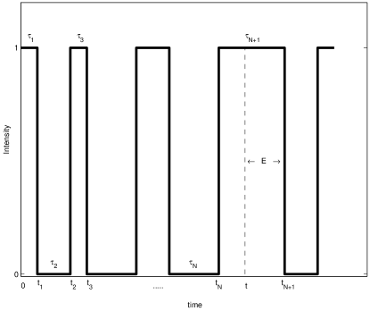
Figure 1: Schematic temporal evolution of the dichotomous intensity process.

We denote the Laplace transform of $\psi_{\pm}(t)$ using

$$\hat{\psi}_{\pm}(s)=\int_{0}^{\infty}\psi_{\pm}(t)e^{-st}\textrm{d}t.$$ (3)

We will classify behaviors of observables of interest using the small $s$ expansion of $\psi_{\pm}\left(s\right)$. We will consider:
(i) Case 1 PDFs with finite mean on and off times, whose Laplace transform in the limit $s\rightarrow 0$ satisfies:

$$\hat{\psi}_{\pm}(s)=1-s\tau_{\pm}+\cdots.$$ (4)

Here $\tau_{+}$ $(\tau_{-})$ is the average on (off) time. For example exponentially distributed on and off times,

$$\hat{\psi}_{\pm}(s)=\frac{1}{1+s\tau_{\pm}},$$ (5)

belong to this class of PDFs.
(ii) Case 2 PDFs with infinite mean on and off times, namely PDFs with power law behavior satisfying

$$\psi_{\pm}\propto t^{-1-\alpha_{\pm}}\,\,\,\,\,\,\,\,\,\,\,\,\alpha_{-}<\alpha_{+}<1,$$ (6)

in the limit of long times. The small $s$ behavior of these family of functions satisfies

$$\hat{\psi}_{\pm}(s)=1-A_{\pm}s^{\alpha_{\pm}}+\cdots$$ (7)

where $A_{\pm}$ are parameters which have units of time^α. We will also consider cases where on times have finite mean $(\alpha_{+}=1)$ while the off mean time diverges $(\alpha_{-}<1)$ since this situation describes behavior of uncapped QD Oijen .
(iii) Case 3 PDFs with infinite mean with $\alpha_{+}=\alpha_{-}=\alpha$

$$\hat{\psi}_{\pm}(s)=1-A_{\pm}s^{\alpha}+\cdots$$ (8)

Note that Brokmann et al. Brokmann report that for CdSe dots, $\alpha_{+}=0.58\pm 0.17$, and $\alpha_{-}=0.48\pm 0.15$, hence within error of measurement, $\alpha\simeq 0.5$.
(iv) In Sec. VII.4 we will briefly consider the behavior of the correlation function for defected $\psi_{-}(t)$.

II.1 Physical Meaning of $\psi_{\pm}(t)$

As mentioned in Introduction, and following Ref. EfrosRosen97 , we assume that a charged (neutral) uncapped NC is in state off (on), respectively. Physically, for charged NC, Auger non-radiative decay time of a laser excited electron-hole pair, is much faster than the radiative time of the electron-hole pair Shimuzu . Hence a charged NC is in off state. The physical mechanism responsible for the power law blinking (i.e. charging) behavior of NCs is still unclear. Models based on trapping of charge carriers in the vicinity of the NC, and fluctuating barrier concepts were suggested in Kuno ; Ken ; Oijen . Here we will emphasize an alternative simple picture based on diffusion concepts. Before further experiments are performed, it is impossible to say if the simple picture we consider here works better or worse than other approaches.

We note that the simplest diffusion controlled chemical reaction $A+B\rightleftharpoons AB$, where $A$ is fixed in space, can be used to explain some of the observed behavior on the uncapped NCs. As mentioned the latter exhibit exponential distribution of on times and power law distribution of off times. The on times follow standard exponential kinetics corresponding to an ionization of a neutral NC (denoted as AB). A model for this exponential behavior was given already in EfrosRosen97 . Once the NC is ionized ($A+B$ state) we assume the ejected charge carrier exhibits a random walk on the surface of the NC or in the bulk. This part of the problem is similar to Onsager’s classical problem of an ion pair escaping neutralization (see e.g., HongNoolandi78 ; SanoTachiya79 ). The survival probability in the off state for time t, $S_{-}(t)$ is related to the off time distribution via $S_{-}(t)=1-\int_{0}^{t}\psi_{-}(\tau)d\tau$, or

$$\psi_{-}(t)=-\frac{dS_{-}(t)}{dt}.$$ (9)

It is well known that in three dimensions survival probability decays like $t^{-1/2}$, the exponent 1/2 is close to the exponent measured in the experiments. In infinite domain the decay is not to zero, but the 1/2 appears in many situations, for finite and infinite systems, in completely and partially diffusion controlled recombination, in different dimensions, and can govern the leading behavior of the survival probability for orders of magnitude in time SanoTachiya79 ; NadlerStein91 ; NadlerStein96 . In this picture the exponent $1/2$ does not depend on temperature, similar to what is observed in experiment. We note that it is possible that instead of the charge carrier executing the random walk, diffusing lattice defects which serve as a trap for charge carrier are responsible for the blinking behavior of the NCs.

One of the possible physical pictures explaining blinking of capped NCs can be based on diffusion process, using a variation of a three state model of Oijen . As mentioned in Introduction, for this case power law distribution of on and off times are observed. In particular, neutral capped NC will correspond to state on (as for uncapped NCs). However, capped NC can remain on even in the ionized state. We assume that the ionized capped NC can be found in two states: (i) the charge remaining in the NC can be found in center of NC (possibly a de-localized state), (ii) charge remaining in the NC can be trapped in vicinity of capping. For case (i) the NC will be in state off, for case (ii) the NC will be in state on. The main idea is that the rate of Auger nonradiative recombination EfrosRosen97 of consecutively formed electron-hole pairs will drop for case (ii) but not for case (i). We note that capping may increase effective radius of the NC, or provide trapping sites for the hole (e.g., recent studies by Lifshitz et al. Lifshitz04 demonstrate that coating of NCs creates trapping sites in the interface). Thus the off times occur when the NC is ionized and the hole is close to the center, these off times are slaved to the diffusion of the electron. While on times occur for both a neutral NC and for charged NC with the charge in vicinity of capping, the latter on times are slaved to the diffusion of the electron. In the case of power law off time statistics this model predicts same power law exponent for the on times, because both of them are governed by the return time of the ejected electron.

The main point we would like to emphasize is that several simple mechanisms might be responsible for the power law statistics, and hence aging correlation functions in single molecule experiments may turn out to be wide spread. Beyond single molecule spectroscopy we note that certain single ion channels NadlerStein91 ; GoychukHanggi01 ; GoychukHanggi02 , deterministic diffusion in chaotic systems ZK , the sign of magnetization of spin systems at criticality GL , all exhibit intermittency behavior, and the correlation function we obtain here might be useful also in other fields. Hence we don’t restrict our attention to the exponent 1/2, as there are indications for other values of $\alpha$ between 0 and 1, and the analysis hardly changes.

II.2 Definition of Correlation Functions

Since the process under investigation is non-ergodic, and since measurements are made on a single molecule level, care must be taken in the definition of averages. From a single trajectory (ST) of $I(t)$, recorded in a time interval $(0,T)$, we may construct the time average correlation function

$$C_{ST}(T,t^{\prime})=\frac{\int_{0}^{T-t^{\prime}}I(t+t^{\prime})I(t)\textrm{d}t}{T-t^{\prime}}.$$ (10)

On the other hand we may generate many intensity trajectories one at a time, to obtain $C(t,t^{\prime})$ and $g^{(2)}(t,t^{\prime})$. We call $C(t,t^{\prime})$ single particle averaged correlation function. For non-ergodic processes $C_{ST}(T,t^{\prime})\neq C(t,t^{\prime})$ even in the limit of large $t$ and $T$. Moreover for non-ergodic processes, even in the limit of $T\rightarrow\infty$, $C_{ST}(T,t^{\prime})$ is a random function which varies from one sample of $I(t)$ to another.

We stress that the single particle averaged correlation function is not the correlation function obtained from measurement of an ensemble of particles. To see this consider the intensity of $N$ blinking NCs,

$$\tilde{I}_{N}=\sum_{j=1}^{N}I_{j}(t)$$ (11)

and $j$ is an index of the particle number. The corresponding normalized correlation function is

$$G^{(2)}(t,t^{\prime})=\frac{\langle\tilde{I}_{N}(t)\tilde{I}_{N}(t+t^{\prime})\rangle}{\langle\tilde{I}_{N}(t)\rangle\langle\tilde{I}_{N}(t+t^{\prime})\rangle}.$$ (12)

If the blinking behavior of individual NCs is independent, but statistically identical,

$$G^{(2)}(t,t^{\prime})=\frac{N\langle I(t)I(t+t^{\prime})\rangle+N(N-1)\langle I(t)\rangle\langle I(t+t^{\prime})\rangle}{N^{2}\langle I(t)\rangle\langle I(t+t^{\prime})\rangle}.$$ (13)

Clearly for $N=1$ we obtain the correlation function $C(t,t^{\prime})$ in Eq. (1), while for $N\rightarrow\infty$ the intensity does not fluctuate at all (as well known). Hence while we consider here average over an ensemble of trajectories, we are not reconstructing the correlation function obtained from a measurement of a large number of NCs. Our theory is valid only for single molecule measurements, and the aging behavior of the normalized correlation function cannot be obtained from macroscopic measurement.

III Number of Jump Events Between $0$ and $t$

In this Section we investigate basic statistical properties of the on-off process.

The probability of $n$ transitions (either off $\rightarrow$ on or on $\rightarrow$ off) between times 0 and t is

$$P_{t}(n)\equiv P(0,t,n)=\langle\theta\left(t_{n}<t<t_{n+1}\right)\rangle$$ (14)

where $\theta(t_{n}<t<t_{n+1})$ is 1 if the event in the parenthesis occurs; otherwise it is zero. Laplace transforming Eq. (14) with respect to t yields

$$\hat{P}_{s}(n)=\langle\int_{t_{n}}^{t_{n+1}}\textrm{d}te^{-st}\rangle=\langle e^{-st_{n}}\left(\frac{1-e^{-s\tau_{n+1}}}{s}\right)\rangle.$$ (15)

A simple calculation using $t_{n}=\sum_{i=1}^{n}\tau_{i}$ yields

$$\hat{P}_{s}\left(n\right)=\left\{\begin{array}[]{ll}\left[\hat{\psi}_{+}\left(s\right)\hat{\psi}_{-}\left(s\right)\right]^{n/2}\frac{1-\hat{\psi}_{+}\left(s\right)}{s}&n\,\,\,\,\,\,\mbox{even}\\ &\\ \left[\hat{\psi}_{+}\left(s\right)\right]^{\frac{n+1}{2}}\left[\hat{\psi}_{-}\left(s\right)\right]^{\frac{n-1}{2}}\frac{1-\hat{\psi}_{-}\left(s\right)}{s}&n\,\,\,\,\,\,\mbox{odd}\end{array}\right.$$ (16)

To derive Eq. (16) we used the initial condition that the state of the process at $t=0$ is $+$. Eq. (16) satisfies the normalization condition $\sum_{n=0}^{\infty}\hat{P}_{s}(n)=1/s$.

III.1 Mean number of renewals $\langle n\rangle$

Using Eq. (16) the mean number of transitions is in Laplace $t\rightarrow s$ space

$$\langle\hat{n}(s)\rangle=\sum_{n=0}^{\infty}n\hat{P}_{s}(n)=\frac{\hat{\psi}_{+}(s)\left[1+\hat{\psi}_{-}(s)\right]}{s\left[1-\hat{\psi}_{-}(s)\hat{\psi}_{+}(s)\right]}.$$ (17)

Using Eqs. (4, 7, 8), the small $s$ expansion of Eq. (17), and then inverting to time domain we get the long time behavior

$$\langle n(t)\rangle\sim\left\{\begin{array}[]{cc}\frac{2t}{\tau_{+}+\tau_{-}}&\mbox{case}\,\,\,\,1\\ &\\ \frac{2t^{\alpha_{-}}}{A_{-}\Gamma\left(1+\alpha_{-}\right)}&\mbox{case}\,\,\,\,2\\ &\\ \frac{2t^{\alpha}}{\left(A_{+}+A_{-}\right)\Gamma\left(1+\alpha\right)}&\mbox{case}\,\,\,\,3.\end{array}\right.$$ (18)

III.2 Asymptotes of $P_{t}(n)$

For narrow PDFs, i.e. case 1, and for long times we obtain from Eqs. (4, 16)

$$P_{t}(n)\simeq\left\{\begin{array}[]{cc}\frac{\langle\tau_{+}\rangle}{\langle\tau_{+}\rangle+\langle\tau_{-}\rangle}\delta\left(\frac{n}{2}-\frac{t}{\langle\tau_{+}\rangle+\langle\tau_{-}\rangle}\right)&n\,\,\,\,\,\,\,\,\mbox{even}\\ &\\ \frac{\langle\tau_{-}\rangle}{\langle\tau_{+}\rangle+\langle\tau_{-}\rangle}\delta\left(\frac{n+1}{2}-\frac{t}{\langle\tau_{+}\rangle+\langle\tau_{-}\rangle}\right)&n\,\,\,\,\,\,\,\,\mbox{odd}\end{array}\right.$$ (19)

To obtain this result we used the small $s$ expansion of Eq. (16) and then a simple Laplace inversion. We neglected the fluctuations in this treatment, the latter are expected to be Gaussian in the long time limit.

For broad PDFs satisfying $\alpha_{+}=\alpha_{-}=\alpha$, case $3$, we find

$$\hat{P}_{s}(n)\sim A_{\pm}s^{\alpha-1}e^{-k\left(A_{+}+A_{-}\right)s^{\alpha}}$$ (20)

where $k=n/2$ and $A_{\pm}=A_{+}$ for $n$ even, while $k=(n+1)/2$ and $A_{\pm}=A_{-}$ for $n$ odd. Inverting to the time domain we find

$$P_{t}(n)\sim\frac{A_{\pm}}{\alpha}\frac{t}{(A_{+}k+A_{-}k)^{1/\alpha+1}}l_{\alpha}\left[\frac{t}{\left(A_{+}k+A_{-}k\right)^{1/\alpha}}\right].$$ (21)

where $l_{\alpha}(t)$ is the one sided Lévy stable PDF whose Laplace pair is $\exp(-s^{\alpha})$.

For case $2$, with $\alpha_{-}<\alpha_{+}$, we get

$$\hat{P}_{s}(n)\sim A_{-}\exp\left(-A_{-}ks^{\alpha_{-}}\right)$$ (22)

for $k=n/2$ and $n$ even. The probability of finding an odd $n$ in this limit is zero. This is expected since the off times are much longer than the on times, in statistical sense. Thus for long times we have

$$P_{t}(n)\sim\frac{A_{-}}{\alpha_{-}}\frac{t}{(A_{-}k)^{1/\alpha_{-}+1}}l_{\alpha_{-}}\left[\frac{t}{\left(A_{-}k\right)^{1/\alpha_{-}}}\right]$$ (23)

and $n$ is even.

IV Forward Recurrence Time

The time $E=t_{N+1}-t$ is called the forward recurrence time. The times (see Fig. 1) $t_{N+1}$ and $t_{N}$ are defined in such a way that $t_{N}<t<t_{N+1}$, hence also $N$ is a random variable. Let $f_{t}(E)$ be the probability density function of the random variable $E$. The subscript $t$ in $f_{t}(E)$ indicates that $t$ is a parameter, while $E$ is a random variable. Generally the PDF of $E$ depends on how old the process is, namely on $t$. A process is said to exhibit statistical aging if even in the limit of $t\rightarrow\infty$, $f_{t}(E)$ depends on $t$. The PDF $f_{t}(E)$ is important for the calculation of the aging correlation function.

We consider the joint PDF

$$\textrm{f}_{t}(E,N)=\langle\delta\left(E-t_{N+1}+t\right)\theta\left(t_{N}<t<t_{N+1}\right)\rangle.$$ (24)

Later we will sum over $N$ to obtain $f_{t}(E)$. We consider the double Laplace transform $\mathcal{L}$ of Eq. (24) with $t\rightarrow s$ and $E\rightarrow u$

$$\mathcal{L}_{t,E}\left\{\textrm{f}_{t}(E,N)\right\}=$$

$$=\langle\int_{t_{N}}^{t_{N+1}}\textrm{d}t\int_{0}^{\infty}\textrm{d}Ee^{-st-uE}\delta\left(E-t_{N+1}+t\right)\rangle$$

$$=\langle e^{-ut_{N+1}}\int_{t_{N}}^{t_{N+1}}e^{-(s-u)t}\textrm{d}t\rangle$$

$$=\langle e^{-ut_{N+1}}\frac{e^{-(s-u)t_{N+1}}-e^{-(s-u)t_{N}}}{u-s}\rangle.$$ (25)

For even $N$ we use the averages

$$\langle e^{-st_{N+1}}\rangle=\left[\hat{\psi}_{+}\left(s\right)\right]^{\frac{N}{2}+1}\left[\hat{\psi}_{-}\left(s\right)\right]^{\frac{N}{2}},$$

$$\langle e^{-st_{N}}\rangle=\left[\hat{\psi}_{+}\left(s\right)\hat{\psi}_{-}\left(s\right)\right]^{\frac{N}{2}},$$

$$\langle e^{-u(t_{N+1}-t_{N})}\rangle=\hat{\psi}_{+}\left(u\right),$$

and find

$$\hat{\textrm{f}}_{s}(u,N)=\frac{\left[\hat{\psi}_{+}\left(s\right)\psi_{-}\left(s\right)\right]^{N/2}\left[\hat{\psi}_{+}(s)-\hat{\psi}_{+}(u)\right]}{u-s}.$$ (26)

In similar way we obtain for $N$ odd

$$\hat{\textrm{f}}_{s}(u,N)=\frac{\left[\hat{\psi}_{+}\left(s\right)\psi_{-}\left(s\right)\right]^{\frac{N-1}{2}}\left[\hat{\psi}_{-}(s)-\hat{\psi}_{-}(u)\right]\hat{\psi}_{+}(s)}{u-s}.$$ (27)

Note that $\hat{\textrm{f}}_{s}(u,N)$ is the double Laplace transform of $\hat{\textrm{f}}_{t}(E,N)$, while $\hat{\psi}_{\pm}(s)$ and $\hat{\psi}_{\pm}(u)$ are single Laplace transforms. Summing $\hat{\textrm{f}}_{s}(u,N)$ over $N$ we obtain the double Laplace transform of $f_{t}(E)$

$$\hat{f}_{s}(u)=\frac{\left[\hat{\psi}_{+}\left(s\right)-\hat{\psi}_{+}\left(u\right)\right]+\hat{\psi}_{+}(s)\left[\hat{\psi}_{-}(s)-\hat{\psi}_{-}\left(u\right)\right]}{\left(u-s\right)\left[1-\hat{\psi}_{+}(s)\hat{\psi}_{-}(s)\right]}.$$ (28)

For $\hat{\psi}_{+}(s)=\hat{\psi}_{-}(s)$ Eq. (28) reduces to Eq. $6.2$ in GL .

IV.1 Limiting cases for $f_{t}(E)$

We now analyze the long time $t\rightarrow\infty$ behavior of $f_{t}(E)$. In this case we expect that an equilibrium PDF for $f_{t}(E)$ will emerge. This equilibrium is related to stationarity, ergodicity, and aging as we will show.

We consider narrow distributions, i.e. case $1$ first. Taking the limit $s\rightarrow 0$ of Eq. (28), corresponding to $t\rightarrow\infty$ and find

$$\hat{f}_{s}(u)\sim\frac{1-\hat{\psi}_{+}\left(u\right)}{su\left(\tau_{+}+\tau_{-}\right)}+\frac{1-\hat{\psi}_{-}\left(u\right)}{su\left(\tau_{+}+\tau_{-}\right)}.$$ (29)

The Laplace $s\rightarrow t$ and $u\rightarrow E$ inversion of this equation is immediate

$$f_{t}(E)=\frac{\int_{E}^{\infty}\psi_{+}(t^{\prime})\textrm{d}t^{\prime}}{\tau_{+}+\tau_{-}}+\frac{\int_{E}^{\infty}\psi_{-}(t^{\prime})\textrm{d}t^{\prime}}{\tau_{+}+\tau_{-}},$$ (30)

a behavior which is valid in the limit of long time $t$ (and independent of it). Note that the first (second) term on the right hand side of the equation, corresponds to trajectories with even (odd) number of steps. One can show that in the limit of long times probability of finding the process in state $\pm$ is

$$\lim_{t\rightarrow\infty}P_{\pm}(t)=\frac{\tau_{\pm}}{\tau_{+}+\tau_{-}},$$ (31)

as might be expected. In the special case of $\psi_{-}=\psi_{+}$ we obtain a well known equation Feller which has several applications in theory of random walks e.g. Haus . The important point to notice is that in the limit of large time $t$, and when average times $\tau_{\pm}$ are finite, an equilibrium is obtained which does not depend on $t$.

We now consider broad distributions, with diverging averaged on and off times, case $2$. In the limit of small $s$ and small $u$, with their ratio finite

$$\hat{f}_{s}(u)\sim\frac{u^{\alpha_{-}}-s^{\alpha_{-}}}{(u-s)s^{\alpha_{-}}}.$$ (32)

The investigation of this equation yields the long time $t$ behavior

$$f_{t}(E)\sim d_{t}(E),$$ (33)

where $d_{t}(E)$ is Dynkin’s function

$$d_{t}(E)=\frac{\sin(\pi\alpha_{-})}{\pi}\frac{t^{\alpha_{-}}}{E^{\alpha_{-}}(t+E)}.$$ (34)

From Eqs. (32,33) we learn that unlike case 1, the PDF of $E$ depends on time $t$ even in the long time limit. Eq. (34) was obtained by Dynkin Feller ; Dynkin as a limit theorem for renewal processes with a single waiting time PDF. Here we showed that for a two state process the details on $\alpha_{+}$ and $A_{+}$ are not important in the long time limit. This is expected, the off (i.e. minus) times are much longer than the on (i.e. plus) times in statistical sense, and hence our results in the long time limit are not sensitive to the details of $\psi_{+}(t)$. In the same spirit it can be shown that in the limit of long time $t$, and with probability one, the process is found in state minus.

Finally for case $3$ where $\alpha_{+}=\alpha_{-}<1$, we find that Eqs. (32,33) are still valid. However now probability of finding the process in state $\pm$ is given by

$$P_{\pm}\equiv\lim_{t\rightarrow\infty}P_{\pm}(t)=\frac{A_{\pm}}{A_{+}+A_{-}}.$$ (35)

IV.2 Joint PDFs for Forward Recurrence time

It will turn out important to define the joint PDFs of time $E$ provided that process is in state plus or state minus at time $t$. We denote these PDFs with $f_{t}(E,\pm)$ and the corresponding double Laplace transform $\hat{f}_{s}(u,\pm)$. Since the start of process is state $+$ at time $t=0$, we get using Eq. (26)

$$\hat{f}_{s}(u,+)=\sum_{N=0,N\mbox{ even}}^{\infty}\hat{\textrm{f}}_{s}(u,N)=$$

$$\frac{\hat{\psi}_{+}(s)-\hat{\psi}_{+}(u)}{(u-s)\left[1-\hat{\psi}_{+}(s)\hat{\psi}_{-}(s)\right]}.$$ (36)

and using Eq. (27)

$$\hat{f}_{s}(u,-)=\sum_{N=0,N\mbox{ odd}}^{\infty}\hat{\textrm{f}}_{s}(u,N)=$$

$$\frac{\hat{\psi}_{+}(s)\left[\hat{\psi}_{-}(s)-\hat{\psi}_{-}(u)\right]}{(u-s)\left[1-\hat{\psi}_{+}(s)\hat{\psi}_{-}(s)\right]}.$$ (37)

Note that

$$\hat{f}_{s}(u)=\hat{f}_{s}(u,-)+\hat{f}_{s}(u,+).$$ (38)

The probability of finding the particle in state $+$ when $t\rightarrow\infty$ is

$$\lim_{t\rightarrow\infty}P_{+}=\lim_{t\rightarrow\infty}\int_{0}^{\infty}f_{t}(E,+)\textrm{d}E,$$ (39)

provided that the limit exists. For example for case 1 it is easy obtain from Eq. (39) the result in Eq. (31).

The limiting PDFs $f_{t}(E,\pm)$ are obtained in double Laplace space by considering the small $s$ (and small u for cases 2 and 3) limit. They are

$$\hat{f}_{s}(u,\pm)\sim\left\{\begin{array}[]{cc}\frac{1-\hat{\psi}_{\pm}(u)}{us(\tau_{+}+\tau_{-})}&\mbox{case}\,\,1\\ &\\ \frac{A_{\pm}}{A_{+}+A_{-}}\frac{u^{\alpha}-s^{\alpha}}{(u-s)s^{\alpha}}&\mbox{case}\,\,3.\end{array}\right.$$ (40)

For case $2$ we find in this limit $\hat{f}_{s}(u,+)=0$, i.e. probability of finding the particle in state $+$ is zero, and

$$\hat{f}_{s}(u,-)=\frac{u^{\alpha}-s^{\alpha}}{(u-s)s^{\alpha}}.$$ (41)

The double inverse Laplace transform of this equation is given in Eq. (34).

V Number of Renewals Between Two Times

We now calculate $P(t,t+t^{\prime},n)$ the probability of number of renewals $n$ between time $t$ and time $t+t^{\prime}$. Obviously the process is generally not stationary and the information on $P(0,t^{\prime},n)$, obtained in Sec. III, is not sufficient for the determination of $P(t,t+t^{\prime},n)$. We now classify the trajectories according to the state of the process (i.e., $+$ or $-$) at times $t$ and $t+t^{\prime}$. It will turn out that the intensity trajectories, when the process is in state $+$ at time $t$ and state $+$ at time $t+t^{\prime}$, are those which are important for the calculation of the correlation function.

The probability of not making a jump in time interval $t,t+t^{\prime}$, when the process is in state $+$ at time $t$ and state $+$ at time $t+t^{\prime}$ is

$$P_{++}(t,t+t^{\prime},0)=\int_{t^{\prime}}^{\infty}f_{t}(E,+)\textrm{d}E.$$ (42)

The probability of finding $n>0$ transition events in time interval $t,t+t^{\prime}$, when state of process at time $t$ is $+$ and state of process is $t+t^{\prime}$ is also $+$

$$\mathcal{L}_{t^{\prime}}P_{++}(t,t+t^{\prime},n)=$$

$$\hat{f}_{t}(u,+)\hat{\psi}_{-}(u)\left[\hat{\psi}_{+}(u)\hat{\psi}_{-}(u)\right]^{\frac{n}{2}-1}\frac{1-\hat{\psi}_{+}(u)}{u},$$ (43)

where $n>0$ is even, and $u$ is the Laplace conjugate of $t^{\prime}$. Note that Eq. (43) depends on $t$ through $\hat{f}_{t}(u,+)$. The other combinations, e.g. $P_{+-}(t,t+t^{\prime},n)$, are given in Appendix A, as well as $P(t,t+t^{\prime},n)$.

VI Mean Intensity of on-off process

The averaged intensity $\langle I(t)\rangle$ for the process switching between 1 and 0 and starting at 1 is now considered. In Laplace $t\rightarrow s$ space it is easy to show that

$$\left\langle\hat{I}(s)\right\rangle=\frac{1-\hat{\psi}_{+}(s)}{s}\cdot\frac{1}{1-\hat{\psi}_{+}(s)\hat{\psi}_{-}(s)}.$$ (44)

One method to obtain this equation is to note that $\langle I(t)\rangle=\mbox{Prob}[I(t)=1]$, hence

$$\left\langle\hat{I}(s)\right\rangle=\int_{0}^{\infty}f_{s}(E,+)\textrm{d}E,$$ (45)

and therefore the $u\rightarrow 0$ limit of Eq. (36) yields Eq. (44).

The Laplace $s\rightarrow t$ inversion of Eq. (44) yields the mean intensity $\langle I(t)\rangle$. Using small $s$ expansions of Eq. (44), we find in the limit of long times

$$\langle I(t)\rangle\sim\left\{\begin{array}[]{cc}\frac{\tau_{+}}{\tau_{+}+\tau_{-}}&\mbox{case}\,\,\,\,1\\ &\\ \frac{A_{+}t^{\alpha_{-}-\alpha_{+}}}{A_{-}\Gamma\left(1+\alpha_{-}-\alpha_{+}\right)}&\mbox{case}\,\,\,\,2\\ &\\ \frac{A_{+}}{A_{+}+A_{-}}&\mbox{case}\,\,\,\,3.\end{array}\right.$$ (46)

If the on times are exponential, as in Eq. (5) then

$$\left\langle\hat{I}(s)\right\rangle=\frac{\tau_{+}}{1+s\tau_{+}-\psi_{-}(s)}.$$ (47)

This case corresponds to the behavior of the uncapped NCs. The expression in Eq. (47), and more generally, the case $\alpha_{-}<\alpha_{+}=1$ leads for long time t to

$$\left\langle I(t)\right\rangle\sim\frac{\tau_{+}t^{\alpha_{-}-1}}{A_{-}\Gamma(\alpha_{-})}.$$ (48)

For exponential on and off time distributions Eq. (5), we obtain the exact solution

$$\left\langle I(t)\right\rangle=\frac{\tau_{-}\exp\left[-t\left(\frac{1}{\tau_{-}}+\frac{1}{\tau_{+}}\right)\right]+\tau_{+}}{\tau_{-}+\tau_{+}}.$$ (49)

Remark For the case $\alpha_{+}<\alpha_{-}<1$, corresponding to a situation where on times are in statistical sense much longer then off times, $\langle I(t)\rangle\sim 1$.

VII Aging Correlation Function of on-off process

We are now able to calculate the correlation function $C(t,t^{\prime})=\langle I(t)I(t+t^{\prime})\rangle$. We consider the process $I(t)$ as jumping between state on with $I(t)=+1$ and state off $I(t)=0$. The symmetric case where $I(t)$ jumps between the states $I(t)=-1$ or $I(t)=-1$, is discussed in Appendix B. We assume that sojourn times in state on (off) are described by $\psi_{+}(t)$ ($\psi_{-}(t)$), respectively. Contributions to the correlation function arise only from trajectories with $I(t)=1$ and $I(t+t^{\prime})=1$, meaning that only the $++$ trajectories, in Eq. (43) contribute to the correlation function. Summing Eq. (43) over even $n>0$, and using Eq. (42) for $n=0$, we find

$$\hat{C}(t,u)=\frac{\hat{f}_{t}(u=0,+)-\hat{f}_{t}(u,+)}{u}$$

$$+\hat{f}_{t}(u,+)\frac{\hat{\psi}_{-}(u)\left[1-\hat{\psi}_{+}(u)\right]}{u\left[1-\hat{\psi}_{-}(u)\hat{\psi}_{+}(u)\right]},$$ (50)

where $u$ is the Laplace conjugate of $t^{\prime}$. We see that the correlation function generally depends on time $t$.

VII.1 Case 1

For case $1$ with finite $\tau_{+}$ and $\tau_{-}$, and in the limit of long times $t$, we find

$$\lim_{t\rightarrow\infty}\hat{C}(t,u)=$$

$$\frac{1}{u}\frac{\tau_{+}}{\tau_{+}+\tau_{-}}\left\{1-\frac{\left[1-\hat{\psi}_{+}(u)\right]\left[1-\hat{\psi}_{-}(u)\right]}{\tau_{+}u\left[1-\hat{\psi}_{-}(u)\hat{\psi}_{+}(u)\right]}\right\}$$ (51)

This result was obtained by Verberk and Orrit Verberk and it is seen that the correlation function depends asymptotically only on $t^{\prime}$(since u is Laplace pair of $t^{\prime}$). Namely, when average on and off times are finite the system does not exhibit aging. If both $\psi_{+}(t)$ and $\psi_{-}(t)$ are exponential then the exact result is

$$\begin{array}[]{ccc}C(t,t^{\prime})&=&\frac{\tau_{-}\exp\left[-t\left(\frac{1}{\tau_{-}}+\frac{1}{\tau_{+}}\right)\right]+\tau_{+}}{\tau_{-}+\tau_{+}}\\ \\ &\times&\frac{\tau_{-}\exp\left[-t^{\prime}\left(\frac{1}{\tau_{-}}+\frac{1}{\tau_{+}}\right)\right]+\tau_{+}}{\tau_{-}+\tau_{+}}\end{array}$$

and $C(t,t^{\prime})$ becomes independent of t exponentially fast as t grows.

VII.2 Case 2

We consider case $2$, however limit our discussion to the case $\alpha_{+}=1$ and $\alpha_{-}<1$. As mentioned this case corresponds to uncapped NCs where on times are exponentially distributed, while off times are described by power law statistics. Using the exact solution Eq. (50) we find asymptotically, when both both t and $t^{\prime}$ are large:

$$C(t,t^{\prime})\sim\left(\frac{\tau_{+}}{A_{-}}\right)^{2}\frac{\left(tt^{\prime}\right)^{\alpha_{-}-1}}{\Gamma^{2}\left(\alpha_{-}\right)}.$$ (52)

Unlike case $1$ the correlation function approaches zero when $t\rightarrow\infty$, since when $t$ is large we expect to find the process in state off. Using Eq. (48), the asymptotic behavior of the normalized correlation function Eq. (2) is

$$g^{(2)}(t,t^{\prime})\sim\left(1+\frac{t}{t^{\prime}}\right)^{1-\alpha_{-}}.$$ (53)

We see that the correlation functions Eqs. (52, 53) exhibit aging, since they depend on the age of the process $t$.

Considering the asymptotic behavior of $C(t,t^{\prime})$ for large t, but small $t^{\prime}$, yields in the limit of $s\ll u,\,s\ll u\hat{\psi}(u)$

$$\hat{C}(t,u)\approx$$

$$\frac{1}{u}\frac{\tau_{+}}{A_{-}\Gamma(\alpha_{-})t^{1-\alpha_{-}}}\left\{1-\frac{\left[1-\hat{\psi}_{+}(u)\right]\left[1-\hat{\psi}_{-}(u)\right]}{\tau_{+}u\left[1-\hat{\psi}_{-}(u)\hat{\psi}_{+}(u)\right]}\right\}.$$ (54)

This equation is similar to Eq. (51), especially if we notice that the “effective mean” time of state off until total time t scales as $A_{-}t^{1-\alpha_{-}}$. Despite assumptions of $s\ll u,\,s\ll u\hat{\psi}(u)$ in the derivation of Eq. (54), it also reproduces the result Eq. (52) and hence is applicable for any u (and thus $t^{\prime}$) as long as t is large enough.

For the special case, where on times are exponentially distributed, the correlation function C is a product of two identical expressions for all t and $t^{\prime}$:

$$\hat{C}(s,u)=\frac{\tau_{+}}{1+s\tau_{+}-\psi_{-}(s)}\cdot\frac{\tau_{+}}{1+u\tau_{+}-\psi_{-}(u)},$$ (55)

where s (u) is the Laplace conjugate of t (t’) respectively. Comparing to Eq. (47) we obtain

$$C(t,t^{\prime})=\langle I(t)\rangle\langle I(t^{\prime})\rangle,$$ (56)

and for the normalized correlation function

$$g^{(2)}(t,t^{\prime})=\frac{\left\langle I(t^{\prime})\right\rangle}{\left\langle I(t+t^{\prime})\right\rangle}.$$ (57)

Eqs. (57, 56) are important since they show that measurement of mean intensity $\langle I(t)\rangle$ yields the correlation functions, for this case. While our derivation of Eqs. (57, 56) is based on the assumption of exponential on times, it is valid more generally for any $\psi_{+}(t)$ with finite moments, in the asymptotic limit of large $t$ and $t^{\prime}$. To see this note that Eqs. (52, 48) yield $C(t,t^{\prime})\sim\langle I(t)\rangle\langle I(t^{\prime})$.

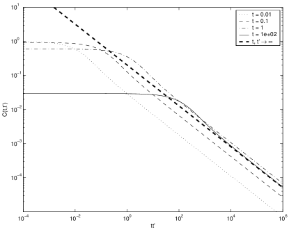
Figure 2: Exact $C(t,t^{\prime})$ for Case $2$: exponential on times and power law off times with $\alpha_{-}=0.4$. We use $\hat{\psi}_{+}(s)=1/(1+s)$ and $\hat{\psi}_{-}(s)=1/(1+s^{0.4})$ and numerically obtain the correlation function. For each curve in the figure we fix the time $t$. The process starts in the state $on$. Thick dashed straight line shows the asymptotic behavior Eq. (52). For short times ($t^{\prime}<1$ for our example) we observe the behavior $C(t,t^{\prime})\sim C(t,0)=\langle I(t)\rangle$, the correlation function is flat.

In Fig. 2 we compare the asymptotic result (52) with exact numerical double Laplace inversion of the correlation function. We use exponential PDF of on times $\psi_{+}(s)=1/(1+s)$, and power law distributed off times: $\hat{\psi}_{-}(s)=\hat{\psi}_{-}(s)=1/(1+s^{0.4})$ corresponding to $\alpha_{-}=0.4$. Convergence to asymptotic behavior is observed.

Remark For fixed $t$ the correlation function in Eq. (52) exhibits a $(t^{\prime})^{\alpha_{-}-1}$ decay. A $(t^{\prime})^{\alpha_{-}-1}$ decay of an intensity correlation function was reported in experiments of Orrit’s group Oijen for uncapped NCs (for that case $\alpha_{-}=0.65\pm 0.2$). However, the measured correlation function is a time averaged correlation function Eq. (10) obtained from a single trajectory. In that case the correlation function is independent of $t$, and hence no comparison between theory and experiment can be made yet.

VII.3 Case 3

We now consider case $3$, and for long t and $t^{\prime}$ we find

$$C(t,t^{\prime})=P_{+}-P_{+}P_{-}\frac{\sin\pi\alpha}{\pi}B\left(\frac{1}{1+t/t^{\prime}};1-\alpha,\alpha\right)$$ (58)

with $P_{\pm}$ given by Eq. (35) and where

$$B(z;a,b)=\int_{0}^{z}x^{a-1}(1-x)^{b-1}dx$$

is the incomplete beta function. The behavior in this limit does not depend on the detailed shape of the PDFs of the on and off times, besides the parameters $A_{+}/A_{-}$ and $\alpha$ (see also Appendix C). We note that both terms of Eq. (50) contribute to Eq. (58). The appearance of the incomplete beta function in Eq. (58) is related to the concept of persistence. The probability of not switching from state on to state off in a time interval $(t,t+t^{\prime})$, assuming the process is in state on at time $t$, is called the persistence probability. In the scaling limit this probability is found using Eqs. (34, 40):

$$\frac{\sin(\pi\alpha)}{\pi}\int_{t^{\prime}}^{\infty}\frac{t^{\alpha}}{E^{\alpha}(t+E)}\textrm{d}E$$

$$=1-\frac{\sin\pi\alpha}{\pi}B\left(\frac{1}{1+t/t^{\prime}};1-\alpha,\alpha\right)$$ (59)

The persistence implies that long time intervals in which the process does not jump between states on and off, control the asymptotic behavior of the correlation function. The factor $P_{+}$, which is controlled by the amplitude ratio $A_{+}/A_{-}$, determines the expected short and long time $t^{\prime}$ behaviors of the correlation function, namely $C(\infty,0)=\lim_{t\rightarrow\infty}\langle I(t)I(t+0)\rangle=P_{+}$ and $C(\infty,\infty)=\lim_{t\rightarrow\infty}\langle I(t)I(t+\infty)\rangle=(P_{+})^{2}$. With slightly more details the two limiting behaviors are:

$$C(t,t^{\prime})\sim\left\{\begin{array}[]{cc}P_{+}&\,\,\,\frac{t^{\prime}}{t}\ll 1\\ &\\ (P_{+})^{2}+P_{+}\frac{\sin(\pi\alpha)}{\pi\alpha}\left(\frac{t^{\prime}}{t}\right)^{-\alpha}&\,\,\,\frac{t^{\prime}}{t}\gg 1.\end{array}\right.$$ (60)

Using Eq. (46) the normalized intensity correlation function is $g^{(2)}(t,t^{\prime})\sim C(t,t^{\prime})/(P_{+})^{2}$.

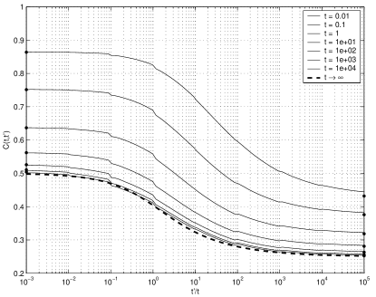
Figure 3: Exact $C(t,t^{\prime})$ for case $3$, when both on and off times are power law distributed with $\alpha=0.4$. We use $\hat{\psi}_{\pm}(s)=1/(1+s^{0.4})$ for different times t increasing from the topmost to the lowermost curves. The dots on the left and on the right show $C(t,0)=\left\langle I(t)\right\rangle$ and $C(t,\infty)=\left\langle I(t)\right\rangle/2$ respectively. The process starts in the state on.

In Fig. 3 we compare the asymptotic result (58) with exact numerical double Laplace inversion of the correlation function for PDFs $\hat{\psi}_{+}(s)=\hat{\psi}_{-}(s)=1/(1+s^{0.4})$. Convergence to Eq. (58) is seen.

Remark For small $t^{\prime}/t$ we get flat correlation functions. Flat correlation functions were observed by Dahan’s group Dahan for capped NCs. However, the measured correlation function is a single trajectory correlation function Eq. (10), and hence no comparison between theory and experiment can be made yet.

VII.4 Defected off time distribution

As mentioned in the Introduction, an off state of uncapped NC corresponds to an ionized NC. Assume that the transition from state on to state off occurs when a charge carrier is ejected into the vicinity of the NC, and then starts to move diffusively in the bulk. If the diffusion process takes place in three dimensions, there is a finite probability that the charge carrier will not return to the NC. In that case the NC remains in state off forever.

Such a situation can be modeled based on defected distribution of off times. In this case we have a non-normalized PDF of off times

$$\int_{0}^{\infty}\psi_{-}(t)dt=Z<1,$$ (61)

the small $s$ expansion of the Laplace transform of $\psi_{-}(t)$ is $\hat{\psi}(s)\approx Z-A_{-}s^{\alpha_{-}}$. $Z$ is the probability of charge carrier to return; this probability was the subject of extensive investigation in the context of first passage time problems Redner .

For large t the mean intensity is

$$\left\langle I(t)\right\rangle\sim\left\{\begin{array}[]{cc}\frac{A_{+}t^{-\alpha_{+}}}{(1-Z)\Gamma(1-\alpha_{+})},&\alpha_{\pm}<1\\ \\ \frac{A_{+}A_{-}t^{-(1+\alpha_{-})}}{(1-Z)^{2}|\Gamma(-\alpha_{-})|},&\,\,\,\alpha_{-}<\alpha_{+}=1.\end{array}\right.$$ (62)

Note that here $\alpha_{-}$ can be smaller, larger or equal to $\alpha_{+}$ when $\alpha_{+}<1$.

Using Eq. (50) we obtain asymptotically, for both t and $t^{\prime}$ large,

$$C(t,t^{\prime})\sim\left\{\begin{array}[]{cc}\frac{A_{+}}{(1-Z)\Gamma(1-\alpha_{+})}(t+t^{\prime})^{-\alpha_{+}},&\alpha_{\pm}<1\\ &\\ \left(\frac{A_{-}A_{+}}{(1-Z)^{2}\Gamma(-\alpha_{-})}\right)^{2}(tt^{\prime})^{-(1+\alpha_{-})},&\alpha_{-}<\alpha_{+}=1.\end{array}\right.$$ (63)

Using Eq. (62) we can relate the intensity correlation function with the mean intensity,

$$C(t,t^{\prime})\sim\left\{\begin{array}[]{cc}\langle I(t+t^{\prime})\rangle,&\alpha_{\pm}<1\\ &\\ \langle I(t)\rangle\langle I(t^{\prime})\rangle,&\,\,\,\alpha_{-}<\alpha_{+}=1.\end{array}\right.$$ (64)

This result shows that for $\alpha_{+}<1$ $\left\langle I(t)I(t+t^{\prime})\right\rangle\simeq\left\langle I(t+t^{\prime})\right\rangle$, independent of the value of $I(t)$. Asymptotic validity of this relation can be explained by noticing that the non-zero contributions to $\left\langle I(t)I(t+t^{\prime})\right\rangle$ come only when both $I(t)$ and $I(t+t^{\prime})$ are equal to 1. However, at long time t, after jumping off there is a negligible probability of being on again for a cumulative time duration comparable with the total time (note that $\left\langle I(t)\right\rangle$ scales as the probability of making no transition off, i.e., of persistence). Hence, the nonzero contributions to $\left\langle I(t+t^{\prime})\right\rangle$ are mainly those staying on from time t, so that almost certainly, if $I(t+t^{\prime})=1$ then also $I(t)=1$ and $\left\langle I(t)I(t+t^{\prime})\right\rangle\simeq\left\langle I(t+t^{\prime})\right\rangle$.

The above argument does not hold in the case of $\alpha_{+}=1$, because now the on times are very short and there is no possibility of staying on persistently for long times. Accordingly, the decay of $\left\langle I(t)\right\rangle$ and $C(t,t^{\prime})$ is much faster here. The leading contributions to $\left\langle I(t)\right\rangle$ and $C(t,t^{\prime})$ in the case of $\alpha_{+}<1$ disappear as $\alpha_{+}\nearrow 1$, due to the pole of the $\Gamma$-function.

VIII Summary

We demonstrated the dependence of the two-time correlation function $C(t,t^{\prime})=\left\langle I(t)I(t+t^{\prime})\right\rangle$ on the times $t$ and $t^{\prime}$. This is in a full contrast to the well-known convergence of the correlation function to the stationary limit which is independent of t. Such a convergence is found when the average on and off times are finite (as shown above for exponential on and off distributions). When these times diverge non-stationary behavior is found. The non-vanishing t-dependence of the correlation function $C(t,t^{\prime})$ is known as aging.

We obtain different modes of aging, yielding dependence of $C(t,t^{\prime})$ on the ratio $t/t^{\prime}$, product $tt^{\prime}$ and the sum $t+t^{\prime}$.
(i) For PDF of on times having finite mean and power law distributed off times with infinite mean, the correlation function asymptotically splits into a product of two identical functions, one of t and the other of $t^{\prime}$ (see Eq. (55)), leading to $tt^{\prime}$ dependence Eq. (52). This case corresponds to the behavior of the uncapped NCs.
(ii) When both on and off times are described by broad distributions, with identical exponents $\alpha_{+}=\alpha_{-}$, the correlation function depends on the ratio $t/t^{\prime}$, Eq. (58). This case corresponds to the capped NCs (within the error of measurement).
(iii) For defected off times and $\alpha_{+}<1$, we find that the correlation function depends on $t+t^{\prime}$, Eq. (63).
(iv) Finally, for stochastic processes with finite on and off times, we recover known behavior, where the correlation function in the scaling limit depends only on $t^{\prime}$, Eq. (51).

In different regimes, the correlation function exhibits either a strong sensitivity on the details of the stochastic process (i.e., on $\psi_{\pm}(t)$), or certain universal features which are now discussed. We also found relations between the correlation function and mean intensity, for several cases.
(i) For PDF of on times having finite mean and power law distributed off times with infinite mean, the correlation function is related to the mean intensity according to $C(t,t^{\prime})\sim\langle I(t)\rangle\langle I(t^{\prime})\rangle$ Eq. (56). For short times $t^{\prime}$ the correlation function depends on the details of $\psi_{\pm}(t)$, Eq. (54).
(ii) When both on and off times are described by broad distributions, with identical exponents $\alpha_{+}=\alpha_{-}$, the persistence probability governs the aging correlation function Eq. (58). This is a universal behavior in the sense that all $\psi_{\pm}(t)$ belonging to this family, yield identical behavior for the correlation function $C(t,t^{\prime})$ in the limit of $t\rightarrow\infty$.
(iii) For defected off times and $\alpha_{+}<1$, we find that the correlation function $C(t,t^{\prime})=\langle I(t+t^{\prime})\rangle$.
(iv) For the standard case, where both the mean on and mean off times are finite, the correlation function depends on the details of $\psi_{\pm}(t)$.

Simple physical explanations for the aging behavior were briefly discussed. Models, discussed previously in the literature, based on diffusion processes, or fluctuating barrier models, or trap models, may all lead to aging behavior of the correlation function. Thus aging behaviors in single molecule spectroscopy may have other applications besides single nano-crystal spectroscopy. The dependence of the correlation function on control parameters like temperature and laser intensity can be used to distinguish between the microscopic scenarios proposed here and in the literature.

Appendix A Number of Transitions Between $t$ and $t+t^{\prime}$

The probability of finding $n>0$ transition events in time interval $t,t+t^{\prime}$, when the process is in state $+$ at time $t$, and state $-$ at time $t+t^{\prime}$

$$\mathcal{L}_{t^{\prime}}P_{+-}(t,t+t^{\prime},n)=$$

$$\hat{f}_{t}(u,+)\left[\hat{\psi}_{+}(u)\hat{\psi}_{-}(u)\right]^{\frac{n-1}{2}}\frac{1-\hat{\psi}_{-}(u)}{u},$$ (65)

$n$ is odd. The probability of finding $n=0$ transition events in time interval $t,t+t^{\prime}$, when the process is in state $-$ at time $t$, and state $-$ at time $t+t^{\prime}$

$$P_{--}(t,t+t^{\prime},0)=\int_{t^{\prime}}^{\infty}f_{t}(E,-)\textrm{d}E,$$ (66)

with obvious notations, and for even $n$

$$\mathcal{L}_{t^{\prime}}P_{--}(t,t+t^{\prime},n)=$$

$$\hat{f}_{t}(u,-)\hat{\psi}_{+}(u)\left[\hat{\psi}_{+}(u)\hat{\psi}_{-}(u)\right]^{\frac{n}{2}-1}\frac{1-\hat{\psi}_{-}(u)}{u}.$$ (67)

Finally for odd $n$

$$\mathcal{L}_{t^{\prime}}P_{-+}(t,t+t^{\prime},n)=$$

$$\hat{f}_{t}(u,-)\left[\hat{\psi}_{+}(u)\hat{\psi}_{-}(u)\right]^{\frac{n-1}{2}}\frac{1-\hat{\psi}_{+}(u)}{u}.$$ (68)

The indexes $ij=++$, $ij=--$, $ij=-+$, and $ij=+-$ correspond to trajectories which start in state $i$ at time $t$ and end with state $j$ at time $t+t^{\prime}$. Obviously for $P(t,t+t^{\prime},n)$ we have for even $n>0$

$$\mathcal{L}_{t^{\prime}}P(t,t+t^{\prime},n)=\mathcal{L}_{t^{\prime}}P_{++}(t,t+t^{\prime},n)+\mathcal{L}_{t^{\prime}}P_{--}(t,t+t^{\prime},n),$$ (69)

while for odd $n$

$$\mathcal{L}_{t^{\prime}}P(t,t+t^{\prime},n)=\mathcal{L}_{t^{\prime}}P_{+-}(t,t+t^{\prime},n)+\mathcal{L}_{t^{\prime}}P_{-+}(t,t+t^{\prime},n).$$ (70)

Appendix B jumps between 1 and -1

We now consider a correlation function which slightly differs than the one considered in the main text. We assume that $I(t)=+1$ or $I(t)=-1$, the $+$ $[-]$ times are described by $\psi_{+}(t)$ $[\psi_{-}(t)]$ respectively. For this case the correlation function is related to $P(t,t+t^{\prime},n)$ according to

$$C(t,t^{\prime})=\sum_{n=0}^{\infty}(-1)^{n}P(t,t+t^{\prime},n).$$ (71)

In Laplace $t^{\prime}\rightarrow u$ space, and using convolution theorem of Laplace transform,

$$\mathcal{L}_{t^{\prime}}C(t,t^{\prime})=\hat{C}(t,u)=$$

$$\frac{\hat{f}_{t}(u=0,+)-\hat{f}_{t}(u,+)}{u}+\frac{\hat{f}_{t}(u=0,-)-\hat{f}_{t}(u,-)}{u}+$$

$$\sum_{n>0,\,\,\mbox{even}}\mathcal{L}_{t^{\prime}}P_{++}(t,t+t^{\prime},n)+\sum_{n>0,\,\,\mbox{even}}\mathcal{L}_{t^{\prime}}P_{--}(t,t+t^{\prime},n)$$

$$-\sum_{n>0,\,\,\mbox{odd}}\mathcal{L}_{t^{\prime}}P_{-+}(t,t+t^{\prime},n)-\sum_{n\,\,\mbox{odd}}\mathcal{L}_{t^{\prime}}P_{+-}(t,t+t^{\prime},n).$$ (72)

The first two terms on the right hand side of equation (72) correspond to trajectories with no transitions in time interval $t,t+t^{\prime}$. The $\hat{f}_{t}(u=0,\pm)$ are the probabilities $P_{\pm}$ of finding the process in state $\pm$ at time $t$. Using Eqs. (43, 65, 67, 68) we get

$$\hat{C}(t,u)=\frac{1-\sum_{i=\pm}\hat{f}_{t}(u,i)}{u}+$$

$$\frac{1}{u\left[1-\hat{\psi}_{-}(u)\hat{\psi}_{+}(u)\right]}\sum_{i=\pm}\hat{f}_{t}(u,i)\left[\hat{\psi}_{i^{*}}(u)(2-\hat{\psi}_{i}(u))-1\right],$$ (73)

where $i^{*}=+$ if $i=-$ and $i^{*}=-$ if $i=+$. If on and off times are identically distributed, $\psi_{+}(t)=\psi_{-}(t)$ we obtain the result given by Godréche and Luck GL .

Appendix C Asymptotics of $C(t,t^{\prime})$ for case 3 ($\alpha_{+}=\alpha_{-}\equiv\alpha<1$)

If, in analogy to the cases 1 and 2, we wish to explore the behavior of the correlation function in the limit of large t, but for any time difference $t^{\prime}$, it is easy to obtain the following asymptotic result for small s from Eq. (50):

$$\hat{C}(s,u)\approx\frac{1}{u}P_{+}\left\{\frac{1}{s}-\frac{1-\hat{\psi}_{-}(u)}{(s-u)\left[1-\hat{\psi}_{-}(u)\hat{\psi}_{+}(u)\right]}\right\}.$$ (74)

However, consistent with the demand $t^{\prime}\ll t$ we have $u\gg s$ and so have to remove s in the second term in the brackets of Eq. (74). It would be wrong to try and attempt inverse Laplace inversion of this term with respect to s. Thus, we obtain

$$C(t,t^{\prime}\ll t)\approx P_{+},$$

in agreement with Eq. (60). We see that the correlation function is virtually constant for any $t^{\prime}$ (even small) and for any t large enough, as long as $t^{\prime}\ll t$. This, of course, could be expected based on the fact that asymptotic expression Eq. (58) gives the exact value of $P_{+}$ for $t^{\prime}=0$ (see also Fig. 3).

Eq. (74) can also be used to check the asymptotics when $t^{\prime}$ also becomes large. Using small u expansions for $\hat{\psi}_{\pm}(u)$ yields

$$\hat{C}(s,u)\approx P_{+}\left\{\frac{1}{su}-\frac{P_{-}}{u(s-u)}\right\}.$$

The double inverse Laplace transform of $1/u(s-u)$ is either 0 or 1 (for positive $t,t^{\prime}$), depending on whether we assume $u>s$ or $u<s$ (i.e., do we first perform inversion with respect to u or to s). The choice $u>s$ is appropriate when $t^{\prime}\ll t$ and vice versa, hence we recover asymptotic limits shown in Eq. (60), up to the leading order.

To conclude, we have demonstrated that in case 3, in the long t limit the correlation function does not depend on the particular form of $\psi_{\pm}$ but only on their asymptotics, for any $t^{\prime}$, as given by Eq. (58). This is in contrast to the long t limiting behavior of $C(t,t^{\prime})$ in cases 1 and 2, where $C(t,t^{\prime})$ does depend on the particular form of $\psi_{\pm}$ for short $t^{\prime}$.

References

- (1) M. Nirmal, B. O. Dabbousi, M. G. Bawendi, J. J. Macklin, J. K. Trautman, T. D. Harris, L. E. Brus Nature 383 802 (1996).
- (2) Al. L. Efros and M. Rosen, Phys. Rev. Lett. 78 1110 (1997).
- (3) M. Kuno, D. P. Fromm, H. F. Hamann, A. Gallagher and D. J. Nesbitt, J. Chem. Phys. 112 3117 (2000).
- (4) K. T. Shimizu, R. G. Neuhauser, C. A. Leatherdale, S. A. Empedocles, W. K. Woo and M. G. Bawendi, Phys. Rev. B 63 205316 (2001).
- (5) G. Messin, J. P. Hermier, E. Giacobino, P. Desbiolles and M. Dahan, Optics Letters 26 1891 (2001).
- (6) X. Brokmann, J. P. Hermier, G. Messin, P. Desbiolles, J.-P. Bouchaud, and M. Dahan, Phys. Rev. Lett. 90 120601 (2003).
- (7) W. E. Moerner and M. Orrit, Science 283 1670 (1999).
- (8) L. Mandel, and E. Wolf, Optical Coherence and Quantum Optics (Cambridge University Press, New York, 1995).
- (9) R. Short, and L. Mandel, Phys. Rev. Lett. 51 384 (1983).
- (10) M. B. Plenio, and P. L. Knight, Rev. Mod. Phys. 70:101–144 (1998).
- (11) R. Verberk, and M. Orrit, J. Chem. Phys. 119 2214 (2003)
- (12) R. Verberk, A. M. Oijen, and M. Orrit, Phys. Rev. B 66 233202 (2002).
- (13) J. Wang, and P. Wolynes, Phys. Rev. Lett. 74 4317 (1995)
- (14) E. Geva, and J. L. Skinner, Chem. Phys. Lett. 288 225 (1998).
- (15) G. K. Schenter, H. P. Lu, X. S. Xie, J. Phys. Chem. A 103 10477 (1999).
- (16) A. M. Berezhkovskii, A. Szabo, and G. H. Weiss, J. Phys. Chem. B 104 3776 (2000).
- (17) E. Barkai, Y. Jung, R. Silbey Phys. Rev. Lett. 87 207403 (2001).
- (18) V. Barsegov, S. Mukamel J. Chem. Phys. 116 9802 (2002).
- (19) Y. Jung, E. Barkai, and R. Silbey Adv. Chem. Phys. 123 199 (2002) and cond-mat/0311428.
- (20) S. L. Yang, and J. S. Cao, J. Chem. Phys. 117 10996 (2002).
- (21) M. O. Vlad, F. Moran, and J. Ross, Chem. Phys. 287 83 (2003).
- (22) F. L. H. Brown Phys. Rev. Lett. 90 028302 (2003).
- (23) E. Barkai, Y. Jung, and R. Silbey Annual Review of Physical Chemistry, 55 457 (2004).
- (24) Y. Jung, E. Barkai, R. Silbey Chem. Phys. 284 181 (2002).
- (25) J. Klafter, M. F. Shlesinger, and G. Zumofen, Phys. Today 49 33 (1996).
- (26) J. W. Haus, and K. W. Kehr Phys. Rep. 150 263 (1987)
- (27) J. P. Bouchaud, J. De Physique 1 2 1705 (1992).
- (28) J.P. Bouchaud, and D. S. Dean, J. De Physique 1 5 265 (1995).
- (29) C. Monthus and J. P. Bouchaud, J. Phys. A 29, 3847 (1996).
- (30) E. M. Bertin, J. P. Bouchaud Phys. Rev. E 67 065105 (2003).
- (31) E. Barkai, and Y. C. Cheng J. of Chemical Physics 118 6167 (2003).
- (32) P. Allegrini, G. Aquino, P. Grigolini, L. Palatella, A. Rosa Phys. Rev. E 68 056123 (2003).
- (33) E. Barkai Phys. Rev. Lett. 90 104101 (2003).
- (34) L. F. Cugliandolo cond-mat 0401506 (2003).
- (35) C. Godrèche and J. M. Luck, J. Stat. Phys. 104 489 (2001).
- (36) K. T. Shimizu, W. K. Woo, B. R. Fisher, H. J. Eisler, and M. G. Bawendi Phys. Rev. Lett. 89 117401 (2002).
- (37) E. B. Dynkin, Selected Translations in Mathematical Statistics and Probability Vol. 1, 249 (1961).
- (38) W. Feller, An Introduction to Probability Theory and its Application Vol. 2, Wiley New York (1970). Mainly chapters 13 and 14.
- (39) K. M. Hong and J. Noolandi, J. Chem. Phys. 68, 5163 (1978).
- (40) H. Sano and M. Tachiya, J. Chem. Phys. 71, 1276 (1979).
- (41) W. Nadler and D. L. Stein, Proc. Natl. Acad. Sci. USA 88, 6750 (1991).
- (42) W. Nadler and D. L. Stein, J. Chem. Phys. 104, 1918 (1996).
- (43) I. Goychuk and P. Hänggi, Physica A 325 9 (2003)
- (44) I. Goychuk and P. Hänggi, Proc. Natl. Acad. Sci. USA 99 3552 (2002).
- (45) E. Lifshitz, L. Fradkin, A. Glozman and L. Langof, Annu. Rev. Phys. Chem. 55 509 (2004).
- (46) G. Zumofen, and J. Klafter, Phys. Rev. E 47, 851 (1993).
- (47) S. Redner A Guide to First Passage Processes Cambridge University Press (2001) New York.