The $\alpha\rightarrow\gamma$ transition in Ce: a theoretical view from optical spectroscopy.

Abstract

Using a novel approach to calculate optical properties of strongly correlated systems, we address the old question of the physical origin of the $\alpha\rightarrow\gamma$ transition in Ce. We find that the Kondo collapse model describes the optical data better than the Mott transition picture. Our results compare well with existing thin–film experiments. We predict the full temperature dependence of the optical spectra and find the development of a pseudogap around 0.6 eV in the vicinity of the $\alpha\rightarrow\gamma$ phase transition.

At a temperature of 600 K and pressure less than 20 Kbars, elemental Cerium undergoes a transition between two isostructural phases, a high pressure phase or $\alpha$ phase and a low pressure $\gamma$ phase. In $\alpha$–Ce the $f$ electron is delocalized (for example the spin susceptibility is temperature independent ) while in $\gamma$–Ce the $f$ electron is localized (for example the electron has a Curie–like susceptibility). Several basic questions about this transition are still being debated. What is the driving mechanism of this transition? What is the role of the $spd$ electrons which are near the Fermi level in this material? To address these questions two main hypothesis have been advanced. Johansson proposed a Mott transition scenario Johansson , where the transition is connected to delocalization of the $f$ electron. In the $\alpha$ phase the $f$ electron is itinerant, band like while in the $\gamma$ phase it is localized and hence does not participate in the bonding, explaining the volume collapse. In this picture the $spd$ electrons are mere spectators well described by the density functional theory calculations (DFT) in the local density approximation (LDA) or its extensions. The $f$ electrons in $\alpha$–Ce can also be treated in the band picture while in $\gamma$–Cerium should be considered as part of the core, and do not participate in the bonding.

A different view on this problem was proposed by Allen and Martin who introduced the Kondo volume collapse model for the $\alpha-\gamma$ transition. They suggested that the transition was connected with modifications in the effective hybridization of the $spd$ bands with the $f$-electron. In this picture the main change when going from $\alpha$ to $\gamma$ is the degree of hybridization and hence the Kondo scale. In a series of publications Allen they implemented this idea mathematically by estimating free energy differences between these phases by using the solution of a Anderson–Kondo impurity model supplemented with elastic energy terms. This approach, views the lattice of Cerium atoms in terms of a single impurity Anderson model, describing the Ce $f$ electron in fixed bath of band electrons representing the $spd$ electrons. The modern Dynamical Mean Field Theory (DMFT) modifies this simple single impurity picture by imposing a self–consistency condition on the bath that the $f$ electrons experience. The full power of the DMFT method in combination with realistic band structure calculations (LDA+DMFT) LDA+DMFT was recently brought to bear on this problem Zolfl ; Held . LDA+DMFT allowed the computation of the photoemission spectra of Cerium in both phases, and the thermodynamics of the transition starting from first principles. The theoretical results were in good agreement with existing experiments expts . The photoemission spectra close to the Fermi level, is dominated by the $f$ electron density of states. The most recent DMFT studies of Cerium demonstrated that both the Mott transition picture and the Kondo collapse picture lead to similar photoemission and inverse photoemission spectra. The spectra of the $\alpha$ phase consists of Hubbard bands and a quasiparticle peak while the insulating $\gamma$ phase has no quasiparticle or Kondo peak in the spectra and consists of Hubbard bands only. Hence, from the study of the $f$ electron spectra which dominates the photoemission spectroscopy, it is not possible to decide whether the resonance arises from the proximity to the Mott transition or from the Kondo effect between the $f$ and the the $spd$ electrons.

In this letter we revisit this problem theoretically using optical spectroscopy. Our qualitative idea is that the $spd$ electrons have very large velocities, and therefore they will dominate the optical spectrum of this material. In the Mott transition picture, the $spd$ electrons are pure spectators, and hence no appreciable changes in the optical spectrum should be observed. On the other hand, if the hybridization between the $spd$ electrons and the $f$ electrons increases upon entering the $\alpha$ phase, we expect a pseudogap to develop as the temperature is lowered because $spd$ carriers are strongly modified as they bind to the $f$ electrons. Optical experiments on thin films were carried out recently VanDerMarel . They offer a benchmark to compare the results of the theoretical DMFT calculation. We will show that DMFT reproduces all the features observed in the experiment. By studying in detail the temperature dependence of the spectra, we can interpret the different experimental features. We find that Cerium is much closer to the volume collapse picture than to the Mott transition picture.

Formalism - Within the LDA+DMFT method LDA+DMFT , the LDA Hamiltonian is superposed by a Hubbard–like local Coulomb interaction, which is the most important source of strong correlations in correlated materials and is not adequately treated within LDA alone. The resulting many–body problem is then treated in DMFT spirit, i.e., neglecting the nonlocal part of self–energy. It is well understood by now, that this theory is not only exact in the limit of infinite dimensions but is also a very valuable approximation for many three dimensional systems since it is capable of treating delocalized electrons from LDA bands as well as localized electrons on equal footing.

To calculate the central object of DMFT, the local Green’s function $G_{loc}$, we solved the Dyson equation

$$(H_{{\mathbf{k}}}^{LDA}+\Sigma(\omega)-E_{dc}-\epsilon_{{\mathbf{k}}j\omega}O_{{\mathbf{k}}})\psi_{{\mathbf{k}}\omega}^{R,j}=0,$$ (1)

where $H_{{\mathbf{k}}}^{LDA}$ is the LDA Hamiltonian expressed in a localized linear muffin–tin orbital (LMTO) base, $O_{{\mathbf{k}}}$ is the overlap matrix appearing due to nonorthogonality of the base and $\Sigma(\omega)$ is the self–energy matrix to be determined by the DMFT. A double counting term $E_{dc}$ appears here since the Coulomb interaction is also treated by LDA in a static way therefore the LDA local correlation energy has to be subtracted. Given the eigenvalues $\epsilon_{{\mathbf{k}}j\omega}$, the left eigenvectors $\psi_{{\mathbf{k}}\omega}^{L,j}$ and the right eigenvectors $\psi_{{\mathbf{k}}\omega}^{R,j}$ of Eq. (1) the local Green’s function can be expressed by

$$G_{loc,\alpha\beta}=\sum_{{\mathbf{k}}j}\frac{\psi^{R,j}_{{\mathbf{k}}\omega,\alpha}\psi^{L,j}_{{\mathbf{k}}\omega,\beta}}{\omega+\mu-\epsilon_{{\mathbf{k}}j\omega}}.$$ (2)

The local self–energy $\Sigma(\omega)$, that appears in Eq. (1), can be calculated from the corresponding impurity problem, defined by the DMFT self–consistency condition

$$G_{loc}=\left(\omega-E_{imp}-\Sigma(\omega)-\Delta_{imp}(\omega)\right)^{-1}.$$ (3)

Here $\Delta_{imp}$ is the impurity hybridization matrix and $E_{imp}$ are the impurity levels. The solution of the Anderson impurity problem, i.e., the functional $\Sigma[\Delta_{imp}(\omega),E_{imp},U]$, closes the set of equations (1), (2) and (3).

Various many-body techniques can be used to solve the impurity problem, among others, the Quantum Monte Carlo method (QMC), Non–crossing approximation (NCA) or iterative perturbation theory (IPT). Here, we used One–crossing approximation (OCA) Pruschke ; Haule , which is, like NCA, a self-consistent diagrammatic method that perturbes on atomic limit. Unlike NCA, it takes into account certain type of vertex correction, namely all diagrams that do not contain a line with more than one crossing, hence the name, One crossing approximation. This approximation is far superior to NCA, as is well known, considerably improves the Fermi-liquid scale $T_{K}$ and reduces some pathologies of NCA, but is more time consuming. The OCA is also the lowest order self-consistent approximation exact up to $V^{2}\propto\Delta_{imp}$ where $\Delta_{imp}$ is the impurity hybridization with the electronic bath. A self-consistent diagrammatic approximation is most conveniently expressed by its Luttinger-Ward functional $\Phi$, which uniquely determines the dressing of the slave particles, i.e., $\Sigma_{\alpha\beta}={\partial\Phi/\partial G_{\beta\alpha}}$. First diagram of $\Phi$ in Fig. 1 corresponds to the well known NCA, while the second, i.e., the crossing diagram, defines corrections that are taken into account in OCA.

Figure 1: Luttinger–Ward Functional for the impurity solver called one–crossing approximation (OCA). Full lines correspond to the conduction electrons from the bath, while dashed lines stand for slave particles. Each slave particles, however, corresponds to exactly one atomic states.

The optical conductivity is given by a current–current correlation function which can be expressed in the following way

$$\sigma_{\mu\nu}(\omega)=\frac{e^{2}}{2\pi}\sum_{ss^{\prime}=\pm}ss^{\prime}\sum_{{\mathbf{k}}jj^{\prime}}\int d\varepsilon\frac{f(\varepsilon^{+})-f(\varepsilon^{-})}{\omega}\frac{M_{{\mathbf{k}}jj^{\prime}}^{ss^{\prime},\,\mu\nu}(\varepsilon^{-},\varepsilon^{+})}{\omega+\epsilon_{{\mathbf{k}}j\varepsilon^{-}}^{s}-\epsilon_{{\mathbf{k}}j^{\prime}\varepsilon^{+}}^{s^{\prime}}}\left[\frac{1}{\varepsilon^{-}+\mu-\epsilon_{{\mathbf{k}}j\varepsilon^{-}}^{s}}{-}\frac{1}{\varepsilon^{+}+\mu-\epsilon_{{\mathbf{k}}j^{\prime}\varepsilon^{+}}^{s^{\prime}}}\right],$$ (4)

where we have denoted $\varepsilon^{\pm}=\varepsilon\pm\omega/2$, and used the shortcut notations $\epsilon_{{\mathbf{k}}j\varepsilon}^{+}\equiv\epsilon_{{\mathbf{k}}j\varepsilon}$, $\epsilon_{{\mathbf{k}}j\varepsilon}^{-}\equiv\epsilon_{{\mathbf{k}}j\varepsilon}^{\ast}$. The matrix elements $M_{{\mathbf{k}}jj^{\prime}}$ appear as standard dipole allowed transition probabilities which are now defined with the right and left solutions $\psi^{R}$ and $\psi^{L}$ of the Dyson equation:

$$M_{{\mathbf{k}}jj^{\prime}}^{ss^{\prime},\,\mu\nu}(\varepsilon^{-},\varepsilon^{+})=\sum_{\alpha_{1},\alpha_{2}}(\psi_{{\mathbf{k}}\varepsilon^{-},\alpha_{1}}^{j,s})^{s}v_{{\mathbf{k}}\alpha_{1}\alpha_{2}}^{\mu}(\psi_{{\mathbf{k}}\varepsilon^{+},\alpha_{2}}^{j^{\prime},-s^{\prime}})^{s^{\prime}}\times$$

$$\qquad\qquad\qquad\qquad\sum_{\alpha_{3},\alpha_{4}}(\psi_{{\mathbf{k}}\varepsilon^{+},\alpha_{3}}^{j^{\prime},s^{\prime}})^{s^{\prime}}v_{{\mathbf{k}}\alpha_{3}\alpha_{4}}^{\nu}(\psi_{{\mathbf{k}}\varepsilon^{-},\alpha_{4}}^{j,-s})^{s},$$ (5)

where we have denoted $\psi_{{\mathbf{k}}\varepsilon}^{j,+}\equiv\psi_{{\mathbf{k}}\varepsilon}^{j,L}$ , $\psi_{{\mathbf{k}}\varepsilon}^{j,-}\equiv\psi_{{\mathbf{k}}\varepsilon}^{j,R}$ and assumed that $(\psi_{{\mathbf{k}}\varepsilon}^{j,s})^{+}\equiv\psi_{{\mathbf{k}}\varepsilon}^{s,j}$ while $(\psi_{{\mathbf{k}}\varepsilon}^{j,s})^{-}\equiv(\psi_{{\mathbf{k}}\varepsilon}^{j,s})^{\ast}$. The expressions (4),(5) represent generalizations of the formulae for optical conductivity for a strongly correlated system, and involve the extra internal frequency integral appearing in Eq. (4).

As in previous work Zolfl ; Held we treat only the $f$–electrons as strongly correlated thus requiring full energy resolution, while all other electrons such as Ce $s,p,d$ are assumed to be well described by the LDA. The spin–orbit coupling is fully taken into account therefore the size of the matrixes in Eq. (1) is $32\times 32$, while the self–energy matrix appears in a sub–block of size $14\times 14$. The value of the Coulomb interaction $U$ was calculated by the local density constrained occupation calculations McMahan and found to be $U\sim 6$ eV. After the self–consistency of the dynamical mean field equations is reached, the quasiparticle spectra described by $\psi_{{\mathbf{k}}\omega}^{j}$ and $\epsilon_{{\mathbf{k}}j\omega}$ are found, and the expression (4) for $\sigma_{\mu\nu}(\omega)$ can be evaluated. Here, we paid a special attention to the energy denominator $1/(\omega+\epsilon_{{\mathbf{k}}j\varepsilon^{-}}^{s}-\epsilon_{{\mathbf{k}}j^{\prime}\varepsilon^{+}}^{s^{\prime}})$ appearing in (4). Due to its strong ${\mathbf{k}}$–dependence the tetrahedron method of Lambin and Vigneron Lambin is used. The integral over internal energy $\varepsilon$ is calculated in an analogous way. The frequency axis is divided into discrete set of points $\varepsilon_{i}$ and assumed that the eigenvalues $\epsilon_{{\mathbf{k}}j\varepsilon}$ and the matrix elements $M_{{\mathbf{k}}jj^{\prime}}^{ss^{\prime},\,\mu\nu}(\varepsilon^{-},\varepsilon^{+})$ can be linearly interpolated between each pair of points. We first perform the frequency integration to convert the double pole expression (4) into a single pole expression for which the tetrahedron method is best suited.

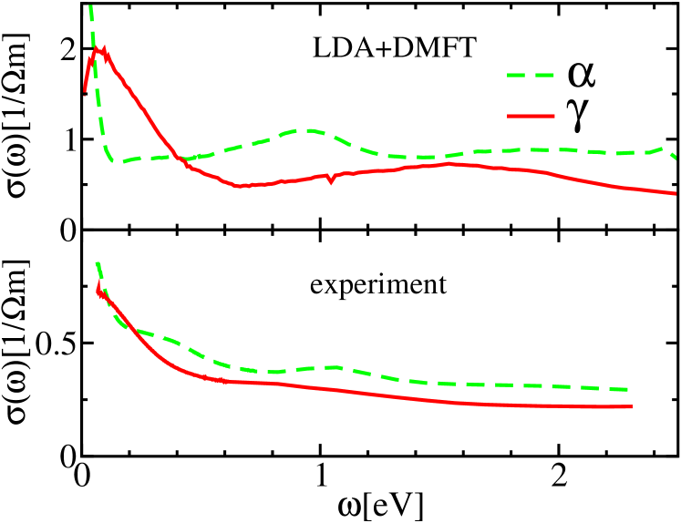
Figure 2: The top panel shows the optical conductivity calculated by LDA+DMFT method for both $\alpha$ and $\gamma$ phase of Cerium. The volume of $\alpha$ phase is $28.06{\rm\r{A}}^{3}$ and the temperature used in calculation is $580K$. The volume of $\gamma$ phase is $34.37{\rm\r{A}}^{3}$ and $T=1160K$. The bottom panel shows experimental results measured by the group of D. van der Marel VanDerMarel . The measurements for $\alpha$ phase were done at 5 K and for $\gamma$ phase at 300 K.

Results - What distinguishes the $\alpha$ phase from the $\gamma$ phase when looking at the optical response of Cerium? How do the calculated results compare with experiments? In the top panel of Fig. 2 we present the calculation of LDA+DMFT method while in the bottom panel the results of experiment on thin films VanDerMarel are reproduced. Notice that in both the experiment and theory the overall magnitude of conductivity in $\gamma$ phase is smaller than in $\alpha$ due to the larger volume and hence reduced velocity of $\gamma$ phase. In the $\alpha$ phase, the Drude peak width is of the order of $0.1$ eV while in $\gamma$ phase it is at least an order of magnitude narrower. This provides us with a crude estimate of $T_{K}$, which is of the order of $1000$ K and $100$ K in the $\alpha$ and $\gamma$ phase, respectively. The intermediate frequency range in $\alpha$ is characterized by a dip or pseudogap ranging from $0.2$ eV to $0.8$ eV and a peak around $1$ eV. This gap is filled–in in $\gamma$ phase resulting in a broad hump up to $0.5$ eV. This nontrivial behavior can be understood by examining the orbitally resolved partial density of states displayed in Fig. 3.

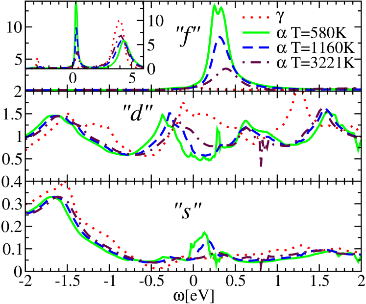
Figure 3: Temperature dependence of partial density of states for both phases $\alpha$ and $\gamma$ of Ce.

The largest contribution to the total density of states around the Fermi level comes from the $f$ bands which have much smaller velocities and, at the same time, almost all spectral weight above the Fermi level. Hence, the transitions from below to above the Fermi level have a small amplitude therefore $f$ bands make a very small contribution to the optical response. Indeed, we found that the contribution involving only $f$ electrons is orders of magnitude smaller than contribution of the $d$ bands. Since $s$ and especially $p$ bands have very little spectral weight close to the Fermi level, the most important contribution to the optical response comes from the $d$ bands.

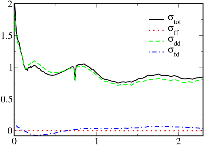
Figure 4: The partial contribution to the optical conductivity of $\alpha$ phase of $Ce$ at $T=1160K$.

To shed some light on the states probed optically we introduce an orbital resolution of the optical conductivity (or ”fat optics”).

$$\sigma(\omega)=\sigma^{ff}(\omega)+\sigma^{dd}(\omega)+\sigma^{fd}(\omega)$$ (6)

where $ff$ stands for the pure $f$ contribution, $dd$ for pure $spd$ contribution and $fd$ for the mixed part. The partial conductivities are calculated by taking the appropriate dipole matrix elements $M_{{\mathbf{k}}jj^{\prime}}$ in Eq. (4), for example, to calculate $ff$ part all four indexes $\alpha_{1},\alpha_{2},\alpha_{3},\alpha_{4}$ in Eq. (5) run over $f$ orbitals only while in $dd$ part all indexes run over $spd$ orbitals. The results displayed in Fig. 4, demonstrate that indeed the optical conductivity has very little $f$ character.

The small contribution of the $f$ electrons to the optical conductivity, however, does not imply that the large Kondo peak, which has $f$ character, is irrelevant for the optical conductivity. The $f$ electrons, mixing with the $spd$ bands, form a large Kondo peak that increases as the temperature is reduced and eventually induces a hybridization pseudogap in $spd$ spectra. As one can see in Fig. 3, the $d$ bands in $\alpha$ phase have a very pronounced pseudogap which is growing by lowering temperature exactly as the Kondo peak builds up. The spectral weight is transferred from the Fermi level into the side–peaks which are $1$ eV apart causing $1$ eV peak in optical conductivity. In the $\gamma$ phase, the Kondo peak disappears because the effective hybridization of the $f$ with $spd$ electrons is smaller and Kondo scale $T_{K}$ is reduced for at least an order of magnitude. In this regime the hybridization pseudogap in the $d$ bands is not formed, and instead we find a broad hump in the optical response.

Although all basic features of measured optical response are well explained by LDA+DMFT calculation, there are some discrepancies. The overall magnitude of measured conductivity in both phases is approximately half of the calculated value. This discrepancy might be a consequence of negligence of interactions on the $spd$ electrons, an effect which would reduce the current matrix elements. Early measurements by Rhee. et.al. Rhee , hovewer, suggest that the optical conductivity is indeed for factor of two larger than the one measured by the group of D. van der Marel VanDerMarel . Also the shoulder in $\alpha$ phase, appearing around $0.33$ eV in Fig. 2b, is absent in LDA+DMFT results.

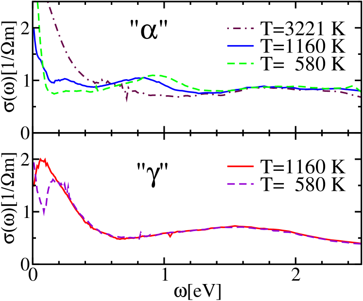
Figure 5: Temperature dependence of optical conductivity for both phases $\alpha$ and $\gamma$ of Ce.

The temperature dependence of the optical response for both the $\alpha$ and $\gamma$ phase are shown in Fig. 5. With increasing temperature, the $1$ eV peak moves to smaller frequencies and finally at few $1000$ K disappears. At the same time, the pseudogap below the peak gradually disappears as the temperature is raised and evolves into a broad hump, just like the one in $\gamma$ phase. This temperature dependence is easily understood by looking at the partial density of states in Fig. 3. Since the Kondo peak is gradually reduced with increasing temperature the hybridization pseudogap in $d$ bands disappears causing featureless optical response. In $\gamma$ phase, the Kondo peak is very small and causes some temperature dependence at very low temperatures only at very low frequency below $0.1$ eV.

Conclusion - The methodology we introduced, allow us to interpret the optical spectra of $\alpha$ and $\gamma$ Cerium, in favor of the Kondo volume collapse model. The formalism should be useful in many other problems of correlated electrons where temperature dependent transfer of spectral weight between widely different energy ranges takes place, a phenomena which can be beyond the scope of simple model Hamiltonians.

References

- (1) B. Johansson, Philos. Mag. 30, 469 (1974).
- (2) J.W. Allen and R.M. Martin, Phys. Rev. Lett. 49, 1106 (1982); J.W. Allen and L.Z. Liu, Phys. Rev. B 46, 5047 (1992).
- (3) For recent reviews see K. Held et al., Psi-k Newsletter #56 (April 2003), p. 65; A. I. Lichtenstein, M. I. Katsnelson, and G. Kotliar,in Electron Correlations and Materials Properties 2, ed. A. Gonis (Kluwer, NY)[cond-mat/0211076].
- (4) M.B. Zölfl, I.A. Nekrasov , Th. Pruschke, V.I. Anisimov, and J. Keller, Phys. Rev. Lett 87, 276403 (2001).
- (5) K. Held, A.K. McMahan, and R.T. Scalettar, Phys. Rev. Lett. 87, 276404 (2001); A.K. McMahan, K. Held, and R.T. Scalettar, Phys. Rev. B 67, 075108 (2003).
- (6) D.M. Wieliczka, C.G. Olson, and D.W. Lynch, Phys. Rev. Lett. 52, 2180 (1984); E. Weschke, C. Laubschat, T. Simmons, M. Domke, O. Strebel, and G. Kaindl, Phys. Rev. B 44, 8304 (1991); F. Patthey, B. Delley, W.D. Schneider, and Y. Baer, Phys. Rev. Lett. 55, 1518 (1985).
- (7) J.W. van der Eb, A. B. Kuz’menko, and D. van der Marel, Phys. Rev. Lett. 86, 3407 (2001).
- (8) J.Y. Rhee, X. Wang, B.N. Harmon, and D.W. Lynch, Phys. Rev. B 51, 17390 (1995).
- (9) Th. Pruschke and N. Grewe, Z. Phys. B: Condens. Matter 74, 439, 1989.
- (10) K. Haule, S. Kirchner, J. Kroha, and P. Wölfle, Phys. Rev. B 64, 155111, (2001).
- (11) Ph. Lambin and J.P. Vigneron, Phys. Rev. B 29, 3430, (1984).
- (12) A.K. McMahan, C. Huscroft, R.T. Scalettar, and E.L. Pollock, J. Comput.-Aided Mater. Des. 5, 131 (1998).