Vortex configurations and metastability in mesoscopic superconductors

Abstract

The vortex dynamics in mesoscopic superconducting cylinders with rectangular cross section under an axially applied magnetic field is investigated in the multivortex London regime. The rectangles considered range from a square up to an infinite slab. The flux distribution and total flux carried by a vortex placed in an arbitrary position of the sample is calculated analytically by assuming Clem’s solution for the vortex core. The Bean-Livingston energy barrier is also analytically calculated in this framework. A Langevin algorithm simulates the flux penetration and dynamical evolution of the vortices as the external field is slowly cycled. The simulated magnetization process is governed by metastable states. The magnetization curves are hysteretic, with paramagnetic response in part of the downward branch, and present a series of peaks corresponding to the entry or expulsion of a single vortex. For elongated rectangles, the vortices arrange themselves into parallel vortex chains and an additional modulation of the magnetization, corresponding to creation or destruction of a vortex chain, comes out.

Key words: Vortex patterns, surface barrier, mesoscopic, vortex dynamics

1 Introduction

Since the pioneering work of Abrikosov [1], it is well known that in a macroscopic type-II superconductor the magnetic field, in the so-called mixed state, penetrates in the form of singly quantized flux lines (or vortices), which form a triangular lattice. For finite samples the vortices are formed at the surface and then pulled to the sample center by the shielding Meissner currents. Notwithstanding, close to the sample edge, a vortex is strongly attracted by the superconductor- vacuum interface. These competing interactions give rise to a energy barrier, the so-called Bean-Livingston surface barrier, which retards the movement of vortices towards the sample center [2, 3]. In samples with very smooth interfaces, this barrier leads to irreversible field-dependent magnetization loops $M(H)$ and finite critical currents even in the absence of inhomogeneities [4, 5]. Nevertheless, defects in the interface may cause the local destruction of the surface barrier, opening leaks for vortex entry.

Recent progress in nanostructuring of superconducting materials [6, 7] has provided the opportunity of studying the vortex state in mesoscopic samples, i.e. whose dimensions are of the order of the penetration depth $\lambda$ and/or the coherence length $\xi$, with sharp interfaces and no noticeable pinning. At these length scales the vortex lattice and the vortex itself may present new and very interesting properties, as for example, the formation of multi-quanta giant vortices, vortex molecules and chain-like vortex arrangements. These vortex structures are strongly dependent on the sample geometry and size, as has been shown by numerical and analytical solutions of the Ginzburg-Landau (GL) equations [9, 10] and experiments [6, 10], and may appear even in samples made of type-I materials (with $\kappa=\lambda/\xi<1/\sqrt{2}$), such as aluminium. The reason is that in thin films the parameter governing the appearance of vortices is actually the effective GL parameter, $\tilde{\kappa}=\Lambda/\xi$, where $\Lambda=\lambda^{2}/d$ may be much greater than $\lambda$ for small sample thicknesses $d$. The choice between the multivortex and the giant vortex states depends on the value of $\tilde{\kappa}$ [8] and on the system size as well. Here we shall consider only systems with high $\kappa$ and sizes comparable to $\lambda$, though larger than $\xi$. For these systems the multivortex state persists over a wide area of the phase diagram.

In the course of our recent research with mesoscopic superconductors [14, 15, 16] we have been studying the vortex dynamics, within the London approximation, in films, multilayers, and strips, submitted to an external magnetic field and dc currents. In this article we present new results for mesoscopic rectangles in the presence of an applied magnetic field. The vortex structure and the energy surface barrier present in these systems are described within the London limit of the Ginzburg-Landau equations. The magnetization process is simulated by a fast algorithm based on Langevin dynamics. We observe, for elongated rectangles, the appearance of vortex chain states and transitions between these states resulting in a modulation of the magnetization loop. Particular attention is given to the formation of metastable vortex configurations in these systems during the magnetization process, which leads to hysteretic magnetization curves with paramagnetic response in part of the downward branch.

2 Vortex structure and the Bean-Livingston barrier

In the high-$\kappa$ limit, the superconducting order parameter is essentially homogeneous except near a vortex core, where its spatial distribution may be given approximately by [11]

$$\psi(\rho)\approx\frac{\rho e^{i\varphi}}{(\rho^{2}+2\xi^{2})^{1/2}}\,,$$ (1)

where $\rho$ is the distance to the vortex center. For points ${\bf r}=(x,y)$ far away from the vortex core, located at ${\bf r}^{\prime}=(x^{\prime},y^{\prime})$, $|\psi({\bf r})|$ is uniform and the second Ginzburg-Landau (GL) equation reduces to the London equation ,

$$-\lambda^{2}\nabla^{2}b(x,y)+b(x,y)=\phi_{0}\delta({\bf r-r^{\prime}})\,.$$ (2)

The solution near the vortex core may be accomplished very precisely by inserting the variational trial function (1) into the GL free energy functional. The result is equivalent to making the cutoff $b(r)\rightarrow b(\sqrt{r^{2}+2\xi^{2}})$ in the London solution for the vortex local induction.

In this spirit, one may compute the flux distribution of a vortex confined in a cylinder if the appropriate boundary condition is used. Here we consider long cylinders with a rectangular cross section of width $W$ and length $L$. An external magnetic field $H$ is applied axially and the vortices are assumed to be perfectly aligned with ${\bf H}$. This problem has been considered previously within the London theory by Sardella, Doria and Netto [12]. Here we shall use Clem’s variational solution for the vortex core to compute the local field distribution and the position-dependent, effective flux carried by a vortex. The result for the local induction generated by a vortex is

$$b_{v}(x,y) = \frac{\phi_{0}}{\lambda W}\sum^{\infty}_{m=1}\frac{\cos k_{m}x_{-}-\cos k_{m}x_{+}}{k_{m}}\times$$

$$\frac{\cosh k_{m}(L-y_{-})-\cosh k_{m}(L-y_{+})}{\sin k_{m}L}$$

where $k_{m}=m\pi/W$, $\alpha_{+}=\alpha+\alpha^{\prime}$ and $\alpha_{-}=|\alpha-\alpha^{\prime}|+\xi$ ($\alpha=x,y$). With this solution, one can compute the interaction energy between vortex $i$ and $j$ in the usual way, that is, $E_{vv}(x_{i},y_{i};x_{j},y_{j})=\phi_{0}b_{v}^{(j)}(x_{i},y_{i})$. Integrating the local induction $b_{v}(x,y)$ over the entire sample area, one finds the effective magnetic flux carried by a vortex,

$$\phi(x,y) = \phi_{0}\Big{[}1-\frac{\cosh(x/\lambda-W/2\lambda)}{\cosh W/2\lambda}-\frac{4}{\lambda^{2}W}\times$$ (4)

$${\sum_{m=1}^{\infty}}^{\prime}\frac{\sin k_{m}x}{k_{m}^{3}}\frac{\cosh k_{m}(y-\frac{L}{2})}{\cosh k_{m}L/2}\Big{]}\,.$$

The prime in the sum operator indicates that only the terms where $m$ is odd are taken into account. Note that in mesoscopic samples the effective flux may be quite smaller than the flux quantum, even for a vortex positioned at the sample center, where $\phi(x,y)$ is maximum.

The homogeneous solution of Eq. 2 corresponds to the local Meissner screening flux distribution, which is given by

$$b_{M}(x,y) = H\Big{[}\frac{\cosh(x/\lambda-W/2\lambda)}{\cosh W/2\lambda}+\frac{4}{\lambda^{2}W}\times$$ (5)

$${\sum_{m=1}^{\infty}}^{\prime}\frac{\sin k_{m}x}{k_{m}^{3}}\frac{\cosh k_{m}(y-\frac{L}{2})}{\cosh k_{m}L/2}\Big{]}$$

$$= H\Big{[}1-\frac{\phi(x,y)}{\phi_{0}}\Big{]}\,.$$

This field distribution is minimum at the samples center. Thus, the Meissner screening current density, ${\bf j}_{M}=\mu_{0}^{-1}\nabla\times{\bf b}_{M}$, repels the vortex away from the surfaces, towards the sample center. The corresponding potential energy felt by the vortex is then given by $E_{M}=\phi_{0}b_{M}(x^{\prime},y^{\prime})$.

On the other hand, there is an energy cost to put a vortex inside the superconducting specimen. This is given by the vortex self-energy

$$E_{self}=\frac{1}{2}E_{vv}({\bf r=r}^{\prime}).$$ (6)

This energy depends on the vortex position and is maximum at the sample center. That is, the vortex is attracted by the surfaces or, in other words, by its images, which are necessary to satisfy the boundary conditions. The attractive self-energy and the repulsive Meissner energy form the well known surface (Bean-Livingston) barrier, which delays vortex entrance and exit in the superconducting sample.

In Fig. 1, we make a surface plot of the energy distribution in a superconducting rectangle with $W=0.2\lambda=20\xi$ and $L=2W$ for three different situations. In Fig. 1(a), H equals the lower critical field, $H=H_{c1}$, for which there is a global minimum at the sample center and a strong energy barrier near the sample surfaces. In mesoscopic samples the activation energy to overcome this barrier is usually much higher than the thermal energy $k_{B}T$. In Fig. 1(b), $H=H_{en}$, where the surface barrier for the first vortex entry disappears. The entrance field may be defined as $\partial{E}_{self}/\partial{x}=-\partial{E}_{M}(H_{en})/\partial{x}$, with the derivatives being evaluated at one of the points $(x,y)=(\xi,L/2)$ or $(D-\xi,L/2)$, as suggested by Fig. 1(b). Note that in the smaller edges of the sample, the barrier is still present, which means that in a rectangle the first vortex tends to enter the sample through one of the larger edges. The total energy when a vortex is placed at the sample center at $H=H_{en}$ is depicted in Fig. 1(c). In this case, a new energy barrier for the entrance of a second vortex is developed. This means that, at zero temperature, the second vortex will be allowed to enter the sample only at a field $H_{2}>H_{en}$. In the field region $H_{en}\leq H<H_{2}$, the sample behaves as in the Meissner state.

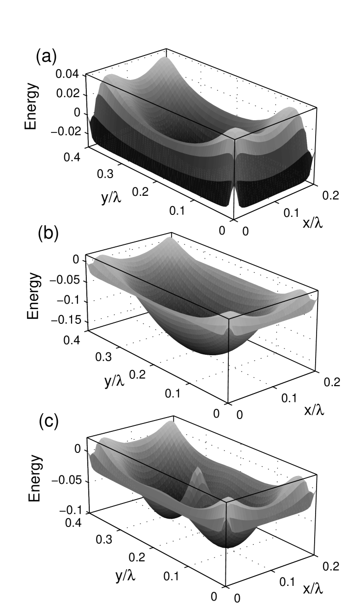
Figure 1: (a) and (b): Energy distribution in a superconducting rectangle with $W=0.2\lambda=20\xi$ and $L=2W$ in the absence of vortices at the first critical field, $H=H_{c1}$ (a), and at the entrance field, $H=H_{en}$ (b). (c) The total energy when a vortex is located at the sample center at $H=H_{en}$.

3 Langevin dynamics and simulation scheme

Next, we review our model to study vortex dynamics in confined geometries. The time evolution of a vortex is described by overdamped Langevin equations of motion,

$$\eta{\bf v}_{i}=-\nabla_{i}E+\mbox{\boldmath$\Gamma$}_{i}(t)\,,$$ (7)

where

$$E = \frac{1}{2}\sum_{i,j}E_{vv}({\bf r}_{i},{\bf r}_{j})+$$ (8)

$$\sum_{i}\big{[}E_{self}({\bf r}_{i})+E_{M}({\bf r}_{i})\big{]}$$

is the total energy of the vortex distribution, $\eta$ is the Bardeen-Stephen friction coefficient, ${\bf v}_{i}$ is the vortex $i$ velocity. $\mbox{\boldmath$\Gamma$}_{i}$ is a Gaussian stochastic noise related with a small temperature $T$ and the friction $\eta$ by $\langle\Gamma_{\alpha,i}(t)\Gamma_{\beta,j}(t^{\prime})\rangle=2\eta k_{B}T\delta_{\alpha\beta}\delta_{ij}\delta(t-t^{\prime})$, where the Greek indices stand for the directions $x$ or $y$. This temperature plays the role of accelerating the convergence towards a stationary state.

The simulation consists in numerically integrating the coupled Langevin equations for all vortices inside the sample. The integration is based on a finite difference algorithm. A vortex is allowed to enter the sample and participate on the dynamics if it satisfies a force balance condition near one of the sample surfaces. The procedure is the same adopted in earlier publications [14, 15, 16]: at each time step a test vortex is placed in a random position a distance $\xi$ from one of the sample interfaces and the total force acting on it is calculated. If this force points to the sample interior, the vortex is accepted, otherwise it is rejected.

The magnetization loops are calculated as an external field is varied in small steps during up to $5\times 10^{5}$ time steps. We verified that the time between successive field changes is large enough for the system to relax to the desired stationary states. The magnetization $M=\mu_{0}^{-1}B-H$ is calculated by integrating the total amount of magnetic induction $B$ inside the sample, $B=\frac{1}{WL}\big{[}\int\!dx\,dy\,b_{M}(x,y)+\sum_{i}\phi(x_{i},y_{i})\big{]}$.

4 Vortex chain states in mesoscopic films

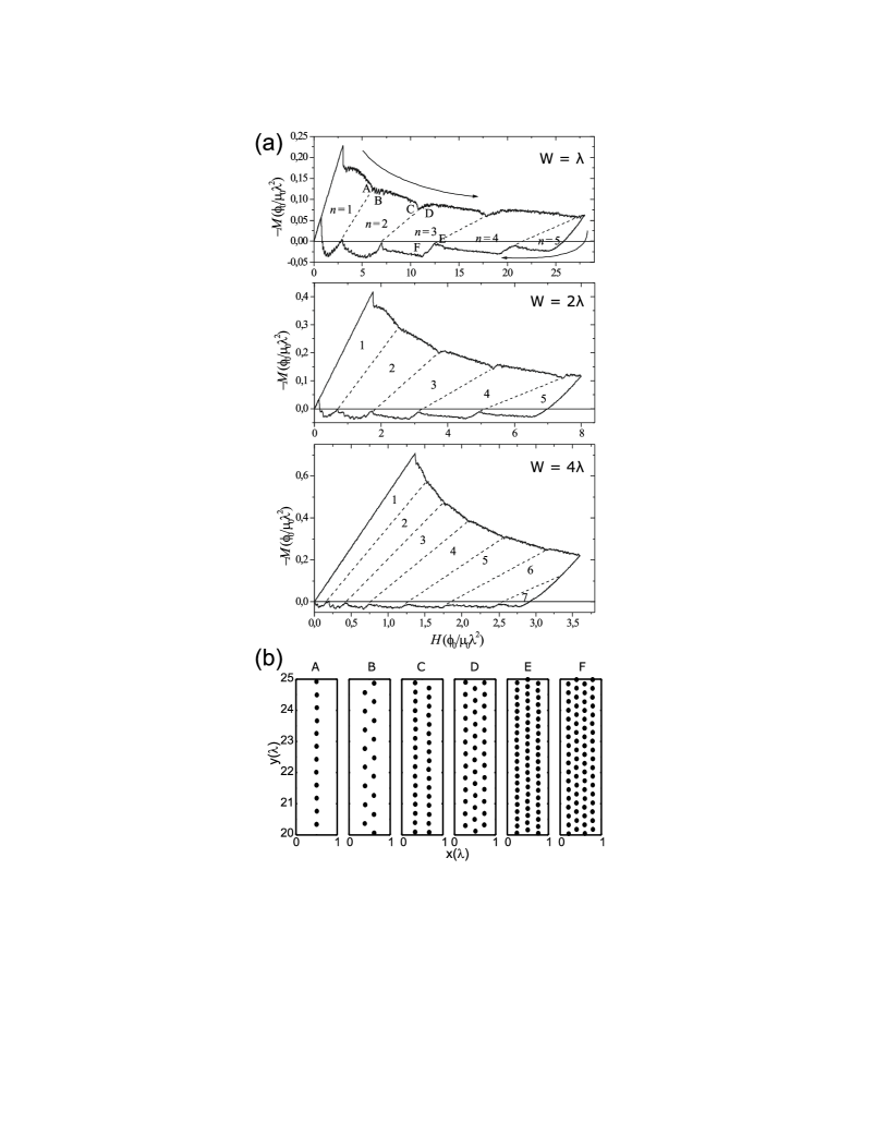
Figure 2: (a) Field dependent magnetization loops for infinite films of width $W=\lambda$, $2\lambda$ and $4\lambda$. The dashed lines are just guides for a better identification of the transitions between successive vortex chain states. (b) Snapshots of the vortex lattice in the points of the magnetization loop indicated at the $W=\lambda$ film magnetization curve.

Here, we consider the case where $L\rightarrow\infty$, which corresponds to a film infinitely long in the $y$ and $z$ directions. To perform the simulation, we take a slice $L_{y}$ in the $y$ direction and assume periodic boundary conditions at $y=0,L_{y}$, in such a way that the simulation is restricted to the region $0\leq x\leq W$, $0\leq y\leq L_{y}$.

In Fig. 2(a) we show magnetization loops for several film thicknesses, $W/\lambda$ = 1, 2 and 4. We choose $\kappa=20$ and $L_{y}=40\lambda$. All the loops are characterized by hysteretic behavior and a distribution of peaks at specific field values. Snapshots of the vortex configurations [some of which are depicted in Fig. 2(b)] show that the VL is composed of $n$ linear chains of vortices parallel to the film surfaces and the extra magnetization peaks are associated with sudden rearrangements of the VL to accommodate a new vortex chain ($n\rightarrow n+1$ transitions), in the case of increasing magnetic field, or destroy an existent chain ($n\rightarrow n-1$ transitions), for decreasing field. Note that as the film thickness increases the matching peaks become less evident in the magnetization loops, that is, the film gradually crosses over from mesoscopic to macroscopic behavior. The matching effect of vortex chains in thin slabs ($W<\lambda$) has been studied in the framework of thermodynamic equilibrium[13]. Our approach assumes that a vortex nucleates at the surfaces, i.e., for fields just above $H_{c1}$ it has to overcome a strong energy barrier in order to find the global minimum at the equatorial plane of the film. Hence we are dealing with steady metastable states. This situation is closer to real experimental conditions, where the time necessary for the system to relax to the thermodynamic equilibrium is not accessible. In this case the critical fields where the transitions $n\rightarrow n\pm 1$ take place are history dependent. In Fig. 2(b) we show snapshots of the vortex configuration in a slice of the $W=\lambda$ film for different points of the magnetization cycle indicated in the upper panel of Fig. 2(a).

5 Vortex states in mesoscopic rectangles

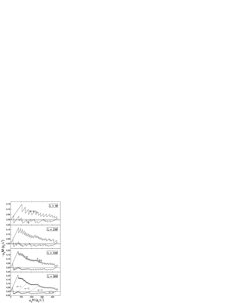
Figure 3: (a) Magnetization loops of rectangles of different aspect ratio, $W/L$ = 1/1, 1/2, 1/4, and 1/8, with $W=0.2\lambda=20\xi$.

Now we consider the more general case of long cylinders with rectangular cross section. The calculations were performed for different aspect ratios, $W/L$ = 1/1, 1/2, 1/4, and 1/8, with $W$ fixed at $W=0.2\lambda$ and $\kappa=100$. The magnetization loops for these samples are depicted in Fig. 3 and in Fig. 4 we show some vortex configurations for the $L=W$ and $L=4W$ samples. The magnetization peaks correspond to entry (in the upward magnetization branch) or expulsion (in the downward branch) of an individual vortex. In some points of the magnetization curve of the longer samples ($L=4W$ and $L=8W$), jumps of two or more vortices are also observed, specially at higher fields.

States with same vorticity may have two distinct metastable solutions, depending on whether the field is going up or down. This is illustrated in Figs. 4(c) and (d), where in the state with vorticity five in a square, vortices arrange in a pentagon, in upward field, or in a face centered square, in downward field.

As the rectangle is elongated the vortices organize into parallel chains of vortices resembling the chain states in infinite films. The effect of these arrangements are seen as a modulation of the magnetization loop. Note that the magnetization curve of the $L=8W$ rectangle is particularly similar to that of the magnetization of the $W=\lambda$ infinite film. In both systems the ratio $W/\xi=20$.

Figure 4: Vortex configurations in a square (a-d) and for a rectangle with $L=8W$ (e-g), both considering $W=0.2\lambda=20\xi$. The points in the magnetization curve corresponding to these configurations are indicated in Fig. 3

As illustrated in Figs. 2 and 3, hysteresis in the magnetization curve is a property shared by all the samples studied here and is a result of the different circumstances in which vortices enter or are expelled from the sample through the surface barrier. The surface barrier delays the incursion of vortices towards the sample interior. As a result, in increasing magnetic field, the vortex lattice is driven into successive superheated metastable states and the diamagnetic response is stronger than the expected for the thermodynamic equilibrium. In decreasing field, a surface barrier is also present, now against vortex expulsion. In this case the system is driven into supercooled metastable states and the response is paramagnetic in most part of the downward branch of the magnetization loop. It is interesting to note that this behavior of the magnetic response, diamagnetic in upward field and paramagnetic in part of the downward branch, is quite frequent in superconducting mesoscopic samples of different geometries and in a broad range of $\kappa$ values [17, 8, 18]. It has been shown that this may be explained in terms of flux capture due to the sample boundaries [18]. Here, Figs. 2 and 3 suggest that this effect may persist even for macroscopic homogeneous samples.

6 Conclusions

In conclusion, we have presented a theoretical study of the surface barrier in mesoscopic superconducting samples and its effect on the formation of metastable vortex structures. Using a Langevin dynamics simulation, magnetization loops of mesoscopic rectangles of several aspect ratios were calculated. All these loops are hysteretic and present series of magnetization jumps due to penetration or expulsion of a vortex. An additional modulation of the magnetization curve is caused by the formation of vortex chain states in the more elongated rectangles. Due to the surface barrier, the vortex configurations are metastable in both branches of the magnetization loop. The capture of vortices in the downward branch leads to paramagnetic response, even for the largest samples studied.

References

- [1] A. A. Abrikosov, Zh. Eksp, Teor. Fiz. 32 (1957) 1442 [Soviet Phys. - JEPT 5 (1957) 1774].
- [2] C. P. Bean, and J. D. Linvsgton, Phys. Rev. Lett. 12 (1964) 14.
- [3] P. G. de Gennes, Superconductivity of Metals and Alloys (Benjamin, New York, 1966), p. 76.
- [4] J. R. Clem, in Low Temperature Physics, edited by K. D. Timmerhaus, W. J. O’Sullivan, and E.F. Hammel (Plenum, New York, 1974) vol. 3 p.102.
- [5] L. Burlachkov, Phys. Rev. B 47 (1993) 8056
- [6] A.K. Geim, I.V. Grigorieva, S.V. Dubonos, J.G.S. Lok, J.C. Maan, A. E. Filippov, F.M.Peeters, Nature (London) 390 (1997) 259.
- [7] V.V. Moshchalkov, V. Bruyndoncx, L. Van Look, M.J. Van Bael, Y. Bruynseraede, and T. Tomomura, Handbook of Nanostructured Materials and Nanotechnology, Vol.3, H.S. Nalwa ed. (Academic Press, 2000).
- [8] V.A. Schweigert, F.M. Peeters, P.S. Deo, Phy. Rev. Lett. 81 (1998) 2783.
- [9] V.A. Schweigert, F.M. Peeters, Phy. Rev. Lett. 83 (1999) 2409; ibid., Physica C 332 (2000) 12.
- [10] L.F. Chibotaru, A. Ceulemans, V. Bruyndoncx, and V.V. Moshchalkov, Nature (London) 408, 833 (2000); ibid. Phys. Rev. Lett. 86 (2000) 1323.
- [11] J.R. Clem, J. Low Temp. Phys. 18 (1975) 427; C. Hu, R.S. Thompson, Phys. Rev. B 6 (1972) 110.
- [12] E. Sardella, M. M. Doria and P.R.S. Netto, Phys. Rev. B 60 (2000) 13158.
- [13] S.H. Brongersma, E. Verweij, N.J. Koeman, D.G. de Groot, R. Griessen, and B. I. Ivlev, Phys. Rev. Lett. 71 (1993) 2319; G. Carneiro, Phys. Rev. B 57 (1998) 6077.
- [14] C.C. de Souza Silva, L.R.E.Cabral, J.A. Aguiar, Phys. Rev. B 63 (2001) 134526; C.C. de Souza Silva, J.A. Aguiar, Physica C 354 (2001) 232-236.
- [15] C.C. de Souza Silva, L.R.E. Cabral, J.A. Aguiar, Physica C, 369 (2002) 217-221.
- [16] C.C. de Souza Silva, J. A. Aguiar, Physica C 388-389 (2003) 673-674.
- [17] A.K. Geim, S.V. Dubonos, J.G.S. Lok, M. Henini, J.C. Maan, Nature (London) 390 (1997) 259.
- [18] V.V. Moshchalkov, X.G. Qui, V. Bruyndoncz, Phys. Rev. B 55 (1997) 11793.