Isotropic-Nematic Transition in Liquid-Crystalline Elastomers:
Lattice Model with Quenched Disorder

Abstract

When liquid-crystalline elastomers pass through the isotropic-nematic transition, the orientational order parameter and the elastic strain vary rapidly but smoothly, without the expected first-order discontinuity. This broadening of the phase transition is an important issue for applications of liquid-crystalline elastomers as actuators or artificial muscles. To understand this behavior, we develop a lattice model of liquid-crystalline elastomers, with local directors coupled to a global strain variable. In this model, we can consider either random-bond disorder (representing chemical heterogeneity) or random-field disorder (representing heterogeneous local stresses). Monte Carlo simulations show that both types of disorder cause the first-order isotropic-nematic transition to broaden into a smooth crossover, consistent with the experiments. For random-field disorder, the smooth crossover into an ordered state can be attributed to the long-range elastic interaction.

I Introduction

Liquid-crystalline elastomers are complex materials consisting of crosslinked polymer networks covalently bonded to long, rigid, liquid-crystalline units warner96 ; terentjev99 ; warner03 . Because of this unusual structure, they combine the elastic properties of rubbers with the anisotropy of liquid crystals. Any distortion of the polymer network affects the orientational order of the liquid crystal, and, likewise, any change in the magnitude or direction of the orientational order influences the shape of the elastomer. These materials have a low-temperature nematic phase, with long-range orientational order in the liquid-crystalline units, and a high-temperature isotropic phase, with no long-range orientational order. Near the isotropic-nematic transition, a small change in temperature induces a large change in the orientational order, which causes the elastomer to extend or contract substantially. This thermally induced extension and contraction enables liquid-crystalline elastomers to be used as actuators or artificial muscles thomsen01 ; shenoy02 ; naciri03 .

A key issue for basic and applied research on liquid-crystalline elastomers is understanding the isotropic-nematic transition. In conventional liquid crystals of small molecules, this is a first-order transition, with a discontinuity in the magnitude of the orientational order as a function of temperature. By contrast, experiments on liquid-crystalline elastomers show that both the orientational order and parameter and the elastic strain vary rapidly but smoothly across this transition, with no first-order discontinuity thomsen01 ; shenoy02 ; naciri03 ; schatzle89 ; kaufhold91 ; disch94 ; clarke01 . Apparently the experimental behavior is neither a first- nor a second-order transition, but rather a nonsingular crossover between the isotropic and nematic phases. Although the transition is sharp enough for applications, it is puzzling from the theoretical point of view. We would like to explain the broadening of this phase transition in liquid-crystalline elastomers, compared with the analogous transition in conventional liquid crystals.

In a previous paper selinger02 , we considered two possible explanations for this broadening. The first possibility is that some aligning stress shifts the transition past a mechanical critical point degennes75 , like a liquid-gas transition at high pressure. This aligning stress might arise from an applied tensile stress on the sample, or from an anisotropic internal stress due to crosslinking an elastomer in the nematic phase. The second possibility is that the transition is broadened by heterogeneity in the elastomer. In particular, we considered heterogeneity in the local isotropic-nematic transition temperature.

To assess these two possible explanations, we measured the elastomer strain as a function of temperature over a range of applied tensile stress. We used elastomer samples crosslinked in the nematic phase, which should have a large anisotropic internal stress imprinted by the crosslinking process, and samples crosslinked in the isotropic phase, which should not have an anisotropic internal stress. By analyzing the experimental data, we found three indications that the broadening of the phase transition is caused by heterogeneity. First, the slope of strain vs. temperature at the transition does not depend sensitively on applied stress, in contrast with the prediction for homogeneous elastomers. Second, the broadening occurs even for samples crosslinked in the isotropic phase. Third, the data for strain vs. temperature could not be fit well by the predictions of Landau theory for homogeneous elastomers, but could be fit much better by the homogeneous theory convolved with a heterogeneous distribution of transition temperatures.

Although our previous study showed the importance of heterogeneity for the isotropic-nematic transition in liquid-crystalline elastomers, this study still leaves two open questions. The first issue is the distribution of local strains. The previous theory considered an average over local regions with different transition temperatures. At any given temperature, these regions have different local nematic order parameters and different local strains. It is not clear how regions with different local strains can fit together. The second issue is the type of heterogeneity. The previous theory considered a distribution of the local transition temperature, which could arise from chemical heterogeneity in an elastomer. This type of heterogeneity would be regarded theoretically as random-bond disorder. It is not the only possible type of heterogeneity. Another possibility is a distribution of local stresses, which could arise from local orientational order in different directions at the time of crosslinking. This possibility would be regarded theoretically as random-field disorder. Several recent papers have considered random-field disorder in liquid-crystalline elastomers fridrikh97 ; yu98 ; fridrikh99 ; yu99 ; uchida00 ; xing03 . These studies have shown that random fields strongly affect mechanical properties and correlation functions in the low-temperature nematic phase. However, they have not made predictions for the effects of random-bond or random-field disorder on the temperature-dependent isotropic-nematic transition.

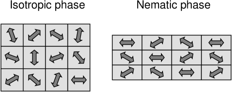
Figure 1: Schematic illustration of the lattice model for the isotropic-nematic transition in liquid-crystalline elastomers. In the isotropic phase, the directors are disordered, and there is no strain. In the nematic phase, the directors are ordered along one axis, and the material is extended with strain along that axis.

The purpose of this paper is to develop a lattice model for liquid-crystalline elastomers, which addresses these theoretical questions about the isotropic-nematic transition. In this model, we explicitly consider both orientational order and elastic strain, as shown in Fig. 1. Orientational order is described by a nematic director, which is defined on each site of a three-dimensional (3D) lattice, as in the Lebwohl-Lasher model of liquid crystals lebwohl72 . By contrast, elastic strain is defined by a single global lattice distortion variable. Because the strain is assumed to be uniform, there is no problem of fitting together regions with different strains. In this model, we can consider either random-bond or random-field disorder. Random-bond disorder enters the model as a variation in the strength of the local coupling constant between local directors on neighboring lattice sites, which implies a variation in the local transition temperature. By comparison, random-field disorder enters the model as a variation in the direction of an aligning field that acts on each local director, which implies a local stress on the elastomer. Both types of disorder are quenched, meaning that they are fixed and cannot evolve toward equilibrium.

Our study leads to four main results. First, we derive a new theoretical formalism for liquid-crystalline elastomers, which translates the Warner-Terentjev neoclassical rubber elasticity warner96 ; terentjev99 ; warner03 into a lattice Hamiltonian for interacting directors and strain. Second, we use Monte Carlo simulations to determine the orientational order parameter and elastic strain of a homogeneous elastomer as a function of temperature and applied stress. These simulations show that the homogeneous elastomer has a mechanical critical point, as expected from Landau theory. Third, we simulate an elastomer with random-bond disorder, and find a broadening of the isotropic-nematic transition in both the orientational order and the strain. This result is consistent with experimental data for liquid-crystalline elastomers. Fourth, we simulate an elastomer with random-field disorder, and find that the transition is also broadened in this case, consistent with experiments, provided that the random field strength is in the right range. The result for the random-field system is surprising, because random fields generally destroy long-range order rather than broadening a transition to an ordered state. We attribute this result to an effective long-range interaction mediated by the elastic strain.

The plan of this paper is as follows. In Sec. II we work out the theoretical formalism, leading to an explicit lattice Hamiltonian that can be simulated. In Sec. III we present the simulations for homogeneous, random-bond, and random-field elastomers, and give numerical results for the isotropic-nematic transition in each case. In Sec. IV we discuss these numerical results, and compare them with experiments and with other theoretical studies of quenched disorder.

II Model

In order to simulate the isotropic-nematic transition in liquid-crystalline elastomers, we need a mathematical model for the interacting orientational and elastic degrees of freedom. In this model, we define a local nematic director $\bm{n}_{i}$ on each site $i$ of a 3D cubic lattice. As in a conventional liquid crystal, the director $\bm{n}_{i}$ is equivalent to $-\bm{n}_{i}$. The directors interact with a global lattice distortion tensor $\bm{\lambda}$, which represents the overall shape of the sample. A schematic view of the directors and lattice distortion is shown in Fig. 1.

The Hamiltonian for this lattice model can be written as

$$F=\sum_{\langle i,j\rangle}F_{\text{interaction}}(\bm{n}_{i},\bm{n}_{j})+\sum_{i}F_{\text{elastic}}(\bm{n}_{i},\bm{\lambda}).$$ (1)

The first term in Eq. (1) is an interaction that favors alignment of the directors on neighboring lattice sites $i$ and $j$. As in the Lebwohl-Lasher model, this interaction can be written explicitly as

$$F_{\text{interaction}}(\bm{n}_{i},\bm{n}_{j})=-J_{ij}(\bm{n}_{i}\cdot\bm{n}_{j})^{2},$$ (2)

where $J_{ij}>0$ is the local bond strength, which may be either uniform or disordered. The second term in Eq. (1) is an elastic term that couples the director orientation at lattice site $i$ with the shape of the polymer chains, which are determined by the overall lattice distortion tensor $\bm{\lambda}$. This term should favor alignment of the directors along an orientation determined by the lattice distortion, and, conversely, favor a lattice distortion in an orientation determined by the directors.

To develop an explicit expression for this elastic term, we use an argument based on the neoclassical rubber elasticity of Warner and Terentjev warner96 ; terentjev99 ; warner03 . In their theory, they derive the general formula

$$F_{\text{elastic}}=\frac{\mu}{2}\left[\text{Tr}\left(\bm{\ell}_{0}\cdot\bm{\lambda}^{T}\cdot\bm{\ell}^{-1}\cdot\bm{\lambda}\right)+\ln\left(\frac{\det\bm{\ell}}{a^{3}}\right)\right],$$ (3)

where $\mu$ is the shear modulus, $\bm{\lambda}$ is the lattice distortion tensor, $\bm{\ell}$ is the shape tensor of the polymer chains, $\bm{\ell}_{0}$ is the shape tensor at the time of crosslinking, and $a$ is the average polymer step length. They further work out a specific expression for the shape tensor in the freely jointed chain model. That specific expression is not appropriate for a lattice Hamiltonian, because it is based on a global average over a system with imperfect nematic order. By contrast, in a lattice model, there is a director on each lattice site, which represents perfect local orientational order along $\bm{n}_{i}$ at site $i$. Any imperfect long-range order must emerge spontaneously from simulations of the interacting system. Hence, we should construct a local shape tensor $\bm{\ell}_{i}$ for site $i$, derived from the director $\bm{n}_{i}$, which will enter into the trace formula of Eq. (3).

To construct the local shape tensor $\bm{\ell}_{i}$, we first consider a coordinate system aligned along the director $\bm{n}_{i}$, in which $\bm{\ell}_{i}$ is diagonal. In that coordinate system, we have

$$\bm{\ell}_{i}^{-1}=\left(\begin{array}[]{ccc}\ell_{\bot}^{-1}&0&0\\ 0&\ell_{\bot}^{-1}&0\\ 0&0&\ell_{\|}^{-1}\end{array}\right),$$ (4)

where $\ell_{\bot}$ and $\ell_{\|}$ are the anisotropic polymer step lengths favored by the local mesogenic unit. In a general coordinate system, the shape tensor components become

$$\ell_{i,\alpha\beta}^{-1}=\ell_{\bot}^{-1}\delta_{\alpha\beta}+\left(\ell_{\|}^{-1}-\ell_{\bot}^{-1}\right)n_{i,\alpha}n_{i,\beta}.$$ (5)

A similar argument gives an explicit expression for the lattice distortion tensor $\bm{\lambda}$. Suppose the lattice is uniformly strained along the axis $\bm{m}$. In a coordinate system aligned with this strain axis, we have

$$\bm{\lambda}=\left(\begin{array}[]{ccc}\lambda^{-1/2}&0&0\\ 0&\lambda^{-1/2}&0\\ 0&0&\lambda\end{array}\right),$$ (6)

where $\lambda$ is the distortion factor, i.e. the strained length normalized by the original length of the sample, which is related to the strain $e$ by $\lambda=1+e$. In a general coordinate system, the distortion tensor components become

$$\lambda_{\alpha\beta}=\lambda^{-1/2}\delta_{\alpha\beta}+\left(\lambda-\lambda^{-1/2}\right)m_{\alpha}m_{\beta}.$$ (7)

The third tensor required for neoclassical rubber elasticity is the shape tensor $\bm{\ell}_{0}$ at the time of crosslinking. For now, suppose the system is crosslinked in a totally disordered state, with no long-range or even local orientational order. In that case, a reasonable model for $\bm{\ell}_{0}^{-1}$ is the isotropic average of $\bm{\ell}^{-1}$. This average gives the tensor components

$$\ell_{0,\alpha\beta}^{-1}=a^{-1}\delta_{\alpha\beta},$$ (8)

where $a^{-1}=(2\ell_{\bot}^{-1}+\ell_{\|}^{-1})/3$.

To determine the elastic term in the lattice Hamiltonian, we substitute the tensor expressions (5), (7), and (8) into the general formula of Eq. (3). In this substitution, we note that $\det\bm{\ell}$ is constant because $\bm{\ell}$ represents perfect local orientational order at a specific lattice site. Hence, the determinant term adds an unimportant constant to the Hamiltonian, and we can neglect it. After some algebra, the trace term leads to

$$F_{\text{elastic}}(\bm{n}_{i},\bm{\lambda})=$$

$$\frac{\mu}{2}\left[\left(\lambda^{2}+2\lambda^{-1}\right)-\gamma\left(\lambda^{2}-\lambda^{-1}\right)\left(\frac{3}{2}\left(\bm{m}\cdot\bm{n}_{i}\right)^{2}-\frac{1}{2}\right)\right].$$

In this expression, the first term is the classical elastic free energy for conventional isotropic elastomers, and the second term represents the anisotropy of liquid-crystalline elastomers. As expected, the second term shows a coupling between the elastic strain and the director orientation. When the lattice is strained, each local director $\bm{n}_{i}$ tends to align along the strain axis $\bm{m}$, with an aligning potential that increases as the distortion $\lambda$ increases above $1$. Conversely, when the directors are aligned, the lattice tends to extend along the average director. The strength of the coupling depends on the parameter

$$\gamma=\frac{2\ell_{\bot}^{-1}-2\ell_{\|}^{-1}}{2\ell_{\bot}^{-1}+\ell_{\|}^{-1}},$$ (10)

which represents the difference in polymer step lengths parallel and perpendicular to the local director. This parameter expresses the anisotropy of the local mesogenic units, and controls how the local director interacts with the strain. It ranges from 0 (in the isotropic case $\ell_{\|}=\ell_{\bot}$) to 1 (in the maximally anisotropic limit $\ell_{\|}\gg\ell_{\bot}$).

We must now consider the possibility of symmetry-breaking fields acting on the elastomer. Symmetry-breaking fields can arise from two possible sources. The simplest possibility is a uniform stress $\sigma$ applied to the elastomer. Such a stress couples to the strain $e$, or equivalently to the distortion $\lambda=1+e$, and gives an additional contribution to the Hamiltonian of $-\sigma\lambda$ for each lattice site. A more subtle possibility is a symmetry-breaking field quenched into the local shape tensor $\bm{\ell}_{0}$ at the time of crosslinking. If the system has long-range order at the time of crosslinking, then $\bm{\ell}_{0}$ is anisotropic with a single principal axis $\bm{n}_{0}$ at all lattice sites. If the system has short-range order at the time of crosslinking, then $\bm{\ell}^{i}_{0}$ is anisotropic with a different principal axis $\bm{n}^{i}_{0}$ at each lattice site $i$.

In principle, we can incorporate the long- or short-range anisotropy of $\bm{\ell}^{i}_{0}$ into the model by writing a general expression for this tensor and substituting it into the trace formula of Eq. (3). The detailed calculation is not algebraically tractable, but by symmetry we can see that the tensor components $\ell^{i}_{0,\alpha\beta}$ must involve a combination of the isotropic tensor $\delta_{\alpha\beta}$ and the anisotropic tensor $n^{i}_{0,\alpha}n^{i}_{0,\beta}$ at site $i$. The anisotropic term acts as an effective field on the director $\bm{n}_{i}$, with a coupling of the form $-(\bm{h}_{i}\cdot\bm{n}_{i})^{2}$. The direction of $\bm{h}_{i}$ is the local quenched-in axis $\bm{n}^{i}_{0}$, and the magnitude of $\bm{h}_{i}$ scales with the magnitude of the local quenched-in nematic order.

By combining Eq. (2), Eq. (II), and the effects of symmetry-breaking fields, we obtain the final expression for the lattice Hamiltonian

$$F = -\sum_{\langle i,j\rangle}J_{ij}(\bm{n}_{i}\cdot\bm{n}_{j})^{2}+\sum_{i}\biggl{[}\frac{\mu}{2}\left(\lambda^{2}+2\lambda^{-1}\right)$$ (11)

$$\ \ \ \ -\frac{\mu\gamma}{2}\left(\lambda^{2}-\lambda^{-1}\right)\left(\frac{3}{2}\left(\bm{m}\cdot\bm{n}_{i}\right)^{2}-\frac{1}{2}\right)$$

$$\ \ \ \ -\sigma\lambda-\left(\bm{h}_{i}\cdot\bm{n}_{i}\right)^{2}\biggr{]}.$$

In this Hamiltonian, the statistical variables are the director $\bm{n}_{i}$ on each lattice site $i$ and the overall lattice distortion $\lambda$. We can assume that the distortion axis $\bm{m}$ is aligned with the principal axis of the director distribution.

This model of Eq. (11) can describe uniform elastomers or elastomers with quenched random-bond or random-field disorder. Uniform elastomers are represented by a bond strength $J_{ij}=J$ independent of position, and by a local field $\bm{h}_{i}=0$. In this case, the system can have an isotropic-nematic transition with a transition temperature $T_{IN}$ that depends on $J$. Random-bond elastomers are represented by a bond strength $J_{ij}$ that depends on the position of the lattice sites $i$ and $j$. We can regard this variation in the bond strength as a variation in the local $T_{IN}$, which could be caused by chemical heterogeneity in the elastomer. Random-field elastomers are represented by a local field $\bm{h}_{i}$ that varies randomly with position. This variation models randomness in the local orientational order at the time of crosslinking, which gives heterogeneous local stresses on the elastomer. We can now perform simulations to study the isotropic-nematic transition in each scenario. These simulations are presented in the following section.

III Simulations

We simulate the model of Eq. (11) using the Monte Carlo method. We run the simulations on a 3D cubic lattice with periodic boundary conditions. We use a 3D rather than a 2D lattice, even though the simulations take longer in 3D, in order to avoid a 2D Kosterlitz-Thouless transition kosterlitz73 . We normally use a lattice of size $36\times 36\times 36$. However, we have run a limited number of simulations on a larger lattice of size $48\times 48\times 48$, for the uniform, random-bond, and random-field cases, and the results are generally consistent. In the simulations, we take the uniform or average value of the bond strength $J_{ij}$ to be 1, and the shear modulus $\mu$ to be 1. These parameters define a scale for the temperature. We let the anisotropy parameter $\gamma$ have its maximum value of 1, in order to see the greatest coupling between orientational order and elastic distortion.

In each Monte Carlo step of the simulations, we attempt one local director rotation per lattice site and one change in the overall elastic distortion $\lambda$. At each temperature, we equilibrate for 3000 Monte Carlo steps, and then collect data for 2000 Monte Carlo steps. This number of steps is sufficient to reach equilibrium at all temperatures except for certain cases of hysteresis, which are discussed below. From the numerical data, we extract two parameters as functions of temperature $T$: the elastic distortion $\lambda(T)$ and the orientational order parameter $S(T)$, which is defined as the largest eigenvalue of the tensor $Q_{\alpha\beta}=\langle\frac{3}{2}n_{i,\alpha}n_{i,\beta}-\frac{1}{2}\delta_{\alpha\beta}\rangle$, averaged over lattice sites $i$. That parameter represents the degree of ordering of the local directors along an average axis.

We begin with the local directors in a disordered configuration, and then cycle the temperature downward and back upward, using the ending configuration at one temperature as the starting point for the next. This temperature cycling mimics the procedure in typical experiments, and provides an explicit test for hysteresis. For most parameter sets, we vary the temperature from 0.9 to 0.8 and back in steps of 0.05, for a total of 41 runs over the temperature range. Each temperature cycle requires approximately 48 hours on a single processor of the Huinalu linux supercluster at the Maui High Performance Computing Center.

Because the temperature cycle gives two runs at each temperature (except the lowest), we can assess whether each run shows a stable, metastable, or unstable state. To test for unstable states, we check whether the order parameter $S$ has stabilized by fitting it as a linear function of the Monte Carlo step number over the final 2000 steps at each temperature. We identify a state as unstable and remove it from our results if the absolute value of the slope exceeds a threshold. In practice, we find that the threshold of $3.2\times 10^{-5}$ eliminates at most two runs from each temperature cycle, one on cooling and one on heating. To test for stability vs. metastability, we compare the values of $S$ for cooling and heating runs at the same temperature. If these values are within six standard deviations of each other, we assume they represent the same stable state, so we average the two runs to obtain one data point with improved statistics. If not, we assume that one state is stable and the other metastable, so we report both in our results.

III.1 Uniform Elastomers

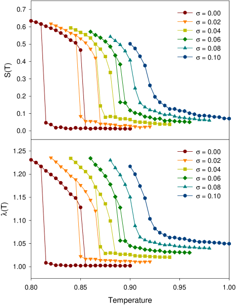
Figure 2: (Color online) Plots of the orientational order parameter $S(T)$ and the elastic distortion $\lambda(T)$ for a homogeneous elastomer under several values of the applied uniform stress $\sigma$. At zero stress, both plots show a first-order isotropic-nematic transition with a large hysteresis. As the stress increases, the first-order discontinuity decreases and then vanishes as the system passes through a mechanical critical point. Temperature is in units of the bond strength $J$.

For an initial series of simulations, we consider uniform elastomers, with no randomness in the bonds (all $J_{ij}=1$) and no random fields (all $\bm{h}_{i}=0$). The numerical results for these simulations are shown in Fig. 2. For zero applied stress $\sigma$, the system has a first-order transition with hysteresis between the high-temperature isotropic phase and the low-temperature nematic phase. On cooling, the orientational order parameter $S(T)$ jumps from 0.05 to 0.62, and the lattice distortion $\lambda(T)$ jumps from 1.01 to 1.22 (1% to 22% strain), at a scaled temperature of 0.81. On heating, $S(T)$ jumps from 0.47 to 0.02, and $\lambda(T)$ jumps from 1.13 to 1.00 (13% to 0% strain), at a scaled temperature of 0.85. The large jumps in both of these order parameters, and the width of the hysteresis region, show the strong first-order character of the transition.

When a symmetry-breaking stress is applied to the uniform elastomer, the phase transition changes drastically. An applied stress increases both order parameters $S(T)$ and $\lambda(T)$ for all temperatures. As the stress becomes larger, the transition temperature increases, the first-order jumps in the order parameters decrease, and the hysteresis region becomes narrower. At a critical value of the stress between 0.06 and 0.08, the first-order jumps vanish and the hysteresis goes away. Beyond that stress, the system shows a smooth supercritical evolution between the high-temperature disordered limit and the low-temperature ordered limit. As the stress continues to increase, this supercritical evolution becomes increasingly broad. This trend with increasing stress is consistent with the prediction of de Gennes based on symmetry considerations degennes75 . It is analogous to the critical point in the liquid-gas transition under high pressure.

The simulations show that the orientational order parameter $S(T)$ and the elastic strain $e(T)=\lambda(T)-1$ have roughly the same dependence on both temperature and applied stress. The linear scaling between $S(T)$ and $e(T)$ is consistent with the prediction based on symmetry considerations.

We note that the smooth evolution of $S(T)$ and $e(T)$ beyond the mechanical critical point agrees with experiments on the isotropic-nematic transition in liquid-crystalline elastomers. However, as discussed in the Introduction, our previous paper found experimental indications that the isotropic-nematic transition is smooth even if an elastomer is not under a supercritical stress selinger02 . For that reason, we need to look for other mechanisms to broaden this transition. Hence, we consider random-bond and random-field disorder in the following sections.

III.2 Random Bonds

Figure 3: Schematic view of the block structure in the simulations with quenched disorder. (a) Random bond strength. (b) Random field orientations.

To simulate disordered systems, we first consider elastomers with variations in the local bond strength. We let the parameters $J_{ij}$ of Eq. (11) be quenched random variables, which are fixed at the beginning of the simulation and do not change in response to the statistical evolution of the directors and the lattice distortion. We suppose that the variation of $J_{ij}$ occurs in blocks, as shown in Fig. 3(a). Within each block, $J_{ij}$ has a uniform value from a Gaussian distribution with mean 1. From block to block, there are no correlations in $J_{ij}$. Both the width of the Gaussian distribution and the size of the blocks are parameters for the model, which are discussed below. Because the isotropic-nematic transition temperature depends on the bond strength, this model represents an elastomer with blocks of different local transition temperature $T_{IN}$. This could occur if the elastomer is chemically heterogeneous, with different compositions in different local regions.

Figure 4: (Color online) Orientational order parameter $S(T)$ for simulations of elastomers with random-bond disorder. (a) Varying magnitude of disorder, with fixed block size $12\times 12\times 12$. (b) Varying block size of disorder, with fixed magnitude $\pm 20\%$. As the disorder magnitude and block size increase, the transition is broadened into a smooth crossover between the isotropic and nematic limits. Temperature is in units of the average bond strength $J_{ij}$.

In Fig. 4(a), we show the results for varying the magnitude of the disorder, i.e. the standard deviation of the Gaussian distribution of $J_{ij}$, for the fixed block size $12\times 12\times 12$. To save space, we show only the plots of the orientational order parameter $S(T)$, because the corresponding plots of the lattice distortion $\lambda(T)$ look quite similar. For weak disorder of $\pm 5\%$, the system has a strong first-order isotropic-nematic transition, which is almost identical to the result for no disorder. Clearly the orientational order can average over this weak disorder strength. For a larger disorder of $\pm 10\%$, there is still a first-order transition, but the first-order discontinuity in $S(T)$ is smaller, and the width of the hysteresis region is greatly reduced. When the disorder reaches $\pm 15\%$, there is no longer a first-order discontinuity nor a hysteresis loop. Instead, the material evolves rapidly but smoothly between the isotropic and nematic limits as a function of temperature. For an even larger disorder of $\pm 20\%$, the transition becomes even broader, with a reduced slope in $S(T)$.

Figure 4(b) presents the results of varying the block size for a fixed disorder magnitude of $\pm 20\%$. For the large block size $12\times 12\times 12$ discussed above, or even for block size $6\times 6\times 6$, the random-bond disorder causes a smooth evolution between the isotropic and nematic states. However, for a reduced block size of $3\times 3\times 3$, there is a first-order isotropic-nematic transition, with a small first-order discontinuity and small hysteresis. If the block size is reduced to $1\times 1\times 1$, i.e. each block is a single lattice site, then the system has a strong first-order transition. Although the disorder strength is quite large, the result for block size $1\times 1\times 1$ is almost identical to the result for no disorder. Hence, reducing the block size is effectively equivalent to reducing the magnitude of disorder. The orientational order can average over small blocks of large disorder, just as it averages over large blocks of small disorder.

The results of this section show that random-bond disorder can change the nature of the isotropic-nematic transition in liquid-crystalline elastomers, provided that the magnitude and length scale of the disorder are sufficiently large. If those conditions are satisfied, then the orientational order parameter $S(T)$ undergoes a continuous change from a low value in the high-temperature isotropic limit to a large value in the low-temperature nematic limit. The lattice distortion $\lambda(T)$ goes through a corresponding smooth evolution. Thus, this type of disorder provides one mechanism to explain the experimental results.

III.3 Random Fields

As an alternative to random bonds, quenched disorder might affect liquid-crystalline elastomers through random fields coupling to the local directors. To simulate random-field effects, we let the fields $\bm{h}_{i}$ of Eq. (11) be quenched random variables, and let the bond strengths $J_{ij}$ be fixed at 1. We suppose that the fields $\bm{h}_{i}$ have a fixed magnitude $h$ and random orientation. As in the random-bond case, we suppose that the randomness occurs in blocks, as shown in Fig. 3(b). The random orientation is uniform at every site within a block, and it has no correlations from block to block. The magnitude $h$ of the random field and the size of the blocks are thus two parameters for this model. Note that this model represents an elastomer with different preferred orientations of the local director in different blocks. This could occur if the crosslinking process quenches heterogeneous local stresses into the polymer network.

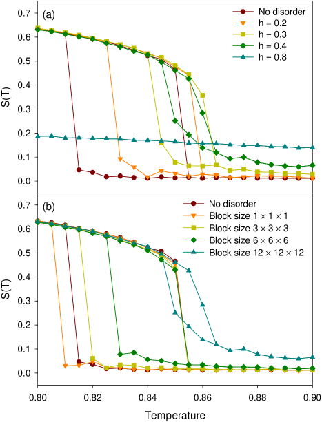
Figure 5: (Color online) Orientational order parameter $S(T)$ for simulations of elastomers with random-field disorder. (a) Varying magnitude of random field, with fixed block size $12\times 12\times 12$. (b) Varying block size, with fixed random-field strength $h=0.4$. As the random-field strength and block size increase, the transition is broadened and then the ordered nematic phase is destroyed. Temperature is in units of the bond strength $J$.

Simulation results for several values of the random-field strength $h$ at fixed block size $12\times 12\times 12$ are presented in Fig. 5(a). For a small random field $h=0.2$, the system has a first-order isotropic-nematic transition, which is fairly close to the result for no disorder. For a slightly larger random field $h=0.3$, the magnitude of the first-order discontinuity and the width of the hysteresis region are both reduced. For $h=0.4$, the first-order transition is much weaker, and the system is close to the smooth crossover between the isotropic and nematic phases seen in the previous two sections. However, for a larger random field $h=0.8$, the behavior is quite different. Instead of broadening the isotropic-nematic transition, the random field simply destroys the long-range nematic order in an athermal way. In that high-field limit, each local director is just aligned with its local random field, giving a slight residual order parameter $S(T)$ that is approximately independent of temperature.

Figure 5(b) shows the simulation results for several values of the block size at the fixed random-field strength $h=0.4$. As in the random-bond case, varying the block size has the same effect as varying the random-field strength. For small block size, the system has a first-order transition that is very close to the result for no disorder. This behavior shows that the orientational order averages over small blocks of strong random field. For larger block size, the phase transition gradually changes toward a smooth crossover between the isotropic and nematic limits. Analogous simulations for $h=0.8$ (not shown) demonstrate that increasing the block size takes the system from a strong first-order transition toward a limit in which orientational order is destroyed for all temperature.

Overall, the simulations presented in this section show that random fields can have two distinct effects on the isotropic-nematic transition in liquid-crystalline elastomers. Low random-field disorder broadens the isotropic-nematic transition, but high random-field disorder destroys the nematic phase in a temperature-independent way. The results for low random-field disorder are consistent with experiments on liquid-crystalline elastomers, but the results for high random-field disorder show a very different type of behavior.

IV Discussion

In this paper, we have investigated three possibile mechanisms to explain the broadening of the isotropic-nematic transition in liquid-crystalline elastomers. The first mechanism is a stress that couples to the strain and hence to the nematic order. Our simulations show that a small stress reduces the first-order discontinuity in the isotropic-nematic transition, and a critical stress causes this discontinuity to vanish. Beyond that point, the elastomer has a smooth crossover between the isotropic and nematic limits as a function of temperature. Hence, a supercritical stress gives the same general trend as the experiments. However, our previous paper found evidence that the smooth isotropic-nematic transition does not require a supercritical stress selinger02 . In particular, a smooth transition is seen even in elastomers crosslinked in the isotropic phase, even under the minimum applied stress required for the experiment, conditions in which a supercritical stress is unlikely to occur.

An alternative possibility to explain the broadened transition is quenched disorder in the elastomer. One specific mechanism to generate quenched disorder is chemical heterogeneity, which can be represented by random bonds in a lattice model. Our simulations show that random-bond disorder can broaden the isotropic-nematic transition into a smooth crossover, if the magnitude and length scale of the disorder are large enough. This numerical result is consistent with theoretical work on generic random-bond systems by Imry and Wortis imry79 , which argued that weak random-bond disorder should reduce the first-order discontinuity in a transition, and larger disorder should eliminate the discontinuity completely. It is also consistent with other simulation studies of the isotropic-nematic transition in systems of small molecules with quenched random impurities dadmun92 ; ilnytskyi99 . Thus, random-bond disorder provides a plausible mechanism to explain experimental results on liquid-crystalline elastomers.

Another type of quenched disorder is heterogeneous local stresses, which can be represented by random fields in a lattice model. In general, random fields have stronger effects on ordered phases and phase transitions than random bonds. In our simulations, we find that low random-field disorder broadens the isotropic-nematic transition, consistent with the experiments, but high random-field disorder destroys the nematic phase over all temperatures.

Our random-field simulation results are surprising in comparison with theoretical expectations for random-field systems. In classic work on quenched disorder, Imry and Ma imry75 showed that arbitrarily small random fields should destroy long-range order in a discrete order parameter (such as an Ising model) for spatial dimension less than 2, and destroy long-range order in a continuous order parameter for spatial dimension less than 4. In our case, the nematic order parameter is continuous, and the spatial dimension is 3. Hence, the Imry-Ma argument implies that random fields should destroy nematic order. The simulations of high random fields show this effect, but the simulations of lower random fields show a broad isotropic-nematic transition, which is a very different effect.

One might ask whether this behavior results from an Imry-Ma domain size that is large compared with the size of the simulation cell. To answer that question, we can estimate the Imry-Ma domain size. In the Imry-Ma argument, domains form with a characteristic size $\xi$ such that the boundary energy equals the field energy. In our 3D system of continuous directors, the boundary energy is of order $J\xi$. To estimate the field energy, recall that we are simulating blocks of sites with the same random field, as shown in Fig. 3. Let $b$ be the linear size of a block. The field energy for a single block is of order $\sum_{\mathrm{block}}{(\bm{h}_{i}\cdot\bm{n}_{i})}^{2}\approx h^{2}b^{3}$, and the number of blocks per domain is of order $(\xi/b)^{3}$. As a result, the field energy for a domain is of order $(h^{2}b^{3})(\xi/b)^{3/2}\approx h^{2}b^{3/2}\xi^{3/2}$. This argument implies that increasing the block size causes the random field to be more effective, as is seen in the simulations. Comparing the boundary energy with the field energy gives an Imry-Ma domain size of $\xi\approx J^{2}/(h^{4}b^{3})$. For the simulated values $J=1$, $h=0.4$, and $b=12$, this size is less than 1 lattice unit, much less than the system size. Thus, the behavior in our simulations does not arise from a large Imry-Ma domain size.

We suggest that the new behavior in our simulations arises from the coupling between the local directors and global elastic strain variable. The Imry-Ma prediction is based on an analysis of the energetics of local ordered domains. This analysis assumes a short-range interaction in the order parameter. By contrast, in our model for liquid-crystalline elastomers, the local director at any lattice site interacts with the global elastic strain, which in turn interacts with the local director at every other lattice site. Hence, the elastic strain mediates an effective long-range interaction between local directors on different sites. This changes the assumptions in the Imry-Ma theory, and hence allows a broad isotropic-nematic transition over a range of random-field strength.

For a specific numerical test of this suggestion, we perform simulations of a simplified model without the globel elastic strain variable. The Hamiltonian for this model consists only of the interaction of Eq. (2) plus the random fields acting on the local directors. In this case, the interaction is purely short-range, so the Imry-Ma argument should apply. Indeed, the simulations show that random fields simply destroy the nematic order and do not induce a broad isotropic-nematic transition. This confirms the concept that a broad transition is a new effect arising from a strain-mediated long-range interaction.

In a realistic system, the elastic strain-mediated interaction is not infinite-range, as in our model. However, elastic interactions do have a power-law form, and hence they can have long-range effects. In a recent renormalization-group study, Xing and Radzihovsky xing03 have assessed the effects of elastic interactions on liquid-crystalline elastomers with random fields. They find that elastic interactions cause the nematic order to be robust against the disordering effect of random fields. Through a power-law expansion about spatial dimensionality 5, they estimate that nematic order can be stable down to a critical dimension well below 3. This is apparently the same stabilization that we see numerically. Thus, our simulation shows the consequence of this stabilization for the temperature-dependent isotropic-nematic transition. It is interesting to note that similar considerations of disorder and long-range elasticity have been seen in models for magnetic phase transitions in colossal magnetoresistance materials burgy04 .

In conclusion, we have developed a lattice model of the isotropic-nematic transition in liquid-crystalline elastomers. The model considers a local directors coupled to a global elastic distortion variable, and allows both random-bond and random-field disorder. Through Monte Carlo simulations of this model, we find that a uniform elastomer has a mechanical critical point, that both random-bond disorder and low random-field disorder broaden the isotropic-nematic transition, and that high random-field disorder destroys the nematic phase. The model therefore confirms that the width of the isotropic-nematic transition can be controlled by heterogeneity in liquid-crystalline elastomers.

- (1) M. Warner and E. M. Terentjev, Prog. Polym. Sci. 21, 853 (1996).
- (2) E. M. Terentjev, J. Phys. Condens. Matter 11, R239 (1999).
- (3) M. Warner and E. M. Terentjev, Liquid Crystal Elastomers (Oxford University Press, Oxford, 2003).
- (4) D. L. Thomsen, P. Keller, J. Naciri, R. Pink, H. Jeon, D. Shenoy, and B. R. Ratna, Macromolecules 34, 5868 (2001).
- (5) D. K. Shenoy, D. L. Thomsen, A. Srinivasan, P. Keller, and B. R. Ratna, Sensors and Actuators A: Physical 96, 184 (2002).
- (6) J. Naciri, A. Srinivasan, H. Jeon, N. Nikolov, P. Keller, and B. R. Ratna, Macromolecules 36, 8499 (2003).
- (7) J. Schätzle, W. Kaufhold, and H. Finkelmann, Makromol. Chem. 190, 3269 (1989).
- (8) W. Kaufhold, H. Finkelmann, and H. R. Brand, Makromol. Chem. 192, 2555 (1991).
- (9) S. Disch, C. Schmidt, and H. Finkelmann, Macromol. Rapid Commun. 15, 303 (1994).
- (10) For an exception, see S. M. Clarke, A. Hotta, A. R. Tajbakhsh, and E. M. Terentjev, Phys. Rev. E 64, 061702 (2001). In this case, the strain seems to increase as a power law below a second-order isotropic-nematic transition. That behavior has not yet been explained theoretically, and we do not address it here.
- (11) J. V. Selinger, H. G. Jeon, and B. R. Ratna, Phys. Rev. Lett. 89, 225701 (2002).
- (12) P. G. de Gennes, C. R. Acad. Sci. Ser. B 281, 101 (1975).
- (13) S. V. Fridrikh and E. M. Terentjev, Phys. Rev. Lett. 79, 4661 (1997).
- (14) Y.-K. Yu, P. L. Taylor, and E. M. Terentjev, Phys. Rev. Lett. 81, 128 (1998).
- (15) S. V. Fridrikh and E. M. Terentjev, Phys. Rev. E 60, 1847 (1999).
- (16) Y.-K. Yu, Phys. Rev. Lett. 83, 5515 (1999).
- (17) N. Uchida, Phys. Rev. E 62, 5119 (2000).
- (18) X. Xing and L. Radzihovsky, Phys. Rev. Lett. 90, 168301 (2003).
- (19) P. A. Lebwohl and G. Lasher, Phys. Rev. A 6, 426 (1972).
- (20) J. M. Kosterlitz and D. J. Thouless, J. Phys. C 6, 1181 (1973).
- (21) Y. Imry and M. Wortis, Phys. Rev. B 19, 3580 (1979).
- (22) M. Dadmun and M. Muthukumar, J. Chem. Phys. 97, 578 (1992).
- (23) J. Ilnytskyi, S. Sokołowski, and O. Pizio, Phys. Rev. E 59, 4161 (1999).
- (24) Y. Imry and S.-K. Ma, Phys. Rev. Lett. 35, 1399 (1975).
- (25) J. Burgy, A. Moreo, and E. Dagotto, Phys. Rev. Lett. 92, 097202 (2004).