The anisotropic Heisenberg chain
in coexisting transverse and longitudinal magnetic fields

Abstract

The one-dimensional spin-1/2 $XXZ$ model in a mixed transverse and longitudinal magnetic field is studied. Using the specially developed version of the mean-field approximation the order-disorder transition induced by the magnetic field is investigated. The ground state phase diagram is obtained. The behavior of the model in low transverse field is studied on the base of conformal field theory. The relevance of our results to the observed phase transition in the quasi-one-dimensional antiferromagnet Cs₂CoCl₄ is discussed.

I Introduction

The effects induced by magnetic fields in low-dimensional magnets are subjects of intensive theoretical and experimental research Dender ; YbAs ; Kohgi ; Affleck ; Lou ; Ess . One of the striking effects is the dependence of magnetic properties of quasi-one-dimensional antiferromagnets with anisotropic exchange interactions on the direction of the applied magnetic field kenz ; kufo ; dutta . The basic model of such type of magnets is the anisotropic Heisenberg chain - so-called $XXZ$ model. It is, therefore, important to study the dependence of the properties of the $XXZ$ chain on the field direction. There are two studied cases of the field direction. First of them is the $XXZ$ model in the uniform longitudinal magnetic field. This model is exactly solved by the Bethe ansatz Yang and is studied in great details. In the second case the field is applied in the transverse direction. The $XXZ$ model in the transverse field can not be solved exactly and various approximate methods have been used to its study mori ; hieda ; XXZhx ; Essler . The behavior of the $XXZ$ model in the symmetry-breaking transverse field is essentially different from the case of the longitudinal field. In particular, the transverse field induces the perpendicular antiferromagnetic long-range order (LRO) and the ground state quantum phase transition takes place at some critical field, where the LRO and the gap in spectrum vanish. The phase transition of this type has been observed in the quasi-one-dimensional antiferromagnet $\mathrm{Cs}_{2}\mathrm{CoCl}_{4}$ kenz . In fact, the magnetic field can have both the longitudinal and the transverse components. For example, the magnetic field in recent neutron scattering experiments on $\mathrm{Cs}_{2}\mathrm{CoCl}_{4}$ has been applied at an angle to the anisotropy axes. From this point, it is of a particular interest to study the ground state properties of the spin $s=\frac{1}{2}$ $XXZ$ chain in coexisting longitudinal $H_{z}$ and transverse magnetic fields $H_{x}$. The Hamiltonian of this model is given by

$$H=\sum_{n=1}^{N}(S_{n}^{x}S_{n+1}^{x}+S_{n}^{y}S_{n+1}^{y}+\Delta S_{n}^{z}S_{n+1}^{z})-h_{z}\sum_{n=1}^{N}S_{n}^{z}-h_{x}\sum_{n=1}^{N}S_{n}^{x}$$ (1)

where

$$h_{x(z)}=\frac{g_{x(z)}\mu_{B}H_{x(z)}}{J}$$ (2)

is the effective dimensionless transverse (longitudinal) magnetic field, $J$ is the exchange constant and $\Delta$ is the anisotropy parameter, which is assumed to be $\Delta\geq-1$.

It was proposed kenz that low-energy properties of $\mathrm{Cs}_{2}\mathrm{CoCl}_{4}$ in the external magnetic field is described by the Hamiltonian (1) with $\Delta=0.25$ and $J=0.23$ mev.

Evidently, in the case $\Delta=1$ the behavior of the system does not depend on the magnetic field direction and the model (1) reduces to the isotropic Heisenberg chain in a magnetic field $h=\sqrt{h_{z}^{2}+h_{x}^{2}}$. In the limiting case $\Delta\rightarrow\infty$ the model (1) reduces to the antiferromagnetic Ising chain in a mixed longitudinal and transverse field. This model was investigated in sen ; ZZhxhz , where it was shown that there is a critical line in the $(h_{x},h_{z})$ plane, where the ground state phase transition takes place. The critical behavior in the vicinity of this transition line belongs to the universality class of the two-dimensional Ising model.

Thus, the physics of the model (1) is very well understood in the case $h_{x}=0$ and is fairly good for the cases $h_{z}=0$ and $\Delta\rightarrow\infty$, but no detailed studies are available in general case. In this paper we study the model (1) using the mean-field approximation, which is the generalization of the approach developed in XXZhx for the case $h_{z}=0$. This method allows us to determine the transition line with high accuracy. The behavior in low-$h_{x}$ region will be considered using the conformal field theory method.

The paper is organized as follows. In Sec.II we consider a qualitative physical picture of the ground state phase diagram based on the classical approximation. In Sec.III the mean-field approach is developed and study of the critical properties of the model is presented. Scaling estimations of the gap and the LRO in low-$h_{x}$ region are given in Sec.IV. The special case $\Delta=-1$ is studied in Sec.V. In Sec.VI we discuss our results in relation to the experimental data for $\mathrm{Cs}_{2}\mathrm{CoCl}_{4}$.

II The classical approach

In order to provide a physical picture of the phase diagram of the model (1) we use the classical approximation, when spins are represented as three-dimensional vectors. The variational wave function corresponding to the classical approximation has a form of a simple direct product of single-site spin states classical

$$\left|\Phi_{1}\right\rangle=(1+A_{1}S_{1}^{+})(1+A_{2}S_{2}^{+})(1+A_{1}S_{3}^{+})(1+A_{2}S_{4}^{+})\ldots\left|\downarrow\downarrow\downarrow\ldots\right\rangle$$ (3)

where $A_{1}$and $A_{2}$ are variational parameters. If $A_{1}\neq$ $A_{2}$ then the ground state is two-fold degenerated and another ground state wave function is

$$\left|\Phi_{2}\right\rangle=(1+A_{2}S_{1}^{+})(1+A_{1}S_{2}^{+})(1+A_{2}S_{3}^{+})(1+A_{1}S_{4}^{+})\ldots\left|\downarrow\downarrow\downarrow\ldots\right\rangle$$ (4)

The form of the variational parameters $A_{1}$ and $A_{2}$ minimizing the energy is different in the regions $\left|\Delta\right|<1$ and $\Delta>1$. For the case $\left|\Delta\right|<1$ they can be chosen as XXZhx

$$A_{1}=Ae^{\mathrm{i}\phi},\quad A_{2}=Ae^{-\mathrm{i}\phi}$$ (5)

The ground state energy for this case calculated with $\Phi_{1}$ (or $\Phi_{2}$) is

$$\frac{E}{N}=\frac{A\cos 2\phi}{(1+A^{2})^{2}}+\frac{\Delta(A^{2}-1)^{2}}{4(1+A^{2})}-\frac{h_{x}A\cos\phi}{1+A^{2}}-\frac{h_{z}(A^{2}-1)}{1+A^{2}}$$ (6)

Minimizing this energy over $A$ and $\phi$ one obtains

$$\phi = \cos^{-1}\frac{h_{x}(\Delta+1)}{2\sqrt{(\Delta+1)^{2}-h_{z}^{2}}}$$

$$A = \sqrt{\frac{1+\Delta+h_{z}}{1+\Delta-h_{z}}}$$ (7)

Two-fold degenerated ground state at $\phi\neq 0$ is characterized by a non-zero staggered magnetization along the $Y$ direction, which plays the role of the LRO parameter

$$\left\langle S_{n}^{y}\right\rangle=(-1)^{n}\frac{A\sin\phi}{1+A^{2}}$$ (8)

For a given value of $\Delta$ the line of phase transition on $(h_{x},h_{z})$ plane (the transition line) is determined by the condition $\phi=0$ and has a form

$$\frac{h_{x}^{2}}{4}+\frac{h_{z}^{2}}{(1+\Delta)^{2}}=1$$ (9)

This line separates the antiferromagnetic (AF) phase with the LRO from the paramagnetic (PM) phase with uniform magnetization. The transition line for $\Delta=0.25$ is shown on Fig.1.

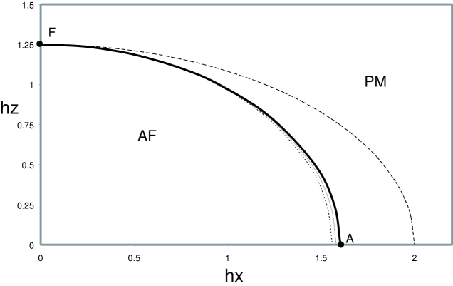
Figure 1: The ground state phase diagram of the model (1) for $\Delta=0.25$. The transition line between the antiferromagnetic (AF) and paramagnetic (PM) states obtained in the MFA is shown by thick solid line and that in the classical approximation (9) by dashed line. Thin solid line denotes the classical line (10) and dotted line corresponds to separatrix line (see Sec.III).

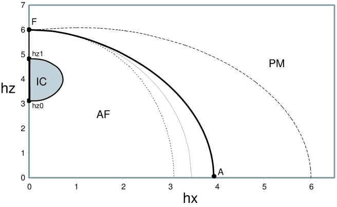
Figure 2: The ground state phase diagram of the model (1) for $\Delta=5$. The same notations as on Fig.1. The boundary of incommensurate critical (IC) phase is shown schematically (Sec.IV).

The case $\Delta>1$ can be analyzed in a similar way. In this case two-fold degenerated ground state in the AF phase is characterized by non-zero staggered magnetizations along the $X$ and $Z$ axes. But the expression for the transition line is rather cumbersome and we do not present it here. The transition line in the classical approximation for $\Delta=5$ is shown on Fig.2.

As it is known classical there is a remarkable, so-called ‘classical’ or disorder, line which lies in the AF region in the ($h_{x},h_{z}$) plane and is given by the equation:

$$\frac{h_{z}^{2}}{\left(1+\Delta\right)^{2}}+\frac{h_{x}^{2}}{2\left(1+\Delta\right)}=1$$ (10)

The classical line is remarkable in a sense that the ground state on it is identical to the classical one and quantum fluctuations are missing. It was shown in classical that the ground state of (1) on this line is two-fold degenerated and the exact ground state wave functions have the product form (3) and (4).

The ground state energy on the classical line for any even $N$ is

$$\frac{E}{N}=-\frac{1}{2}-\frac{\Delta}{4}$$ (11)

From Eqs.(7) one can find that in the case $\left|\Delta\right|<1$ the magnetizations on the classical line are:

$$\left\langle S_{n}^{z}\right\rangle = \frac{1}{2}\frac{h_{z}}{1+\Delta}$$

$$\left\langle S_{n}^{x}\right\rangle = \frac{h_{x}}{4}$$

$$\left\langle S_{n}^{y}\right\rangle = \left(-1\right)^{n}\frac{h_{x}}{4}\sqrt{\frac{1-\Delta}{1+\Delta}}$$ (12)

For $\Delta>1$ the parameters $A_{1}$and $A_{2}$ on the classical line are

$$A_{1,2}=\frac{1+\Delta+h_{z}}{h_{x}}\left(1\pm\sqrt{\frac{\Delta-1}{\Delta+1}}\right)$$ (13)

and the magnetizations on two sublattices are

$$\left\langle S_{n}^{x}\right\rangle_{1,2} = \frac{A_{1,2}}{A_{1,2}^{2}+1}$$

$$\left\langle S_{n}^{z}\right\rangle_{1,2} = \frac{1}{2}\frac{A_{1,2}^{2}-1}{A_{1,2}^{2}+1}$$

$$\left\langle S_{n}^{y}\right\rangle_{1,2} = 0$$ (14)

Thus, the classical approach shows that the ground state is different in the regions with $\left|\Delta\right|<1$ and $\Delta>1$. For $\left|\Delta\right|<1$ the classical ground state is given by a configuration, where the spins on odd and even sites pointing respectively at angles $\chi$ and $-\chi$ with respect to the $XZ$ plane. For $\Delta>1$ in the ground state all spin vectors lie in the $XZ$ plane with the spins on odd and even sites pointing respectively at angles $\varphi_{1}$ and $\varphi_{2}$ with respect to the $X$ axis. This means that besides uniform magnetizations along $X$ and $Z$ axes in the AF region there is as well the staggered magnetizations: in the $Y$ direction for $\left|\Delta\right|<1$ and in both $X$ and $Z$ directions for $\Delta>1$. ZZhxhz These facts are confirmed on the classical line, where the classical approximation gives exact ground state.

Of course, one can not expect that the classical approach gives accurate estimation of the transition line and correct description of the phase transition (critical exponents) XXZhx . Nevertheless, as it will be shown below the fact of the generation of the staggered magnetizations in the $Y$ direction for $\left|\Delta\right|<1$ and in both the $X$ and the $Z$ directions for $\Delta>1$ is qualitative true.

III Mean-field approximation

Previously, the mean-field approximation (MFA) has been proposed to study the anisotropic Heisenberg chain in the transverse magnetic field XXZhx ; Essler . It has been established that the MFA works very well if the transverse field is sufficiently strong and it gives qualitative results for intermediate fields. For $\Delta>-0.5$ the MFA allows to determine with high accuracy the critical transverse field at which the order-disorder transition occurs and to describe correctly the behavior of the system in the transition region. The MFA is based on the Jordan-Wigner transformation of spin-$1/2$ operators to the Fermi operators with the subsequent mean-field treatment of the Fermi Hamiltonian. In the case of coexisting transverse and longitudinal magnetic fields it is impossible to reduce the model Hamiltonian (1) to a local form in terms of the Fermi operators. Nevertheless, for this complicated case the MFA can be modified. In this section we develop the special version of the MFA, which remains the variational approach. This approach gives high accuracy in determining of the transition line and correctly describes the whole ground state phase diagram.

At first we perform a rotation of the spins in the $XZ$ plane by an angle $\varphi$:

$$S_{n}^{x} = \sigma_{n}^{x}\cos\varphi+\sigma_{n}^{z}\sin\varphi$$

$$S_{n}^{z} = -\sigma_{n}^{x}\sin\varphi+\sigma_{n}^{z}\cos\varphi$$

$$S_{n}^{y} = \sigma_{n}^{y}$$ (15)

where $\sigma_{n}^{\alpha}$ are new spin-$1/2$ operators.

The Hamiltonian (1) is transformed to the form

$$H = \sum\left(x\sigma_{n}^{x}\sigma_{n+1}^{x}+\sigma_{n}^{y}\sigma_{n+1}^{y}+z\sigma_{n}^{z}\sigma_{n+1}^{z}\right)-h\sum\sigma_{n}^{z}+H^{\prime}$$

$$H^{\prime} = \frac{1-\Delta}{2}\sin 2\varphi\sum\left(\sigma_{n}^{x}\sigma_{n+1}^{z}+\sigma_{n}^{z}\sigma_{n+1}^{x}\right)-\left(h_{x}\cos\varphi-h_{z}\sin\varphi\right)\sum\sigma_{n}^{x}$$ (16)

where

$$x = \cos^{2}\varphi+\Delta\sin^{2}\varphi$$

$$z = \Delta\cos^{2}\varphi+\sin^{2}\varphi$$

$$h = h_{z}\cos\varphi+h_{x}\sin\varphi$$ (17)

The angle $\varphi$ is a variational parameter over which we will minimize the ground state energy.

After Jordan-Wigner transformation to the Fermi operators $a_{n}^{+}$, $a_{n}$

$$\sigma_{n}^{+} = e^{i\pi\sum_{j<n}a_{j}^{+}a_{j}}a_{n}$$

$$\sigma_{n}^{z} = \frac{1}{2}-a_{n}^{+}a_{n}$$ (18)

the Hamiltonian (16) takes the form

$$H_{\mathrm{f}} = -\frac{hN}{2}+\frac{zN}{4}+\sum(h-z+\frac{1+x}{2}\cos k)a_{k}^{+}a_{k}$$ (19)

$$+ \frac{1-x}{4}\sum\sin k(a_{k}^{+}a_{-k}^{+}+a_{-k}a_{k})+z\sum a_{n}^{+}a_{n}a_{n+1}^{+}a_{n+1}+H_{\mathrm{f}}^{\prime}$$

We treat the Hamiltonian $H_{\mathrm{f}}$ in the MFA, which implies the decoupling of the four fermion term. The Fermi representation $H_{\mathrm{f}}^{\prime}$ has non-local form. But we note, that all terms in $H_{\mathrm{f}}^{\prime}$ contain odd number of the Fermi operators $a_{n}$ and, therefore, $\langle H_{\mathrm{f}}^{\prime}\rangle=0$ in the MFA. This fact holds the MFA in the frame of variational principle.

Thus, in the MFA the ground state energy $E_{0}$ and the one-particle excitation spectrum $\varepsilon(k)$ have the form:

$$E_{0}/N = -\frac{h}{2}+\frac{z}{4}+(h-z)\gamma_{1}+\frac{1+x}{2}\gamma_{2}+\frac{1-x}{4}\gamma_{3}+z\left(\gamma_{1}^{2}-\gamma_{2}^{2}+\gamma_{3}^{2}\right)$$ (20)

$$\varepsilon(k) = \sqrt{\left(u+v\cos k\right)^{2}+w^{2}\sin^{2}k}$$ (21)

where

$$u = h-z+2z\gamma_{1}$$

$$v = \frac{1+x}{2}-2z\gamma_{2}$$

$$w = \frac{1-x}{2}+2z\gamma_{3}$$ (22)

Quantities $\gamma_{1}$, $\gamma_{2}$ and $\gamma_{3}$ are the ground state expectation values, which are determined by the self-consistent equations:

$$\gamma_{1} = \langle a_{n}^{+}a_{n}\rangle=\int\limits_{0}^{\pi}\frac{\mathrm{d}k}{2\pi}\left(1-\frac{u+v\cos k}{\varepsilon(k)}\right)$$

$$\gamma_{2} = \langle a_{n}^{+}a_{n+1}\rangle=-\int\limits_{0}^{\pi}\frac{\mathrm{d}k}{2\pi}\frac{\left(u+v\cos k\right)\cos k}{\varepsilon(k)}$$

$$\gamma_{3} = \langle a_{n}^{+}a_{n+1}^{+}\rangle=-\int\limits_{0}^{\pi}\frac{\mathrm{d}k}{2\pi}\frac{w\sin^{2}k}{\varepsilon(k)}$$ (23)

The solution of the self-consistent equations (23) gives the minimum of the ground state energy (20) in a class of a ‘one-particle’ wave functions at a given angle $\varphi$. Thus, one should minimize the energy (20) with respect to the angle $\varphi$, solving the self-consistent equations (23) for each value of $\varphi$. This means that the proposed procedure remains variational one.

The physical meaning of the angle $\varphi$ is to show a direction of the total magnetization of the model (1)

$$S^{z} = \left\langle\sigma_{n}^{z}\right\rangle\cos\varphi=\left(\frac{1}{2}-\gamma_{1}\right)\cos\varphi$$

$$S^{x} = \left\langle\sigma_{n}^{z}\right\rangle\sin\varphi=\left(\frac{1}{2}-\gamma_{1}\right)\sin\varphi$$ (24)

Transforming the mean-field treated Fermi Hamiltonian back to the spin operators, we arrive to the well-studied anisotropic $XY$ model in a longitudinal magnetic field McCoy

$$H_{XY}=\sum\left[(v-w)\sigma_{n}^{x}\sigma_{n+1}^{x}+(v+w)\sigma_{n}^{y}\sigma_{n+1}^{y}\right]-u\sum\sigma_{n}^{z}$$ (25)

The model (25) has a transition line defined by the equation

$$u(h_{x},h_{z},\Delta)=v(h_{x},h_{z},\Delta)$$ (26)

which separates the region $u<v$ with the LRO represented by a staggered magnetization from the region $u>v$, where there is no LRO except the uniform magnetization (24). The transition line $h_{z\mathrm{c}}(h_{x},\Delta)$ is determined by the numerical solution of Eqs.(23),(26) with the minimization of the ground state energy over angle $\varphi$. The transition lines in the MFA for $\Delta=0.25$ and $\Delta=5$ are shown on Fig.1 and Fig.2 by thick solid lines.

It is well known McCoy that the critical properties of the model (25) belongs to the universality class of the two-dimensional Ising model. This means that in the MFA the gap is closed near the transition line linearly with the field and by the $1/8$ law for the staggered magnetization.

The MFA also shows, that for $\left|\Delta\right|<1$ ($w>0$) the model has a staggered magnetization along the $Y$ axis

$$\left\langle(-1)^{n}S_{n}^{y}\right\rangle=\frac{\left[w^{2}\left(v^{2}-u^{2}\right)\right]^{1/8}}{\sqrt{2\left(v+w\right)}}$$ (27)

while for $\Delta>1$ ($w<0$) the staggered magnetizations exist along the $X$ and the $Z$ axes

$$\ \left\langle(-1)^{n}S_{n}^{x}\right\rangle = \frac{\left[w^{2}\left(v^{2}-u^{2}\right)\right]^{1/8}}{\sqrt{2\left(v-w\right)}}\cos\varphi$$

$$\ \left\langle(-1)^{n}S_{n}^{z}\right\rangle = \frac{\left[w^{2}\left(v^{2}-u^{2}\right)\right]^{1/8}}{\sqrt{2\left(v-w\right)}}\sin\varphi$$ (28)

The validity of the 2D Ising type of the critical properties of the model (1) in the vicinity of the transition line has been checked by the density matrix renormalization group (DMRG) white calculations of the staggered magnetization and the gap. The staggered magnetization is computed as Essler

$$M_{st}^{\alpha}=\frac{1}{N}\left\langle 0\left|\sum(-1)^{n}S_{n}^{\alpha}\right|1\right\rangle\qquad\alpha=(x,y,z)$$ (29)

where $\left|0\right\rangle$ and $\left|1\right\rangle$ are two lowest energy states. These states are degenerate (at $N\longrightarrow\infty)$ in the ordered AF phase. Therefore, in the AF phase the gap is given by the second excited state, while in the disordered PM phase the ground state is non-degenerate and the first excitation determines the gap in the spectrum. We have performed the DMRG calculations using the infinite-size algorithm and open boundary conditions and the number of states $s$ kept in the DMRG truncating procedure is up to 25. We estimated the relative error due to DMRG truncation from difference between the data computed with $s=25$ and those with $s=20$ for chain lengths $N=202$. The estimated relative error is of the order of $10^{-5}$ which is sufficiently small for accurate estimates for the gap and the staggered magnetization. As an example, on Figs.3 and 4 we show the plots of $(M_{st}^{y})^{8}$ and the gap $m$ versus $h_{x}$ in the vicinity of the transition point for $\Delta=0.25$ and fixed $h_{z}=0.67$ (these parameters are related to those for the antiferromagnet $\mathrm{Cs}_{2}\mathrm{CoCl}_{4}$). A good linearity of the plotted data definitely confirms the 2D Ising character of the transition line. The excellent agreement between the DMRG and the MFA results on Fig.3 and Fig.4 shows high accuracy of the MFA. For example, the critical field $h_{x}$ estimated from the DMRG results differs from that obtained in the MFA within 0.04%.

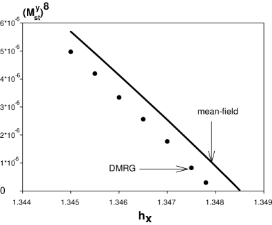
Figure 3: The staggered magnetization near the transition line as a function of $h_{x}$ for $\Delta=0.25$ and $h_{z}=0.67$.

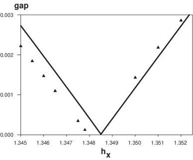
Figure 4: The gap as a function of $h_{x}$ near the transition line for $\Delta=0.25$ and $h_{z}=0.67$. (Solid line is the MFA, triangles are DMRG results extrapolated to the thermodynamic limit).

In addition to the transition line defined by Eq.(26), the Hamiltonian (25) contains another special line defined by the equation

$$u^{2}+w^{2}=v^{2}$$ (30)

This line separates the so-called ‘oscillatory’ region $u^{2}+w^{2}<v^{2}$ (lying totally in the AF phase), where spin correlators of the model (25) have oscillatory behavior with an incommensurate wavelength depending on the model parameters ($h_{x},h_{z},\Delta$), from the region without such oscillatory behavior of correlators McCoy . The line (30) is nothing but the classical line of the model (1). Remarkably, the MFA gives the exact ground state on the classical line. On this line the solution of Eqs.(23) has a simple form:

$$\sin^{2}\varphi=\frac{p}{1-p}\frac{1+\Delta}{1-\Delta}$$ (31)

where

$$p=\frac{h_{x}^{2}}{4}\frac{1-\Delta}{1+\Delta}$$ (32)

The values of $\gamma_{i}$ for $\left|\Delta\right|<1$ are

$$\gamma_{1}=\frac{1}{2}-\frac{\sqrt{1-p}}{2},\qquad\gamma_{2}=\gamma_{3}=-\frac{p}{4}$$ (33)

and for $\Delta>1$

$$\gamma_{1}=\frac{1}{2}-\frac{1}{2\sqrt{1-p}},\qquad\gamma_{2}=-\gamma_{3}=\frac{p}{4\left(1-p\right)}$$ (34)

The ground state energy is given by (11). Substituting Eqs.(31)-(34) into Eqs.(24),(27),(28) one can check that the magnetizations on the classical line in the MFA coincide with those given by Eqs.(12),(14).

The gap on the classical line in the MFA lies at $k=\pi$ and equals

$$m = 1-\frac{p}{2}-\sqrt{1-p},\qquad\left|\Delta\right|<1$$

$$m = \left(1-\frac{p}{2}-\sqrt{1-p}\right)\frac{1-2p-p\Delta}{\left(1-p\right)^{2}},\qquad\Delta>1$$ (35)

It is necessary to note that the elementary excitation in the AF phase can be regarded as a domain wall between the two AF ground states. In the cyclic chain these excitations are created in pairs in contrast to open chains. In Eq.(19) the end-chain correction term is omitted, and the spectrum Eq.(21) determines the gap for the open chain LSM ; Pfeuty . Therefore, in the AF region Eqs.(21),(35) give a half of the gap for a cyclic chain.

It is worth to mention one more special line on the phase diagram, so-called ‘separatrix’, defined by the equation

$$uv=v^{2}-w^{2}$$ (36)

This line separates the region $uv>v^{2}-w^{2}$, where the lowest excitation has momentum $k_{\min}=\pi$ from the region $uv<v^{2}-w^{2}$ (situated entirely in the AF phase), where the lowest excitation has momentum, depending on the model parameters as

$$\cos k_{\min}=\frac{uv}{w^{2}-v^{2}}$$

For any $\Delta$, the transition line $h_{z\mathrm{c}}(h_{x},\Delta)$, the classical line $h_{z\mathrm{cl}}(h_{x},\Delta)$ and the separatrix $h_{z\mathrm{s}}(h_{x},\Delta)$ lie in the following sequence (see Fig.1 and Fig.2)

$$h_{z\mathrm{s}}(h_{x},\Delta)\leq h_{z\mathrm{cl}}(h_{x},\Delta)\leq h_{z\mathrm{c}}(h_{x},\Delta)$$ (37)

All these lines meet each other in the only point F ($h_{x}=0,h_{z}=1+\Delta$).

III.1 The point F

The point F ($h_{x}=0$, $h_{z}=1+\Delta$) is the special boundary point, where all special lines terminate. The ground state in the point F is saturated ferromagnet. Near the point F ($h_{x}\ll 1$) the fermion density is small and the mean-field treatment of the four fermion term in Eq.(19) gives the accuracy, at least, up to $h_{x}^{4}$. We omit here intermediate calculations and give the final expressions for the special lines. The transition and the separatrix lines near the point F have the form:

$$h_{z\mathrm{c}}(h_{x},\Delta) = h_{z\mathrm{cl}}(h_{x},\Delta)+m_{\mathrm{cl}}+O\left(h_{x}^{6}\right)$$ (38)

$$h_{z\mathrm{s}}(h_{x},\Delta) = h_{z\mathrm{cl}}(h_{x},\Delta)-m_{\mathrm{cl}}+O\left(h_{x}^{6}\right)$$ (39)

where the behavior of the classical line $h_{z\mathrm{cl}}(h_{x},\Delta)$ is given by Eq.(10)

$$h_{z\mathrm{cl}}(h_{x},\Delta)=1+\Delta-\frac{h_{x}^{2}}{4}-\frac{h_{x}^{4}}{32\left(1+\Delta\right)}+O\left(h_{x}^{6}\right)$$ (40)

and $m_{\mathrm{cl}}$ is the gap near the point F on the classical line (see Eq.(35))

$$m_{\mathrm{cl}}=\frac{h_{x}^{4}}{128}\left(\frac{1-\Delta}{1+\Delta}\right)^{2}+O\left(h_{x}^{6}\right)$$ (41)

As one can see the difference between three special lines near the point F is very small, of the order of $h_{x}^{4}$.

The expressions for the gap are different to the left and to right of the separatrix line:

$$m = \frac{h_{x}^{2}}{4\sqrt{2}}\left|\frac{1-\Delta}{1+\Delta}\right|\sqrt{h_{z\mathrm{cl}}(h_{x},\Delta)-h_{z}},\qquad h_{z}<h_{z\mathrm{s}}$$

$$m = \left|h_{z}-h_{z\mathrm{c}}(h_{x},\Delta)\right|,\qquad h_{z}>h_{z\mathrm{s}}$$ (42)

The linear behavior of the gap in the vicinity of the transition line confirms the 2D Ising universality class of the transition line.

The staggered magnetizations in the vicinity of the point F vanish on two lines: on the transition line and on the line $h_{x}=0$. The Eqs.(24), (27), (28) near the point F reduce to

$$\left\langle S_{n}^{y}\right\rangle = (-1)^{n}B$$ (43)

$$B = \frac{1}{2}\left|\frac{1-\Delta}{1+\Delta}\right|^{1/4}\sqrt{h_{x}}\left(\frac{h_{z\mathrm{c}}-h_{z}}{2}\right)^{1/8}$$

for $\left|\Delta\right|<1$ and

$$\left\langle S_{n}^{x}\right\rangle = \frac{h_{x}}{4}+(-1)^{n}B$$

$$\left\langle S_{n}^{z}\right\rangle = \frac{1}{2}-\frac{(-1)^{n}}{2}h_{x}B$$ (44)

for $\Delta>1$.

To validate our analysis in the vicinity of the point F one should also estimate the effect of the part of the Hamiltonian $H^{\prime}$ in Eq.(16), omitted in the MFA. Near the point F the angle $\varphi\approx h_{x}/2$ and, therefore, these terms in $H^{\prime}$ are small and can be taking into account as perturbations. The corresponding perturbation theory contains only even orders. The estimate of the second order shows that the contribution of these terms to the ground state energy and to the gap is of the order of $h_{x}^{6}$ and $h_{x}^{2}(h_{z\mathrm{c}}-h_{z})$. This accuracy is sufficient to confirm the above equations.

We note that in the limit $\Delta\rightarrow\infty$ the point F transforms to the so-called multicritical point with macroscopic degeneracy of the ground state domb .

III.2 The point A

In the case $h_{z}=0$ the model (1) reduces to the anisotropic Heisenberg chain in the transverse magnetic field, which was studied in mori ; XXZhx ; Essler . At some value of magnetic field $h_{x\mathrm{A}}(\Delta)$ this model undergoes the transition from the antiferromagnetic state to the paramagnetic gapful state. We denote this transition point by the point A (see Figs.1 and 2).

To study the behavior of the system in the vicinity of the point A we shall follow the arguments of ZZhxhz , where the point A was analyzed in detail for the special case $\Delta\rightarrow\infty$. For $h_{x}=h_{x\mathrm{A}}(\Delta)$ and small longitudinal magnetic field $h_{z}$ we rewrite the Hamiltonian (1) in the form

$$H = H_{0}+V$$

$$H_{0} = \sum(S_{n}^{x}S_{n+1}^{x}+S_{n}^{y}S_{n+1}^{y}+\Delta S_{n}^{z}S_{n+1}^{z})-h_{x\mathrm{A}}(\Delta)\sum S_{n}^{x}$$

$$V = -h_{z}\sum S_{n}^{z}$$ (45)

The unperturbed Hamiltonian $H_{0}$ describes the transition point A, where the spectrum is gapless XXZhx .

As was mentioned above, the MFA does not give the transition point $h_{x\mathrm{A}}(\Delta)$ exactly (though with high accuracy), but it correctly describes the character of the transition. Therefore, we can use the MFA to determine how the small perturbation $V$ opens the gap. [We note, that the minimum of the MFA ground state energy at the point A is achieved at the angle $\varphi=\pi/2$ and two ‘bad’ terms in $H^{\prime}$ in Eq.(16) disappear at this point.]

To study the perturbation theory with small perturbation $V$ one can repeat step by step the analysis done for the special case $\Delta\rightarrow\infty$ of the model (45) ZZhxhz . As a result one finds that the perturbation theory contains infrared divergencies, which are absorbed in the scaling parameter $y=h_{z}^{2}N$. The perturbation series for the mass gap has the form

$$m=a(\Delta)h_{z}^{2}+g\left(\Delta,y\right)h_{z}^{2}$$ (46)

where $a(\Delta)$ is the second order correction and $g\left(\Delta,y\right)$ is the scaling function accumulated all high-order divergent terms. The scaling function $g\left(\Delta,y\right)$ in the thermodynamic limit ($y\rightarrow\infty$) tends to some finite limit. So, the gap takes the form

$$m=\left[a(\Delta)+g\left(\Delta,\infty\right)\right]h_{z}^{2}$$ (47)

From the last equation we see that the gap is proportional to $h_{z}^{2}$, but the factor at $h_{z}^{2}$ is given not only by the second order correction $a(\Delta)$ but by all collected divergent orders of the perturbation series.

For a fixed value of $\Delta$ the behavior of the transition line in ($h_{x},h_{z}$) plane near the point A can be found from the following consideration. As it was established above in the vicinity of the transition line the gap is proportional to the deviation from the line. This is valid for any direction of deviation except the direction at a tangent to the transition line. Thus, in the vicinity of the point A on the line $h_{x}=h_{x\mathrm{A}}(\Delta)$, the gap is

$$m\sim h_{x\mathrm{A}}(\Delta)-h_{x\mathrm{c}}(h_{z},\Delta)$$ (48)

On the other hand, the gap is given by Eq.(47). Equalizing these two expressions for the gap we obtain the equation for the transition line in the vicinity of the point A as

$$h_{x\mathrm{c}}(h_{z},\Delta)=h_{x\mathrm{A}}(\Delta)-f(\Delta)h_{z}^{2}$$ (49)

where the function $f(\Delta)$ is generally unknown and can be found numerically only.

Summarizing all above, we conclude that the MFA correctly describes the critical properties of the transition line and determines the transition line with high accuracy. This is because the MFA gives the exact ground state on the classical line, which is close to the transition line. Besides, the MFA is asymptotically exact in the vicinity of the point F. Therefore, for any value of $\Delta$, the accuracy in determining of the transition line drops as one moves from the point F to the point A. The MFA quality for the case $h_{z}=0$ was investigated in XXZhx ; Essler , where it was shown that the accuracy of the MFA is high for $\Delta>-0.5$, and the MFA fails in the limit $\Delta\rightarrow-1$ (where the accuracy decreases to 20%). Besides, the high accuracy of the MFA in the vicinity of the transition line is confirmed by DMRG calculations (see Fig.3 and Fig.4). The MFA qualitative correctly describes the line $h_{x}=0$ (no gap and sound-like spectrum for $h_{z}<1+\Delta$), but one can not expect that the MFA gives correct critical exponents in low-$h_{x}$ region.

IV The low-$h_{x}$ region

On the line $h_{x}=0$ the model (1) reduces to the well-known exactly solvable $XXZ$ model in the longitudinal magnetic field. In this model three phases exist in different ranges of the magnetic field $h_{z}$: the ferromagnetic (F) phase at $h_{z}>1+\Delta$; the antiferromagnetic (AF) phase at $0<h_{z}<h_{z0}(\Delta)$ ($h_{z0}(\Delta)$ is a lower critical field Gaudin ) and the critical phase at $0<h_{z}<1+\Delta$ ($|\Delta|<1$) and $h_{z0}(\Delta)<h_{z}<1+\Delta$ ($\Delta>1$) (see Fig.5).

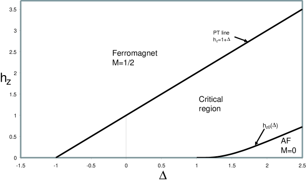
Figure 5: The ground state phase diagram of the $XXZ$ model in longitudinal magnetic field.

In the F phase the ground state is saturated ferromagnet $M\equiv\left\langle S_{n}^{z}\right\rangle=1/2$ with a gap in the spectrum. In this region the appearance of the transverse magnetic field does not cause noticeable change in the system properties. It results in appearance of a uniform magnetization in the $X$ direction and small decreasing of the magnetization in the $Z$ direction.

In the AF region the system is in a gapful phase with the long-range Neel order $M_{st}^{z}$ and zero uniform magnetization $M=0$. Due to the gap in the spectrum the effect of the $X$ component of magnetic field in the AF region can be obtained in the frame of a regular perturbation theory in $h_{x}$. The estimate of the first and the second orders in $h_{x}$ indicates the appearance of the uniform magnetizations in both the $X$ and the $Z$ directions and the staggered magnetization in the $X$ direction as

$$\left\langle S_{n}^{x}\right\rangle \sim h_{x}+(-1)^{n}h_{z}h_{x}$$

$$\left\langle S_{n}^{z}\right\rangle \sim (-1)^{n}M_{st}^{z}+h_{z}h_{x}^{2}$$ (50)

As follows from the last equations, in the case $h_{z}=0$ the applied transverse magnetic field does not cause the uniform magnetizations in the $Z$ direction and the staggered magnetization in the $X$ direction XXZhx .

The critical phase is characterized by non-zero magnetization $0<M<1/2$ in the ground state and by the massless spectrum. The low-energy properties in this phase are described by a free massless boson field theory with the Hamiltonian

$$H_{0}=\frac{v}{2}\int\mathrm{d}x\left[(\partial_{x}\Theta)^{2}+(\partial_{x}\Phi)^{2}\right]$$ (51)

where $\Phi(x)$ and $\Theta(x)$ are boson and dual field, respectively and $v(\Delta,h_{z})$ is the renormalized spin-wave velocity.

The spin-density operators are represented as book

$$S_{n}^{z} \simeq M+\frac{1}{2\pi R}\partial_{x}\Phi+a_{1}(-1)^{n}\cos\left(\frac{\Phi}{R}+2\pi Mx\right)$$

$$S_{n}^{x} \simeq b_{0}(-1)^{n}\cos\left(2\pi R\Theta\right)+b_{1}\cos\left(2\pi R\Theta\right)\cos\left(\frac{\Phi}{R}+2\pi Mx\right)$$ (52)

where $a_{1},b_{0}$ and $b_{1}$ are some constants Hikihara and we identify the site index $n$ with the continuous space variable $x$. The magnetization $M(\Delta,h_{z})$ and the compactification radius $R(\Delta,M)$ are functions of $\Delta$ and $h_{z}$ and can be determined by solving Bethe-ansatz integral equations BIK ; Cabra .

Both terms of operator $S^{x}$ in Eq.(52) are oscillating when $M\neq 0$ and are not relevant to the uniform $X$-component of the magnetic field. But as was shown in Nersesyan the second term in Eq.(52) corresponding to perturbation

$$V_{0}=h_{x}b_{1}\cos\left(2\pi R\Theta\right)\cos\left(\frac{\Phi}{R}+2\pi Mx\right)$$ (53)

has conformal spin $S=1$ and generates two other perturbations with zero conformal spin:

$$V_{1} = g_{1}\cos\left(4\pi R\Theta\right)$$

$$V_{2} = g_{2}\cos\left(\frac{2\Phi}{R}+4\pi Mx\right)$$ (54)

with $g_{1}\sim h_{x}^{2}$ and $g_{2}\sim h_{x}^{2}$.

The scaling dimensions of perturbations $V_{1}$, $V_{2}$ are $2\eta$ and $2/\eta$ ($\eta=2\pi R^{2}$), respectively. The perturbation $V_{2}$ describes Umklapp processes and it is responsible for the gap generation in the AF region, where $M=0$. But in the critical region ($h_{z}>0$) the magnetization $M\neq 0$ and the perturbation $V_{2}$ as well as the operator $V_{0}$ does not conserve the total momentum and will be frozen out.

Therefore, in the uniform longitudinal magnetic field $h_{z}$ the critical exponent for the mass gap is determined by the only non-oscillating perturbation $V_{1}$:

$$m\sim h_{x}^{\frac{1}{1-\eta}}$$ (55)

We note that in the special case $h_{z}=0$ ($|\Delta|<1$) the magnetization $M=0$ and all perturbations $V_{0}$, $V_{1}$ and $V_{2}$ are non-oscillated Bocquet . In this case in the region $\Delta>\cos[\pi\sqrt{2}]\approx-0.266$ the perturbation $V_{0}$ becomes most relevant and determines the mass gap as XXZhx

$$m\sim h_{x}^{\frac{2}{4-\eta-1/\eta}}$$ (56)

The perturbation $V_{1}$ corresponds to the spin-nonconserving operator $\sum(S^{x}_{n}S^{x}_{n+1}-S^{y}_{n}S^{y}_{n+1})$.book This means that the behavior of the system (1) at small $h_{x}$ is similar to that of well studied $XYZ$ chain in magnetic field $h_{z}$ with small anisotropy in $XY$ plane Giamarchi . Using the results of Ref.Giamarchi we conclude that in the region $\Delta>1$ the presence of small $X$-component of magnetic field leads to a sequence of three transitions with increasing longitudinal magnetic field $h_{z}$. The first one occurs at $h_{z0}(\Delta)$ ($\eta=2$), where the AF phase transforms to the incommensurate critical (IC) or ‘floating’ phase (see Fig.2). In the IC phase the perturbation $V_{1}$ is irrelevant and the spectrum remains gapless. Here the correlation functions display a power-law decay with a magnetization dependent wave vector. There is no LRO in the IC phase, except uniform magnetizations $M$ and $\left\langle S_{n}^{x}\right\rangle=\chi_{x}h_{x}$ (the susceptibility $\chi_{x}$ is finite in the critical phase). Unfortunately, neither the field theory approach nor the MFA allow us to determine the boundary of the IC phase. Therefore, this phase boundary is shown on Fig.2 schematically.

Further increasing of $h_{z}$ leads to the transition of the Kosterlitz-Thouless type taking place at the point $h_{z1}(\Delta)$ where $\eta=1$. At $h_{z}>h_{z1}(\Delta)$ the perturbation $V_{1}$ becomes relevant ($\eta<1$) and the system crosses from the IC phase to a strong-coupling regime with the staggered magnetizations in both $X$ and $Z$ directions (AF phase).

The last transition with further increasing of $h_{z}$ occurs near the point F at $h_{z}=h_{zc}$ (see Fig.2). This transition to the PM phase was studied in Sec.III.

The field theory approach allows also to determine the exponent for the appeared LRO. The transverse magnetic field generates the staggered magnetization along the $Y$ axis at $\left|\Delta\right|<1$ as

$$\left\langle S_{n}^{y}\right\rangle\sim\frac{(-1)^{n}}{\xi^{\eta/2}}\sim(-1)^{n}m^{\eta/2}\sim(-1)^{n}h_{x}^{\eta/(2-2\eta)}$$ (57)

and along $X$ and $Z$ axes at $\Delta>1$ and $h_{z1}(\Delta)<h_{z}<1+\Delta$

$$\left\langle S_{n}^{x}\right\rangle \sim \chi_{x}h_{x}+(-1)^{n}h_{x}^{\eta/(2-2\eta)}$$

$$\left\langle S_{n}^{z}\right\rangle \sim M+(-1)^{n}h_{x}^{(2-\eta)/(2-2\eta)}$$ (58)

We note, that in the limit $h_{z}\to 1+\Delta$ ($\eta\to 1/2$), the exponents for the mass gap (55) and staggered magnetizations in Eqs.(57),(58) agree with the MFA results in Eqs.(42),(43),(44).

The staggered magnetization along the $Z$ axis in Eq.(58) can be derived in the same manner as was derived the generated perturbations $V_{1}$ and $V_{2}$ in Eqs.(54). According to Eqs.(52) the non-zero contribution to the first order correction in $h_{x}$ to the staggered magnetization $\left\langle(-1)^{n}S_{n}^{z}\right\rangle$ is given by the following terms in spin-density operators

$$(-1)^{n}S_{n}^{z} \sim \cos\left(\frac{\Phi}{R}+2\pi Mx\right)$$

$$S_{n}^{x} \sim \cos\left(2\pi R\Theta\right)\cos\left(\frac{\Phi}{R}+2\pi Mx\right)$$ (59)

Then the leading contribution comes from small distances of order of ultraviolet cut-off (the lattice constant)

$$(-1)^{x_{1}}S^{z}(z_{1}) \sim h_{x}\int d^{2}z_{2}e^{\mathrm{i}2\pi M(x_{2}-x_{1})}\exp[-\mathrm{i}\frac{\Phi(z_{1})}{R}]\exp[\mathrm{i}\frac{\Phi(z_{2})}{R}]\cos[2\pi R\Theta(z_{2})]$$ (60)

$$\sim h_{x}\cos[2\pi R\Theta(z_{1})]\sim h_{x}(-1)^{x_{1}}S^{x}(z_{1})$$

Thus, the relation between the staggered magnetization along $X$ and $Z$ axes is established

$$\left\langle(-1)^{n}S_{n}^{z}\right\rangle\sim h_{x}\left\langle(-1)^{n}S_{n}^{x}\right\rangle$$ (61)

which results in the critical exponent for $\left\langle(-1)^{n}S_{n}^{z}\right\rangle$ written in Eq.(58).

IV.1 Perturbation theory. Mapping to the $XYZ$ model in the magnetic field

In this subsection we study the behavior of the model in the critical phase from the perturbation theory point of view. In some sense this subsection is complementary to the field theory approach.

For a small $X$ component of a magnetic field the Hamiltonian (1) can be written in the form

$$H = H_{0}+V$$

$$H_{0} = \sum(S_{n}^{x}S_{n+1}^{x}+S_{n}^{y}S_{n+1}^{y}+\Delta S_{n}^{z}S_{n+1}^{z})-h_{z}\sum S_{n}^{z}$$

$$V = -h_{x}\sum S_{n}^{x}$$ (62)

As was said above in the critical region (5) the model $H_{0}$ is in the critical regime with non-zero magnetization $M$.

The transition operator $S^{x}=\sum S_{n}^{x}$ in $V$ conserves the momentum and changes the total $S^{z}$ by one. Therefore, since the unperturbed Hamiltonian $H_{0}$ conserves the value of $S^{z}$, the perturbation theory in $V$ contains only even orders.

The operator $V$ acting on the ground state or the low-lying states produces states with ‘high’ energies $E_{s}-E_{0}\equiv\varepsilon_{s}\gtrsim 1$. So, the perturbation theory in $V$ has such a ‘two-level’ structure with alternate low-lying and high-lying intermediate states. As a result the denominator of the $2n$-th perturbation order contains $n$ factors with ‘high’ excitation energies $\varepsilon_{s}\gtrsim 1$ and ($n-1$) with low-lying excitation $\varepsilon_{s}\sim 1/N$.

Omitting numerical factors, in all orders of perturbation theory one can take out all ‘high’ energies from the denominator and sum up over all high-lying intermediate states. As a result, we arrive at the perturbation theory with the effective perturbation

$$V^{\prime}=-h_{x}^{2}\sum S_{n}^{x}S_{m}^{x}$$ (63)

We note, that the perturbation theory with the perturbation $V^{\prime}$ coincides with the original perturbation theory (62) in a sense, that both perturbation series have the same order of divergencies (or power of $N$) at each order in $h_{x}$. But numerical factors at each order in $h_{x}$ can be different.

The behavior of the ground state correlation function $\left\langle S_{n}^{x}S_{n+r}^{x}\right\rangle$ of the model $H_{0}$ on large distances is known Hikihara

$$\left\langle S_{n}^{x}S_{n+r}^{x}\right\rangle=A_{0}(\eta)\frac{(-1)^{r}}{r^{\eta}}-A_{1}(\eta)\frac{\cos\left(2\pi Mr\right)}{r^{\eta+1/\eta}}$$ (64)

and, therefore, due to oscillation of the correlator $\left\langle S_{n}^{x}S_{m}^{x}\right\rangle$ (for $M\neq 0$) the sum over $n$ and $m$ can be approximately estimated as a one half of the first term:

$$\sum_{n,m}\left\langle S_{n}^{x}S_{m}^{x}\right\rangle=\frac{N}{4}+2\sum_{n>m}\left\langle S_{n}^{x}S_{m}^{x}\right\rangle\simeq\frac{N}{4}+\sum_{n}\left\langle S_{n}^{x}S_{n+1}^{x}\right\rangle$$ (65)

The last equation suggests that the perturbation $V^{\prime}$ can be reduced to the operator $V^{\prime\prime}$

$$V^{\prime\prime}=-ah_{z}^{2}N-bh_{z}^{2}\sum S_{n}^{x}S_{n+1}^{x}$$ (66)

with some constants $a,b$. In order to verify this assumption we compared the matrix elements of the operator $V^{\prime\prime}$ with those of $V^{\prime}$. We have found that the dependence of the matrix elements of the operators $V^{\prime}$ and $V^{\prime\prime}$ on $N$ is identical.

As a result of the analysis we arrive at the effective Hamiltonian

$$H_{\mathrm{eff}}=-aNh_{x}^{2}+\sum\left((1-bh_{x}^{2})S_{n}^{x}S_{n+1}^{x}+S_{n}^{y}S_{n+1}^{y}+\Delta S_{n}^{z}S_{n+1}^{z}\right)-h_{z}\sum S_{n}^{z}$$ (67)

Again, the original model (62) is equivalent to the effective model (67) in a sense, that the perturbation series for both models have the same order of divergencies at each order of $h_{z}$. This fact means that the effective model has the same critical exponents as the original model (62).

One can see, that the effective perturbation $V^{\prime\prime}$ is nothing but the generated perturbation $V_{1}$ found in bosonization technique Eq.(54) with $g_{1}=bh_{x}^{2}$. So, the above analysis represents another way to obtain an effective perturbation responsible for the most divergent part in the perturbation theory.

Unfortunately, the effective model (67) is not exactly solvable one in general case. But it can be used for checking the bosonization expression for the mass gap (55) in two special cases $h_{z}=0$ and $\Delta=0$, where the effective model reduces to integrable $XYZ$ model and $XY$ model in magnetic field, respectively. In these special cases the exact expressions for the mass gap are known McCoy ; Baxter . They confirm the validity of the critical exponent in Eq.(55).

V Special case $\Delta=-1$

When $\Delta\rightarrow-1$ the point F tends to zero, and exactly on the line $\Delta=-1$ both classical and transition lines disappear. In the vicinity of the line $\Delta=-1$ it is convenient to rotate the coordinate system in such a way that the Hamiltonian (1) takes the form

$$H = H_{0}+V_{h}+V_{\Delta}$$

$$H_{0} = -\sum\mathbf{S}_{n}\cdot\mathbf{S}_{n+1}-h_{x}\sum(-1)^{n}S_{n}^{z}$$

$$V_{h} = -h_{z}\sum S_{n}^{x}$$

$$V_{\Delta} = (1+\Delta)\sum S_{n}^{x}S_{n+1}^{x}$$ (68)

The unperturbed Hamiltonian $H_{0}$ describes the critical behavior of the system at $0<h_{x}<h_{0}$, Alkaraz where the estimate of $h_{0}$ is $h_{0}\approx 0.53(3)$. XXZhx The spin-density operators of $H_{0}$ are related to the bosonic fields by Eqs.(52) with $M=0$, where the compactification radius $R(h_{x})$ is a function of $h_{x}$. This dependence is generally unknown, but the limiting values of $\eta(h_{x})=2\pi R^{2}(h_{x})$ are known XXZhx

$$\eta\left(h_{x}\right) = \frac{h_{x}}{\pi},\qquad h_{x}\rightarrow 0$$

$$\eta\left(h_{x}\right) = \frac{1}{4},\qquad h_{x}\rightarrow h_{0}$$ (69)

The perturbations $V_{h}$ and $V_{\Delta}$ have scaling dimensions $\eta/2$ and $2\eta$, respectively. Therefore, according to Eqs.(69) both perturbations $V_{h}$ and $V_{\Delta}$ are relevant in the critical region $0<h_{x}<h_{0}$ and produce a mass gaps

$$m_{h} \sim h_{z}^{1/(2-\eta/2)}$$

$$m_{\Delta} \sim \left|1+\Delta\right|^{1/(2-2\eta)}$$ (70)

In particular, $m_{h}\sim\sqrt{h_{z}}$, $m_{\Delta}\sim\sqrt{\left|1+\Delta\right|}$ at $h_{x}\to 0$ and $m_{h}\sim h_{z}^{8/15}$, $m_{\Delta}\sim\left|1+\Delta\right|^{2/3}$ at $h_{x}\to h_{0}$.

The gap at $\Delta=-1$ and for $h_{x},h_{z}<<1$ can be asymptotically exactly described by the spin-wave theory XXZhx . The validity of the spin-wave approximation is quite natural because the number of magnons forming the ground state is small for $h_{x},h_{z}<<1$. The spin-wave result for the gap is

$$m=\sqrt{h_{z}(h_{z}+\frac{h_{x}^{2}}{2})}$$ (71)

For $h_{z}<<h_{x}^{2}<<1$ Eq.(71) agrees with the conformal theory result Eq.(70) at $\eta\to 0$ and gives the preexponential factor for the gap.

VI Discussion and conclusion

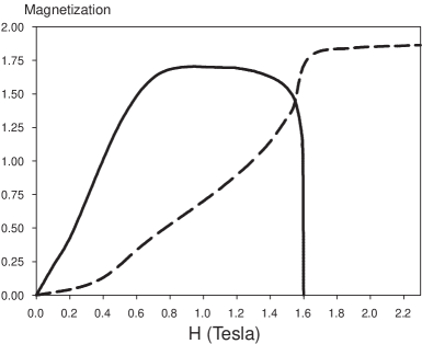
Figure 6: Uniform (dashed line) and staggered (solid line) magnetization curves.

As it was mentioned the order-disorder transition induced by the magnetic field has been observed in the quasi-one-dimensional antiferromagnet $\mathrm{Cs}_{2}\mathrm{CoCl}_{4}$ described, as supposed, by the model (1) with $\Delta=0.25.$ It is interesting to compare the magnetization curves obtained in neutron-scattering experiment kenz with those in the MFA. In this experiment the magnetic field $H$ has been applied at an angle $\beta\simeq 40^{0}$ to the $XY$ plane. This means that $H_{x}\simeq H_{z}\simeq H/\sqrt{2}.$ According to kenz $g$-factors in $\mathrm{Cs}_{2}\mathrm{CoCl}_{4}$ are $g_{x,y}=2g_{z}=4.80$. Therefore, the ratio of the effective fields in the model (1) is $\frac{h_{x}}{h_{z}}=\frac{2H_{x}}{H_{z}}\simeq 2$. The total magnetization $M_{tot}$ is

$$M_{tot}=\frac{\mu_{b}}{\sqrt{2}}\left(g_{x}\langle S_{n}^{x}\rangle+g_{z}\langle S_{n}^{z}\rangle\right)$$ (72)

where $\langle S_{n}^{x}\rangle$ and $\langle S_{n}^{z}\rangle$ are the magnetizations calculated in the MFA at the effective fields $h_{x}=2h_{z}$. The AF ordered moment is given by $M_{st}=g_{y}\mu_{b}\langle\left|(-1)^{n}S_{n}^{y}\right|\rangle$. On Fig.6 we plot $M_{tot}$ and $M_{st}$ as the functions of the magnetic field $H$ ($H=\frac{\sqrt{2}h_{x}J}{g_{x}\mu_{b}})$. These magnetization curves are qualitative similar to the experimental ones (Figs.12 and 14 in Ref.kenz ). The maximal value of staggered magnetization $1.7\mu_{b}$ agrees with the experimental magnitude of the AF ordered moment 1.6$\mu_{b}$. The total magnetization at $H\rightarrow\infty$ in the MFA $M_{tot}=1.9\mu_{b}$ is consistent with the saturation moment $1.7\mu_{b}$ estimated in kenz . At the same time, there is essential difference in the low-field behavior of $M_{st}$. The experimental AF ordered moment is finite at $H=0$, while $M_{st}=0$ at $H=0$ on Fig.6. This difference is due to weak interchain couplings, which form the magnetically ordered ground state in the real compound at $H=0$ and this effect is absent in the one-dimensional model (1). The behavior of the magnetizations in the vicinity of the critical field on Fig.6 is similar to the experimental curve. But the value of the critical field on Fig.6 is $1.6T$, while the experimental value is $2.1T$. We do not believe that the MFA is the reason for this discrepancy. The possible reason may lie in the fact that $\mathrm{Cs}_{2}\mathrm{CoCl}_{4}$ is described by the $s=\frac{3}{2}$ antiferromagnetic model with strong single-ion anisotropy and its reducing to the $s=\frac{1}{2}$ model is approximate.

Magnetic measurements in kenz were performed in the field applied at a fixed angle $\beta$ to the anisotropy axis. It is interesting to consider how the properties of the model (1) is changed when the magnetic field is turned from purely longitudinal ($\beta=0$) to transverse direction ($\beta=\frac{\pi}{2}$). If the effective field $h$ is in the range $(1+\Delta)<h<h_{x\mathrm{A}}(\Delta)$ for $\left|\Delta\right|<1$ or $h_{x\mathrm{A}}(\Delta)<h<(1+\Delta)$ for $\Delta>1$ then there is the critical angle $\beta_{0}$, which is defined by the intersection of the circle $h_{x}^{2}+h_{z}^{2}=h^{2}$ with the transition line. At this angle the phase transition from the $AF$ phase at $\beta>\beta_{0}$ ($\beta<\beta_{0})$ for $\Delta<1$ ($\Delta>1)$ to $PM$ phase at $\beta<\beta_{0}$ ($\beta>\beta_{0})$ takes place. The staggered magnetization and the gap vanish at $\beta=\beta_{0}$ as $M_{st}\sim\left|\beta-\beta_{0}\right|^{1/8}$ and $m\sim\left|\beta-\beta_{0}\right|$.

In conclusion, we have studied the spin-$\frac{1}{2}$ $XXZ$ Heisenberg chain in the mixed longitudinal and transverse magnetic field. It was shown that the ground state phase diagram on the $(h_{x},h_{z})$ plane contains the $AF$ and the $PM$ phases separated by the transition line. The transition line was determined using the proposed special version of the MFA, which reduces the $XXZ$ model in the mixed fields to the $XY$ model in the uniform longitudinal field. The MFA gives the transition line with high accuracy at least for $\Delta\geq-0.5$. This fact is confirmed by comparison of the MFA results with DMRG calculations. The MFA gives satisfactory description of the whole phase diagram, though the critical exponents of low-$h_{x}$ dependence of the gap and the magnetization can not be found correctly in the MFA. These exponents have been found with use of the conformal field method.

The field theory approach also shows that in the region $\Delta>1$ the phase diagram contains IC or floating phase characterized by the gapless spectrum and power-low decay of correlation functions. The form of the boundary of IC phase can be determined numerically only. But this boundary is located certainly on the left of the classical line, where the spectrum is gapped.

We believe that the modified MFA is suitable for the studying of the magnetic phase transitions of the quasi-one dimensional anisotropic magnets induced by the applied magnetic field. The important problem is to take into account effects of inter-chain interactions Q1D .

We thank Dr.V.Cheranovskii for useful discussions. This work was supported under RFBR Grant No 03-03-32141 and ISTC No 2207.

References

- (1) D.C.Dender, P.R.Hammar, D.H.Reich, C.Broholm and G.Aeppli, Phys.Rev.Lett. 79, 1750 (1997).
- (2) R.Helfrich, M.Koppen, M.Lang, F.Steglich and A.Ochiku, J.Magn.Magn.Mat. 177, 309 (1998).
- (3) M.Kohgi, K.Iwasa, J.-M.Mignot, B.Fåk, P.Gegenwart, M.Lang, A.Ochiai, H.Aoki, and T.Suzuki, Phys. Rev. Lett. 86, 2439 (2001).
- (4) I.Affleck and M.Oshikawa, Phys.Rev.B 60, 1038 (1999).
- (5) J.Lou, S.Qin, C.Chen, Z.Su and L.Yu, Phys.Rev.B 65, 064420 (2002).
- (6) F.H.L.Essler, A.Furusaki and T.Hikihara, Phys.Rev.B 68, 064410 (2003).
- (7) M.Kenzelmann, R.Coldea, D.A.Tennant, D.Visser, M.Hofmann, P.Smeibidl, and Z.Tylczynski, Phys. Rev. B 65, 144432 (2002).
- (8) G.Uimin, Y.Kudasov, P.Fulde and A.A.Ovchinnikov, Eur.Phys.J.B 16, 241 (2000).
- (9) A.Dutta, D.Sen, Phys. Rev. B 67, 094435 (2002).
- (10) C.N.Yang and C.P.Yang, Phys.Rev.B 150, 321, 327 (1966).
- (11) S.Mori, J.-J.Kim and I.Harada, J.Phys.Soc.Jpn 64, 3409 (1995).
- (12) Y.Hieida, K.Okunishi and Y.Akutsu, Phys.Rev.B 64, 224422 (2001).
- (13) D.V.Dmitriev, V.Ya.Krivnov, A.A.Ovchinnikov and A.Langari, JETP 95, 538 (2002); D.V.Dmitriev, V.Ya.Krivnov and A.A.Ovchinnikov, Phys. Rev. B 65, 172409 (2002).
- (14) J.-S.Caux, F.H.L.Essler, U.Low, Phys.Rev.B 68, 134431 (2003).
- (15) P.Sen, Phys. Rev. E 63, 16112 (2001).
- (16) A.A.Ovchinnikov, D.V.Dmitriev, V.Ya.Krivnov, V.O.Cheranovskii, Phys. Rev. B 68, 214406 (2003).
- (17) J.Kurmann, H.Tomas and G.Muller, Physica A 112, 235 (1982); G.Muller and R.E.Shrock, Phys.Rev.B 32, 5845 (1985).
- (18) E.Barouch and B.M.McCoy, Phys. Rev. A 3, 786 (1971).
- (19) S.R.White, Phys. Rev. B 48, 10345 (1993).
- (20) E.Lieb, T.Schultz, D.Mattis, Ann. Phys. (N.Y.) 16, 407 (1961).
- (21) P.Pfeuty, Ann. Phys. (N.Y.) 57, 79 (1970).
- (22) C.Domb, Adv.Phys. 9, 149 (1960).
- (23) J.des Cloizeaux and M.Gaudin, J. Math. Phys. 7, 1384 (1966).
- (24) A.O.Gogolin, A.A.Nersesyan, A.M.Tsvelik, Bosonization and Strongly Correlated Systems (Cambridge University Press, Cambridge, 1998).
- (25) T.Hikihara and A.Furusaki, Phys.Rev. B69, 064427 (2004).
- (26) N.M.Bogoliubov, A.G.Izergin and V.E.Korepin, Nucl.Phys.B 275, 687 (1986).
- (27) D.C.Cabra, A.Honecker, P.Pujol, Phys.Rev.B 58, 6241 (1998).
- (28) A.A.Nersesyan, A.Luther and F.V.Kusmartsev, Phys.Lett.A 176, 363 (1993).
- (29) M.Bocquet, F.H.L.Essler, A.M.Tsvelik and A.O.Gogolin, Phys.Rev.B 64, 094425 (2001).
- (30) T.Giamarchi and H.J.Schulz, J. de Physique (Paris) 49, 819 (1988).
- (31) R.J.Baxter, Phys. Rev. Lett. 26, 834 (1971); R.J.Baxter, Ann. Phys. 70, 323 (1972).
- (32) F.C.Alcaraz and A.L.Malvezzi, J.Phys.A 28, 1521 (1995); M.Tsukano, K.Nomura, J.Phys.Soc.Jpn.67, 302 (1998).
- (33) D.V.Dmitriev and V.Ya.Krivnov, cond-mat/0407203.