Scaling of local interface width of statistical growth models

Abstract

We discuss the methods to calculate the roughness exponent $\alpha$ and the dynamic exponent $z$ from the scaling properties of the local roughness, which is frequently used in the analysis of experimental data. Through numerical simulations, we studied the Family, the restricted solid-on-solid (RSOS), the Das Sarma-Tamborenea (DT) and the Wolf-Villain (WV) models in one- and two dimensional substrates, in order to compare different methods to obtain those exponents. The scaling at small length scales do not give reliable estimates of $\alpha$, suggesting that the usual methods to estimate that exponent from experimental data may provide misleading conclusions concerning the universality classes of the growth processes. On the other hand, we propose a more efficient method to calculate the dynamic exponent $z$, based on the scaling of characteristic correlation lengths, which gives estimates in good agreement with the expected universality classes and indicates expected crossover behavior. Our results also provide evidence of Edwards-Wilkinson asymptotic behavior for the DT and the WV models in two-dimensional substrates.

1 Introduction

The comparison of morphological features of thin films’ surfaces and of those of discrete or continuum growth models is of fundamental importance to infer the basic mechanisms of the experimental growth processes [1, 2, 3]. Statistical models usually represent real systems’ features by simple stochastic processes, neglecting the details of the microscopic interactions, but still being able to reproduce their large scale properties. Frequently, the interest is to classify model systems and real surfaces into universality classes of interface growth. At this point it is essential that the theoretical systems be investigated in the same lines of the experimental work, i. e. by analyzing the same physical quantities with standard methods.

In the study of interface growth models, one usually is interested in the scaling properties of the global interface width. For a discrete deposition model in a $d$-dimensional substrate of length $L$, the global width is defined as

$$\xi(L,t)={\left[{\left<{{{1\over{L^{d}}}\sum_{i}{{\left(h_{i}-\overline{h}\right)}^{2}}}}\right>}\right]}^{1/2},$$ (1)

where $h_{i}$ is the height of column $i$ at time $t$, the bar in $\overline{h}$ denotes a spatial average and the angular brackets denote a configurational average. For short times (growth regime), $\xi$ is expected to scale as

$$\xi\sim t^{\beta},$$ (2)

and for long times (steady state) it saturates as

$$\xi_{sat}\left(L\right)\equiv\xi\left(L,t\to\infty\right)\sim L^{\alpha}.$$ (3)

The dynamical exponent is $z=\alpha/\beta$.

In numerical studies, the exponent $\beta$ is measured in the growth regime of very large substrates. The exponents $\alpha$ and $z$ are obtained from data in the steady states or approaching this long-time regime, in which the heights of the deposits ($\overline{h}\sim t\sim L^{z}$ or larger, with $z\geq 1$) significantly exceed their lateral lengths ($L$).

On the other hand, in experiments and in some theoretical works (analytical and numerical) one is interested in the scaling properties of local surface fluctuations during the growth regime, when $\overline{h}\ll L$ and, consequently, the effects of finite lateral sizes of the substrate are negligible. In these conditions, height fluctuations inside small windows (boxes) over a very large surface are measured. This is achieved by calculating the height-height correlation function $G\left(r,t\right)\equiv\left<{\overline{{\left(h_{i+r}-h_{i}\right)}^{2}}}\right>$ or the local interface width

$$w(r,t)\equiv{\langle{{\left<{\left[h_{i}-{\left<h\right>}_{r}\right]}^{2}\right>}_{r}}\rangle}^{1/2},$$ (4)

where ${\left<\dots\right>}_{r}$ denotes a spatial average over windows of size $r$. Usually, these windows are square boxes of side $r$ scanning the surface of the deposit. $\sqrt{G\left(r,t\right)}$ and $w(r,t)$ have the same scaling properties. In systems with normal scaling (in opposition to anomalous scaling), the local width scales as

$$w(r,t)\sim t^{\beta}f\left(r/t^{1/z}\right),$$ (5)

where $f$ is a scaling function. It is expected that

$$f(x)\to x^{\alpha},x\ll 1$$ (6)

and

$$f(x)\to const,x\gg 1.$$ (7)

In systems with anomalous scaling, Eq. (5) is still valid, but $f$ scales with $\alpha_{local}<\alpha$ for small $x$ (small $r$) [4] (it has been shown [5] that $\alpha_{local}\leq 1$).

Experimentally, the roughness exponent $\alpha$ is usually obtained from the scaling of the local width or the height-height correlation function at small length scales (Eq. 6). Some techniques have been developed to characterize a surface by using a few images of varying scan sizes or even only one image subdivided into windows of a given size. The scaling of the local roughness (Eqs. 5 and 6) is then used to estimate the exponent $\alpha$ [6, 7]. However, one of the main problems for the calculation of $\alpha$ is the narrow range in which $\log{w}$ increases approximately linearly with $\log{r}$. Sometimes that range does not exceed one order of magnitude. In some theoretical works, similar procedure was also adopted, although it is more common the calculation of $G\left(r,t\right)$ or $w\left(r,t\right)$ in the steady states, i. e. for very long deposition times [8]. Even then, the problem of a restricted scaling region (Eq. 6) is still present; see e. g. Ref. [9].

The first aim of this work is to study the scaling properties of the local interface width of several limited-mobility growth models in order to propose methods to calculate the scaling exponents from data in the growth regimes, i. e. for very large system sizes and relatively small times. The advantages or disadvantages of each method may guide the lines of investigation of the universality classes of real growth processes. One of our conclusions is that the accuracy of the estimate of the exponent $\alpha$ is very poor when it is calculated with a method that parallels the one used in experimental works, i. e. based on the scaling relation (6) for small length scales. For some theoretical models with weak corrections to scaling, this problem may be partially overcome with another method, but this method is not suitable for analyzing experimental data due to their typical error bars. On the other hand, we present a method to calculate the exponent $z$ from the local roughness scaling and discuss its advantages with application to some discrete models. We will show that, in experimental works where the interest is to search for the universality classes of the growth processes from local width data, the best choice seems to be the calculation of the exponent $z$ with that technique.

The models we will consider here are the random deposition with surface relaxation of Family [10], the restricted solid-on-solid (RSOS) model of Kim and Kosterlitz [11] and the molecular beam epitaxy models of Das Sarma and Tamborenea (DT model) [12] and of Wolf and Villain (WV model) [13], in $1+1$ and $2+1$ dimensions. From the theoretical point of view, the advantage of the method proposed here is that the computational cost is very much reduced when compared to a study in which one has to wait until the stationary regime is attained. Also, our results are particularly relevant to elucidate recent questions [14, 15] on the universality classes of the WV and the DT models in $2+1$ dimensions.

The rest of this work is organized as follows. In Sec. 2, we will briefly review the growth rules of the discrete models studied here, the continuum equations representing the expected universality classes and the simulation procedure. In Sec. 3, we will discuss the methods to estimate the roughness exponent in the growth regime. In Sec. 4, we will present the method to calculate the dynamical exponent. In Sec. 5 we will present our results for the DT and the WV models. In Sec. 6 we summarize our results and present our conclusions.

2 Models, universality classes and simulation procedure

We will simulate four limited mobility growth models whose stochastic aggregation rules are illustrated in Figs. 1a-d.

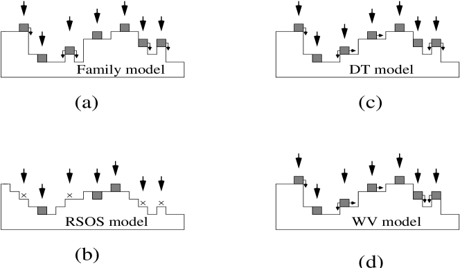
Figure 1: (a) The aggregation rules of the Family model, in which the relaxation of incident particles to their sticking positions is indicated by arrows. The incident particle in the middle has equal probabilities to stick at any one of the neighboring columns.(b) The aggregation rules of the $RSOS$ model, where the crosses indicate the rejected deposition attempts. c) The aggregation rules for the DT model, where the deposited particle seeks only to have one nearest neighbor and (d) for the WV model, where the particle will choose the site with the largest number of neighbors.

In the Family model [10] (Fig. 1a), a column of the deposit is randomly chosen and, if no neighboring column has a smaller height than the column of incidence, the particle sticks at the top of this one. Otherwise, it sticks at the top of the column with the smallest height among the neighbors. If two or more neighbors have the same minimum height, the sticking position is randomly chosen among them.

In the continuum limit, the Family model is expected to belong to the Edwards-Wilkinson (EW) universality class [17], i. e. its scaling properties are the same obtained from the linear EW equation

$${{\partial h}\over{\partial t}}=\nu{\nabla}^{2}h+\eta(\vec{x},t).$$ (8)

Here, $h$ is the height at the position $\vec{x}$ at time $t$, $\nu$ represents a surface tension and $\eta$ is a Gaussian noise [2, 18] with zero mean and variance $\langle\eta\left(\vec{x},t\right)\eta(\vec{x^{\prime}},t^{\prime})\rangle=D\delta^{d}(\vec{x}-\vec{x^{\prime}})\delta\left(t-t^{\prime}\right)$. The EW equation can be exactly solved ([17] - see also Ref. [3]), giving $\alpha=1/2$ in $d=1$ and $\alpha=0$ ($\xi^{2}\sim\ln{L}$) in $d=2$, while $z=2$ in all dimensions.

In the $RSOS$ model [11] (Fig. 1b), the incident particle may stick at the top of the column of incidence if the differences of heights between the incidence column and each of the neighboring columns do not exceed ${\Delta h}_{MAX}=1$. Otherwise, the aggregation attempt is rejected. Due to the dependence of the local growth rate on the local height gradient, the RSOS model is asymptotically represented by the Kardar-Parisi-Zhang equation [18]

$${{\partial h}\over{\partial t}}=\nu{\nabla}^{2}h+{\lambda\over 2}{\left(\nabla h\right)}^{2}+\eta(\vec{x},t),$$ (9)

where $\lambda$ represents the excess velocity. The exponents of the KPZ class in $d=1$ are $\alpha=1/2$ and $z=3/2$ [2, 18], and in $d=2$ they are $\alpha\approx 0.4$ and $z\approx 1.6$ [2].

The DT and WV models were originally proposed to represent molecular-beam epitaxy.

In the DT model (Fig. 1c), a column $i$ of the deposit is randomly chosen and the incident particle sticks at the top of that column if it has one or more lateral neighbors at that position. Otherwise, the neighboring columns (at the right and the left sides in $d=1$) of column $i$ are tested. If the top position of only one of these columns has, at least, one lateral neighbor, then the incident particle aggregates at that point. If no neighboring column satisfies this condition, then the particle sticks at the top of column $i$. Finally, if two or more neighboring columns have, at least, one lateral neighbor, then one of them is randomly chosen.

Theoretical approaches [19, 20] predict that the $1+1$-dimensional DT model is described, in the continuum limit, by the Villain-Lai-Das Sarma (VLDS) growth equation [21, 22]

$${{\partial h}\over{\partial t}}=\nu_{4}{\nabla}^{4}h+\lambda_{22}{\nabla}^{2}{\left(\nabla h\right)}^{2}+\eta(\vec{x},t).$$ (10)

where $\nu_{4}$ and $\lambda_{22}$ are constants and $\eta$ is a Gaussian noise. Eq. (10) gives exponents $\alpha=1$, $\beta=1/3$ and $z=3$ in $d=1$ and gives $\alpha=2/3$, $\beta=1/5$ and $z=10/3$ in $d=2$. The crossover of the exponents of the DT model to those of the VLDS theory in $d=1$ was discussed in recent works [23, 24], but simulations using noise-reduction schemes [14, 15, 16] provided estimates of exponent $\beta$ in $d=2$ which disagree with the VLDS theory and found that the asymptotic behavior of the DT model in $d=2$ is in the EW class.

In the WV model (Fig. 1d), the growth rules are slightly different from those of the DT model. After choosing the column of incidence $i$, the incident particle aggregates at the top of the column with the largest number of lateral neighbors. If there is a tie between column $i$ and one or more neighboring columns, then the particle aggregates at column $i$. Otherwise, in the case of a tie between neighboring columns, one of them is randomly chosen.

In the continuum limit, the WV model in $d=1$ is expected to belong to the EW class. Indeed, many works have already analyzed the long crossover to the asymptotic exponents in that case [25, 26, 27, 9, 24]. Krug et al [30] and Siegert[9] observed a crossover to the EW class in $d=2$, but the recent works of Das Sarma and collaborators [14, 15, 16] suggested the unstable (mounded morphology) universality class in that case.

Here, the $1+1$-dimensional models will be simulated in lattices of lengths $L=262144$ and periodic boundary conditions, which is suitable to represent an infinitely large substrate. The maximum simulation time (measured in number of deposition attempts per site) for the Family and the RSOS models is $t_{max}=8\times{10}^{3}$. The maximum simulation time for the DT and the WV models is much larger, $t_{max}=256\times{10}^{3}$, in order to analyze the crossover to the asymptotic exponents of these controversial problems.

The calculation of the local interface width is done with one-dimensional boxes of length $r$ in the range $4\leq r\leq 65536$. For each size $r$, the box glides through the lattice (in such a way that one of its extremities visits successively each site of the lattice) and for each box position the local roughness is calculated, giving a contribution to the average $<>_{r}$.

In $d=2$, lattices of lengths $L=2048$ are considered, and maximum simulation times ranged from $t_{max}=8\times{10}^{3}$ (RSOS and Family models) to $t_{max}=3.2\times{10}^{4}$ (DT and WV models). Local widths are calculated within gliding square boxes of lengths ranging from $r=2$ to $r=400$ in most cases.

3 Calculation of roughness exponents

In Fig. 2 we show the local width $w$ as a function of the box size $r$ for the Family and the RSOS models in $d=1$, at $t=8\times{10}^{3}$. The dashed line has slope equal to the exponent $\alpha=0.5$ of the EW and the KPZ theories in $d=1$. The scaling form (6) for small $r$ predicts linear behavior in that log-log plot. However, for the RSOS model, the deviations are clearly visible in Fig. 2 if two decades of the variable $r$ are considered. For the Family model the deviations appear within a narrower range of $r$.

Figure 2: The local width $w$ as a function of the box size $r$ for the $1+1$ dimensional Family model and for the $1+1$-dimensional RSOS model, at $t=8\times{10}^{3}$. The dashed line has slope $0.5$.

We conclude that linear fits of $\log{w}\times\log{r}$ plots are not reliable to provide estimates of roughness exponents which indicate the true universality class of the process. In order to make this point clearer, we calculated the consecutive slopes of the $\log{w}\times\log{r}$ plots,

$$\alpha(r,t)\equiv{{\Delta\log{w}}\over{\Delta\log{r}}}.$$ (11)

The effective exponents $\alpha(r,t)$ are shown in Fig. 3a as a function of $r$ for the RSOS model and in Fig. 3b for the Family model, in both cases for three different deposition times. They show inflection points at $\alpha\left(r,t\right)\approx 0.5$, which will ultimately turn into plateaus with $\alpha\left(r,t\right)$ equal to the asymptotic $\alpha$. However, the deposition times will have to increase many orders of magnitude and, consequently, the deposit will not have the features of a thin structure anymore.

Figure 3: Effective exponents $\alpha(r,t)$ as a function of $r$ for (a) the $1+1$-dimensional RSOS model and for (b) the $1+1$-dimensional Family model, in both cases for three different deposition times: $t=2000$ (dotted line), $t=4000$ (dashed line), $t=8000$ (solid line).

This kind of problem was already observed in the scaling of the correlation function of the $2+1$ dimensional WV model [9]. However, while the WV model presents a long crossover to an asymptotic behavior (to be discussed later), the Family and the RSOS models present very nice scaling properties when the global width $\xi$ is analyzed. In other words, simple extrapolation methods provide accurate estimates of the exponent $\alpha$ from saturation widths $\xi_{sat}$ in small lattices. Thus, the above problems lead to the conclusion that the local width scaling in the growth regime is not suitable for calculating an exponent $\alpha$ which reliably indicates the class of the growth process. This is particularly important in experiments where the local roughness (or the correlation function) scaling in the growth regime is analyzed, because the slope of a linear fit of an arbitrarily chosen region of the $\log{w}\times\log{r}$ plot may lead to a value of $\alpha$ which incorrectly identifies the universality class.

Another problem has been previously found [8] in the scaling of the local width, for which there are corrections due to effects of finite spatial resolution, which would be relevant only for systems with $\alpha_{local}>1/2$. However, this is not the case of the Family and the RSOS models.

In order to partially overcome the problems above, one possibility is the analysis of the slopes of the $\alpha(r,t)\times\log{r}$ plots, whose minima seem to indicate the asymptotic value of $\alpha$. This is indeed achieved in the plots of Figs. 4a and 4b, where we show ${{d\alpha{\left(r,t\right)}}\over{d\log{r}}}$ (the local curvature of the $\log{w}\times\log{r}$ plot) as a function of $\alpha(r,t)$ for the RSOS and the Family models, respectively. For both models, the minimum of ${{d\alpha{\left(r,t\right)}}\over{d\log{r}}}$ decreases in time, which indicates an increasingly better fit of the $\log{w}\times\log{r}$ data to a straight line, and the corresponding $\alpha\left(r,t\right)$ converges to the asymptotic $\alpha$.

Figure 4: Slopes of the $\alpha(r,t)\times\log{r}$ plots as a function of $\alpha(r,t)$ for: (a) $1+1$-dimensional RSOS model; (b) $1+1$-dimensional Family model. In both cases, data for three different deposition times are shown: $t=2000$ (dotted line), $t=4000$ (dashed line), $t=8000$ (solid line). The position of the minima in the figures tend to the asymptotic $\alpha$.

It is important to stress that this procedure is usually not suitable for the analysis of experimental data due to the difficulties to calculate second derivatives with reasonable accuracy. Thus, its interest is restricted to theoretical work. Moreover, our results for the DT and WV models, to be presented in Sec. 5, will show that this procedure does not work properly for models with significant crossover effects.

The scenario is not very different in $d=2$. The effective exponents $\alpha(r,t)$ behave similarly to those in Figs. 3a for the RSOS model and the minima of ${{d\alpha{\left(r,t\right)}}\over{d\log{r}}}$ suggest $\alpha\approx 0.4$. For the Family model, an approximately logarithmic growth of the squared local width (giving $\alpha=0$) is obtained, but also in a restricted range of $r$.

4 Calculation of dynamical exponents

In order to estimate the exponent $z$, our first step is to calculate a characteristic length $r_{c}$ which is proportional to the correlation length at a given time $t$. This is obtained by defining $r_{c}$ as

$$w\left(r_{c},t\right)=k\xi\left(t\right),$$ (12)

where $\xi\left(t\right)$ is the global width at time $t$ and $k$ is a constant. From Eqs. (2) and (5), it is expected that

$$r_{c}\sim t^{1/z}.$$ (13)

Geometrically, $r_{c}$ is the abscissa of the $w\times r$ plot at which $w$ attains a fixed fraction $k$ of its saturation value ($\xi$). This method is inspired on those previously used to estimate crossover times and dynamical exponents from the global width [31, 32, 33].

Typically, the values of $k$ are chosen so that $r_{c}>10$ and $r_{c}\ll L$, where $L$ is the total length of the substrate (the latter condition have to be more flexible in $2+1$ dimensions). Here, we will generally consider values of $k$ between $0.6$ and $0.9$.

For fixed $k$, effective exponents $z_{n}(t)$ are defined as

$$z_{n}(t)\equiv{{2\ln{n}}\over{\ln\left[r_{c}\left(nt\right)/r_{c}\left(t/n\right)\right]}},$$ (14)

which converge to $z$ when $t\to\infty$. Here, the values $n=2$ and $n=4$ will be considered in Eq. (14).

Figure 5: Estimates of the effective exponents $z_{2}$ for: (a) $1+1$-dimensional RSOS model; (b) $1+1$-dimensional Family model. For both models, the estimates for $r_{c}$ are obtained using $k=0.6$ (squares), $k=0.7$ (triangles), $k=0.8$ (crosses) and $k=0.9$ (asterisks).

In Figs. 5a and 5b we show $z_{2}(t)\times 1/t$ for the RSOS and the Family models in $d=1$. We notice that $z_{2}(t)$ oscillates around the expected asymptotic values, $z=3/2$ (RSOS model) and $z=2$ (Family model), with differences typically smaller than $10\%$, even using data from short deposition times. It contrasts to the behavior of the effective roughness exponents shown in Figs. 3a and 3b, which suggests that estimating the dynamical exponent from the local widths is a better method to infer the universality class of the process. Also note that there is no systematic deviation of the data for different values of $k$, which is an important test of the reliability of the method.

Before presenting results in $d=2$, we recall that the Family model (EW class) shows logarithmic scaling in that case. Thus, the procedure to calculate the characteristic length $r_{c}$ is different. The solution of the EW equation [34, 3] suggests the scaling form

$$w^{2}(r,t)=A\ln{\left[g\left(r/t^{1/z}\right)t\right]},$$ (15)

where $A$ is a constant ($z=2$ in Eq. 15). The saturation value of the local width, for $r\to\infty$, is the global width $\xi^{2}\left(t\right)=A\ln{\left(Bt\right)}$, where $B=\lim_{x\to\infty}{g\left(x\right)}$. The characteristic length $r_{c}$ is then defined so that

$$w^{2}{\left(r_{c},t\right)}=\xi^{2}{\left(t\right)}-C,$$ (16)

where $C$ is a positive constant. Consequently, $r_{c}$ is expected to scale as Eq. (13) with $z=2$ or, equivalently, the effective exponents defined in Eq. (14) should converge to $z=2$.

Figure 6: Estimates of the effective exponents $z_{2}$ for: (a) $2+1$-dimensional RSOS model, assuming power-law scaling for the local width, with $r_{c}$ obtained using $k=0.6$ (squares), $k=0.7$ (triangles), $k=0.8$ (crosses) and $k=0.9$ (asterisks); (b) $2+1$-dimensional Family model assuming logarithm scaling for the local width, with $r_{c}$ calculated using $C=0.1$ (asterisks), $C=0.15$ (crosses), $C=0.2$ (triangles) and $C=0.25$ (squares).

In Fig. 6a we show $z_{2}(t)\times 1/t$ for the $2+1$-dimensional RSOS model, with $r_{c}$ calculated from Eq. (12) using $k$ from $0.6$ to $0.9$. In Fig. 6b we show $z_{2}(t)\times 1/t$ for the $2+1$-dimensional Family model, with $r_{c}$ calculated from Eq. (16) using $C=0.25$, $C=0.2$, $C=0.15$ and $C=0.1$. The choice of the values of the constant $C$ obeys the same criteria adopted for choosing $k$. In both cases, the effective exponents oscillate around the expected asymptotic values, $z\approx 1.6$ for the KPZ class and $z=2$ for the EW class. Again, the analysis of effective dynamical exponents is superior to the analysis of effective roughness exponents (except for the possibility of analyzing ${{d\alpha{\left(r,t\right)}}\over{d\log{r}}}$ plots, but this is certainly limited to theoretical work).

5 Results for the DT and the WV models

First we applied the method to estimate $\alpha$ (Sec. 3) to the DT and the WV models in $d=1$. Although the deposition times were large (up to $2.56\times{10}^{5}$ monolayers), the estimated exponents $\alpha$ were still very far from the asymptotic values. For the DT model, the anomalous scaling was theoretically predicted, with local roughness exponent $\alpha_{loc}=8/11\approx 0.73$ [4]. Our estimate $\alpha\approx 0.7$ is in good agreement with that value. For the WV model, $\alpha\approx 0.75$ was obtained, which is significantly higher than the EW value $\alpha=0.5$. However, this discrepancy is expected because a very slow crossover to the asymptotic behavior was already observed by several authors [9, 28, 25].

In $d=2$, the scenario is the same. For the DT model, we obtained $\alpha\approx 0.35$, which is not consistent with the VLDS value (well established only in $1+1$ dimensions), but agrees with a local roughness exponent $\alpha=0.3$ obtained from a study [29] of the anomalous multiscaling of this model, which is recognized as a transient effect. For the WV model, $\alpha\approx 0.65$, which is distant both from the EW value (also well established only in $1+1$ dimensions) and from the value $\alpha=1$ suggested by Das Sarma and co-workers [14, 15, 16].

Now we turn to the calculation of exponent $z$ (Sec. 4) of those models.

The results in $d=1$ give evidence of long crossovers but no reliable extrapolation can be performed, as can be seen in Figs. 7a and 7b, which show $z_{4}(t)\times 1/t^{1/2}$ for the DT and the WV models, respectively. The value $n=4$ was used in Eq. (14) because the differences in the estimates of $r_{c}$ for consecutive times ($t$ and $2t$) was very small, which is a consequence of the small values of $1/z$ (see Eq. 12). The abscissa $1/t^{1/2}$ instead of $1/t$ was chosen to avoid superposition of data points for large $t$. Although the data in Figs. 7a and 7b do not show a clear convergence to the asymptotic values $z=3$ (DT model) and $z=2$ (WV model), we note that the effective exponents clearly diverge from the value $z=4$ of the fourth order linear growth theory (Eq. 10 with $\lambda_{22}=0$), which was suggested to represent their universality classes in the original works [12, 13].

Figure 7: Estimates of the effective exponents $z_{4}$ for: (a) $1+1$-dimensional DT model (expected asymptotic exponent $z=3$); (b) $1+1$- dimensional WV model (expected asymptotic exponent $z=2$). For both models, the estimates of $r_{c}$ are obtained using $k=0.6$ (squares), $k=0.7$ (triangles),$k=0.8$ (crosses) and $k=0.9$ (asterisks).

Figure 8: Estimates of the effective exponents $z_{2}$ for the $2+1$-dimensional WV model: (a) assuming logarithmic scaling for the local width, $r_{c}$ was obtained with $C=4$ (squares), $C=3$ (triangles), $C=2$ (crosses) and $C=1.5$ (asterisks); (b) assuming power law scaling for the local width, $r_{c}$ was calculated using $k=0.6$ (squares), $k=0.7$ (triangles), $k=0.8$ (times) and $k=0.9$ (asterisks).

Now we consider separately those models in $d=2$.

In Fig. 8a, we show for the WV model the effective exponents $z_{2}(t)$ as a function of $1/t$, obtained from the characteristic lengths $r_{c}$ calculated using Eq. (16), which is suitable for logarithmic scaling of $w$. The corresponding plot based on the assumption of power law scaling for the local width (Eq. 12) is shown in Fig. 8b. The data in Fig. 8a clearly converge to $z\approx 2$ as $t\to\infty$, suggesting that the WV model is also in the EW class in $d=2$. Notice the consistence of the results for four different values of $C$ in Eq. (16). On the other hand, with the assumption of power law scaling for the local width, the effective exponents for different $k$ (Eq. 12) tend to spread as $t$ increases (Fig. 8b).

The evidence of an asymptotic EW behavior for the WV model in $d=2$ reinforces the conclusion of Siegert [9], who observed a crossover in the scaling of the structure factor. On the other hand, it is in contradiction with the suggested unstable (mounded morphology) universality class for this model [14, 15, 16]. At this point, it is important to stress that this mounded morphology was observed in simulations with noise reduction schemes, while here and in the paper of Siegert the original WV model was considered.

Figure 9: Estimates of the effective exponents $z_{2}$ for the $2+1$-dimensional DT model: (a) assuming logarithmic scaling for the local width, $r_{c}$ was obtained with $C=6$ (squares), $C=5$ (triangles), $C=4$ (crosses) and $C=3$ (asterisks); (b) assuming power law scaling for the local width, $r_{c}$ was calculated using $k=0.6$ (squares), $k=0.7$ (triangles), $k=0.8$ (times) and $k=0.9$ (asterisks).

The same analysis was performed with the data for the DT model. In Fig. 9a we show $z_{2}(t)\times 1/t$ obtained with the assumption of logarithmic scaling for calculating $r_{c}$ (Eq. 16), and in Fig. 9b we show $z_{2}(t)\times 1/t$ obtained with the assumption of power law scaling (Eq. 12). The results in Fig. 9a strongly suggest that $z=2$ asymptotically. On the other hand, all data in Fig. 9b are smaller than the value $z=10/3=3.333\dots$ of the VLDS theory in $d=2$, and there is no sign that those data will increase for larger deposition times. Instead, the effective exponents for $k=0.6$ show a decreasing trend as $t$ increases. Consequently, our data also suggests that the DT model is in the EW class in $d=2$.

A comparison of the cases $d=1$ and $d=2$ is essential at this point. First, in $d=1$ the power law scaling is justified by the fact that the values of $z_{4}(t)$ obtained with different values of $k$ were nearly the same. However, no extrapolation of $z_{4}(t)$ leads to an asymptotic exponent consistent with the known classes of interface growth. Thus, the best that can be said from our data is that there is a crossover from the fourth order linear behavior ($z=4$) to a different class. On the other hand, in $d=2$, different effective exponents were obtained with fixed $t$ and different $k$ or $C$, but only the logarithmic scaling hypothesis led to the same asymptotic behavior for different $C$. Simple extrapolations are possible and give $z\approx 2$, thus indicating the asymptotic EW class.

Another important point on the usefulness of the method to calculate $z$ is that, if we want to determine whether the system presents logarithmic scaling or not, we can simply test power-law and logarithmic behaviors and analyze the convergence (or divergence) of the estimates of $z$ as time increases, for different choices of a single parameter ($C$ for logarithmic behavior, $k$ for power-law behavior). The fact that there is not an optimal value for $k$ or $C$ give us increasing confidence in the extrapolated value, since for the correct choice of the dynamic scaling relation the asymptotic $z$ must not depend on these parameters.

6 Conclusion

We studied the scaling of the local interface width $w$ of several limited mobility growth models, focusing on the methods to estimate the scaling exponents. The methods to calculate the roughness exponent from the scaling of $w$ at small length scales do not give reliable estimates since the intervals of window sizes in which that scaling is valid are small. On the other hand, the method proposed to calculate the dynamical exponent provides effective exponents in agreement with the expected universality classes for models with weak scaling corrections and reflects the expected crossover behavior for models such as DT and WV in $1+1$ dimensions. The difficulties to measure the roughness exponents may be partially overcome in theoretical studies by improving the analysis of the $log{w}\times\log{r}$ plots, but it only works for models with very weak scaling corrections. This analysis leads to the conclusion that the calculation of the exponent $z$ from experimentally measured local widths is more adequate than the calculation of $\alpha$ to infer the universality class of the growth process.

We believe that the method based on the local interface width would be equivalent to the method based on the height-height correlation function. For instance, our estimate of (effective) $\alpha$ for the $2+1$-dimensional DT model is consistent with the estimate obtained from the scaling of the height-height correlation function by Das Sarma and Punyindu [29], which was recognized as a transient regime. We agree with the observation of Siegert [9] that the exponents $\alpha$ and $\beta$ obtained from the scaling of the height-height correlation function (or the local width) are not so reliable as those obtained from other methods, such as the structure factor. Thus, our proposal is to calculate the dynamical exponent $z$ whenever it is necessary to deal with local roughness data.

Our results also contribute to the debate on the universality classes of the DT and of the WV models in $d=2$ [9, 14, 15, 16]. For both models, there is evidence of an asymptotic EW behavior. In the case of the DT model, the possibility of VLDS behavior is excluded by the evolution of the effective dynamical exponents. For the WV model, our result is in contradiction with the universality class suggested by Das Sarma and co-workers [14, 15, 16], the unstable(mounded morphology) class, but agrees with previous results of Siegert [9] and Krug et al [30]. It motivates further numerical studies on these lines, although the computational cost will significantly increase, mainly due to the rapid increase of fluctuations in the $w$ and in the $\xi$ data as the deposition time increases.

We note that, if the asymptotic universality class of the WV model in $d=2$ is in fact the unstable (mounded morphology) one suggested by Das Sarma and co-workers, it is not particularly meaningful to talk about the usual exponents $\alpha$, $\beta$ and $z$ anymore, since the surface would not be statistically scale invariant. Possibly an explanation for the controversy could come from the observation of the morphologies of the growth fronts in the simulations [16] using noise reduction techniques. While the DT surface gets smoother when the noise reduction factor varies from 1 (no noise reduction) to 5 (Fig.4 in Ref. [16]), the morphology of the WV surface significantly changes, from an irregular surface with no noise reduction to an organized mounded surface for noise reduction factor $5$ (Fig. 5 in Ref. [16]).

From the analytical point of view, some progress is expected after the recent works of Vvedensky and co-workers [35, 36], although the application of their methods to systems in $d=2$ seems to be much harder.

Acknowledgements

This work was partially supported by CNPq and FAPERJ (Brazilian agencies).

References

- [1] Frontiers in surface and interface science, eds. C.B. Duke, E. W. Plummer, (Elsevier Science B.V., Amsterdam, The Netherlands, 2002) .
- [2] A.L. Barabási and H.E. Stanley, Fractal concepts in surface growth (Cambridge University Press, Cambridge, England, 1995).
- [3] S. Majaniemi, T. Ala-Nissila and J. Krug, Phys. Rev. B 53, 8071 (1996).
- [4] J.M. López, Phys. Rev. Lett. 83 4594 (1999).
- [5] H. Leschhorn and L.-H. Tang, Phys. Rev. Lett. 70 2973 (1993).
- [6] J. Krim, I. Heyvaert, C. Van Haesendonck and Y. Bruynseraede, Physical Review Letters 70 57 (1992).
- [7] M.V.H. Rao, B.K. Mathur and K.L. Chopra, Appl. Phys. Lett. 65 124 (1994)
- [8] J. Buceta, J. Pastor, M.A. Rubio and F.J. de la Rubia, Phys.Rev. E 61 6015 (2000).
- [9] M. Siegert, Phys. Rev. E 53 3209 (1996).
- [10] F. Family, J. Phys. A 19 L441 (1986).
- [11] J.M. Kim and J.M. Kosterlitz, Phys.Rev.Lett. 62 2289 (1989).
- [12] S. Das Sarma and P. Tamborenea, Phys. Rev. Lett. 66, 325 (1991).
- [13] D.E. Wolf and J. Villain, Europhysics Lett.13, 389 (1990).
- [14] S. Das Sarma, P. P. Chatraphorn and Z. Toroczkai, Phys. Rev. E 65, 036144 (2002).
- [15] S. Das Sarma, P. Punyindu and Z. Toroczkai, Surf. Sci. 457, L369 (2000).
- [16] P. P. Chatraphorn, Z. Toroczkai and S. Das Sarma, Phys. Rev. B 64, 205407 (2001).
- [17] S.F. Edwards and D.R. Wilkinson, Proc. R. Soc. London 381 17 (1982).
- [18] M. Kardar, G. Parisi and Y.-C. Zhang, Phys. Rev. Lett. 56 889 (1986).
- [19] M. Predota and M. Kotrla, Phys. Rev. E 54 3933 (1996).
- [20] Zhi-Feng Huang and Bing-Lin Gu, Phys. Rev. E 54 5935 (1996).
- [21] J. Villain, J. Phys. I 1 19 (1991).
- [22] Z.-W. Lai and S. Das Sarma, Phys. Rev. Lett. 66 2348 (1991)
- [23] P. Punyindu and S. Das Sarma, Phys. Rev. E 57, 4863 (1998).
- [24] B. S. Costa, J. A. R. Euzébio and F. D. A. Aarão Reis, Physica A, in press (2003).
- [25] P. Smilauer and M. Kotrla, Phys. Rev. B 49 5769 (1994); M. Kotrla, A. C. Levi and P. Smilauer, Europhys. Lett. 20 25 (1992).
- [26] M. Kotrla and P. Smilauer , Phys. Rev. B 53 13777 (1996).
- [27] K. Park, B. Kahng and S.S. Kim , Physica A 210 146 (1994).
- [28] C. S. Ryu, K. P. Heo and I-M Kim, Phys. Rev. E 54 284 (1996).
- [29] S. Das Sarma and P. Punyindu, Phys. Rev. E 55 5361 (1997).
- [30] J. Krug, M. Plischke and M. Siegert, Phys. Rev. Lett. 70 3271 (1993).
- [31] M. Plischke, Z. Rácz and D. Liu, Phys. Rev. B 35, 3485 (1987).
- [32] F. D. A. Aarão Reis, Physica A 316, 250 (2002).
- [33] C. M. Horowitz and E. V. Albano, Eur. Phys. J. B 31, 563 (2003).
- [34] B. M. Forrest and L.-H. Tang, J. Stat. Phys. 60 (1990) 181.
- [35] C. Baggio, R. Vardavas and D. D. Vvedensky, Phys. Rev. E 64, 45103 (2001).
- [36] D. D. Vvedensky, Phys. Rev. E 68, 10601 (2003).