Electron Dynamics at a Positive Ion

Abstract

The dynamics of electrons in the presence of a positive ion is considered for conditions of weak electron-electron couping but strong electron-ion coupling. The equilibrium electron density and electric field time correlation functions are evaluated for semi-classical conditions using a classical statistical mechanics with a regularized electron-ion interaction for MD simulation. The theoretical analysis for the equilibrium state is obtained from the corresponding nonlinear Vlasov equation. Time correlation functions for the electrons are determined from the linearized Vlasov equation. The resulting electron dynamics is described in terms of a distribution of single electron-ion trajectories screened by an inhomogeneous electron gas dielectric function. The results are applied to calculation of the autocorrelation function for the electron electric field at the ion for $0\leq Z\leq 40$, including conditions of strong electron-ion coupling. The electron stopping power and self-diffusion coefficient are determined from these results, and all properties calculated are compared with those obtained from semi-classical molecular dynamics simulation. The agreement with semi-classical MD simulation is found to be reasonable. The theoretical description provides an instructive interpretation for the strong electron-ion results.

I Introduction

The total electric field at a particle in a plasma determines the dominant radiative and transport properties of that particle. The theory for the equilibrium distribution of fields at a neutral or charged point is well developed Duftymicro . The theory for the dynamics of such fields is more complicated Zogaib0 ; Alastuey and some progress has been made recently in special cases. For example, the field dynamics at a neutral point has been described exactly in the Holtzmark limit Berkovsky0 . The dynamical properties of fields due to positive ions near a positive impurity have been given an accurate approximate evaluation for a wide range of charge coupling, relative charge numbers, and relative masses Boercker ; Berkovsky . The corresponding study of negative charges (electrons) at a positive ion has been considered more recently only for the simplest case of a single ion of charge number $Z$ in a semiclassical electron gas Talin ; Talin0 . In this case, the attractive interaction between the electron and ions emphasizes further the nonlinear dependence on $Z$. The static properties (electron charge density, electron microfield distribution) have been discussed in some detail for this case elsewhere Talin . Here, attention is focused on the dynamics via the equilibrium electron electric field autocorrelation function. This case of electron fields at a positive ion is qualitatively different from same sign ion fields, since in the former case electrons are attracted to the ion leading to strong electron-ion coupling for the enhanced close configurations.

It is difficult a priori to predict even the qualitative features of the field autocorrelation functions due to this inherent strong electron-ion coupling, and there is no phenomenology for guidance. Consequently, our initial analysis has been based on MD simulation of the correlation functions followed by an attempt to model and interpret the observed results. However, MD simulation for the electrons is limited to classical mechanics, while the singular attractive electron-ion interaction inherently requires a quantum mechanical description. This difficulty is circumvented by modifying the electron-ion Coulomb potential at short distances to represent quantum diffraction effects. The conditions for validity and limitations of this classical model have been discussed extensively elsewhere Bonitz . The details of the MD method also have been discussed elsewhere Talin and will not be repeated here. There is a growing recent literature on the related MD studies of two-component classical models of a hydrogen plasma Zwick0 ; Norman at stronger electron-electron coupling values, but restricted to $Z=1$. Thus the main new feature studied here is the dependence of structure and dynamics on charge number $Z.$

The relevant dimensionless parameters are the charge number of the ion, $Z$, the electron-electron coupling constant $\Gamma=e^{2}/r_{0}k_{B}T$, and the de Broglie wavelength relative to the interelectron distance, $\delta=(2\pi\hbar^{2}/m_{e}k_{B}Tr_{0}^{2})^{1/2}$. The interelectron distance is defined in terms of the electron density $n_{e}$ by $4\pi n_{e}r_{0}^{3}/3=1$. The electron-ion coupling is measured by the maximum value of the magnitude of the regularized electron-ion potential at the origin, $\sigma=Z\Gamma/\delta$. Most of the results described below are for $\Gamma=0.1$, $\delta=0.4$, and $\sigma=0.25Z$, with $0\leq Z\leq 40$. The corresponding density and temperature are $n_{e}=2.5\times 10^{22}$ cm^-3 and $T=7.9\times 10^{5}$ $K$. Additional results are presented for the (unrealistic) extreme electron-ion coupling conditions of $\Gamma=$ $0.5$, $\delta=0.2$, and $\sigma=2.5Z$, with $0\leq Z\leq 10$ ($n=3.2\times 10^{18}$ cm^-3, $T=7.9\times 10^{3}$ $K$ ), and for the experimentally relevant conditions of $\Gamma=0.029$, $\delta=0.059$, and $\sigma=0.5Z$, with $0\leq Z\leq 8$ ($n=1\times 10^{19}$ cm^-3, $T=2\times 10^{5}$$K$ ). In all cases the electron-electron coupling is weak. Since $\Gamma$ is small the kinetic equation for the electron reduced distribution function becomes the nonlinear Vlasov equation in the presence of the external ion potential. For the equilibrium state this equation gives the nonlinear Boltzmann-Poisson equation. It is mathematically equivalent to the HNC integral equations for an impurity in a one component plasma HNC , applicable as well for larger $\Gamma$, and can be solved numerically in a similar way. However, as noted elsewhere Talin , these numerical methods fail at very strong coupling $(\sigma\gtrsim 8)$. For practical purposes, the stationary solution is modelled as a nonlinear Debye-Huckel distribution with parameters fit to the HNC solution when it exists or by comparison with MD simulations otherwise (a variational method also has been described Zogaib but is not used here). The results for equilibrium properties are shown to be quite accurate.

The equilibrium time correlation functions are determined from the linearized Vlasov equation (linear perturbations of the equilibrium state, but still nonlinear in the electron-ion interaction). The results are a composition of correlated initial conditions, fields with single electron trajectories about the ion, and dynamical collective screening by the inhomogeneous electron distribution about the ion. These results are simplified further by a mean field approximation resulting in a single electron problem in the effective potential of the nonlinear Debye distribution. This analysis is applied to the electric field autocorrelation function showing reasonable agreement with the results from MD simulation. The primary observations from the simulations of the field autocorrelation function for increasing charge number are: 1) an increase in the initial value, 2) a decrease in the correlation time, and 3) an increasing anticorrelation at longer times. The simple mean field approximation reproduces all of these results. Furthermore, its simplicity allows an interpretation from the single particle motion.

A closely related property is the stopping power for an ion by the electron gas. In the low velocity limit, and for large ion mass, the stopping power is proportional to the time integral of the field autocorrelation function Berkovsky2 . This integral also determines the self-diffusion and friction coefficients in this same limit Berkovsky3 . Linear response predicts a dominant $Z^{2}$ dependence for these properties. Significant deviations from this $Z^{2}$ dependence are observed at strong coupling and have been the focus of attention in recent years Zwick . The results here show these deviations come from a competition between the increase of the integral due to 1) above and the decrease due to 2) and 3). MD simulation shows that the latter two dynamical effects dominate the former static effect. The simple mean field model provides the missing interpretation for 2) and 3).

This same integral of the field autocorrelation function determines the half width for spectal lines from ion radiators due to perturbations by electrons in the fast fluctuation limit Kubo . An extension of the analysis provided here to this atomic physics problem is under way and promises to provide an additional experimental probe for the dynamics of charges near an ion Talin2 ; Talin3 .

The theoretical description based on the Vlasov equation is provided in the next section. The results are applied to the field autocorrelation function in section 3. The stopping power and self-diffusion coefficient are evaluated in section 4. Finally, a summary and discussion is provided in the last section.

II Kinetic theory

The classical system considered consists of $N_{e}$ electrons with charge $-e$, an infinitely massive positive ion with charge $Ze$ placed at the origin, and a rigid uniform positive background for overall charge neutrality contained in a large volume $V$. The Hamiltonian has the form

$$H=\sum_{\alpha=1}^{N_{e}}\left(\frac{p_{\alpha}^{2}}{2m}+V_{ei}\left(r_{\alpha}\right)+V_{eb}\left(r_{\alpha}\right)\right)+\frac{1}{2}\sum_{\alpha,\gamma}^{N_{e}}V_{ee}(\left|\mathbf{r}_{\alpha}-\mathbf{r}_{\gamma}\right|)$$ (1)

where $V_{ee}(\left|\mathbf{r}_{\alpha}-\mathbf{r}_{\gamma}\right|)$is the Coulomb interaction for electrons $\alpha$ and $\gamma$, $V_{ei}\left(r_{\alpha}\right)$ is the regularized electron-ion interaction for electron $\alpha$ with the ion, and $V_{eb}\left(r_{\alpha}\right)$ is the Coulomb interaction for electron $\alpha$ with the uniform neutralizing background

$$V_{ee}(\left|\mathbf{r}_{\alpha}-\mathbf{r}_{\gamma}\right|)=\frac{e^{2}}{\left|\mathbf{r}_{\alpha}-\mathbf{r}_{\gamma}\right|},\hskip 21.68121ptV_{ei}(r_{\alpha})=-Ze^{2}\ \frac{\left(1-e^{-r_{\alpha}/r_{0}\delta}\right)}{r_{\alpha}}.$$ (2)

$$V_{eb}(r_{\alpha})=-\left(1-\frac{Z}{N_{e}}\right)n_{e}\int d\mathbf{r}V_{ee}(\left|\mathbf{r}_{\alpha}-\mathbf{r}\right|).$$ (3)

For values of $r/r_{0}>>\delta$ the potential $V_{ei}(r)$ becomes Coulomb, while for $r<<\delta$ the Coulomb singularity is removed and $\beta V^{ei}(r)\rightarrow-\beta Ze^{2}/r_{0}\delta=-=-Z\Gamma/\delta=-\sigma$. This is the simplest phenomenological form representing the short range effects of the uncertainty principle Minoo . In principle there should be a similar regularization of the electron-electron interaction, but since that interaction is repulsive configurations with a pair of electrons within a thermal de Broglie wavelength are rare. For simplicity, therefore, the electron-electron interaction is taken to be Coulomb. In all of the following the electron-electron coupling (weak) is measured by $\Gamma$ while that for the electron-ion coupling (possibly strong) is measured by $\sigma$.

The distribution function for the electrons is denoted by $f(\mathbf{r},\mathbf{v};t)$. It is normalized such that integration over all velocities and the volume of the system equals $N_{e}$. It obeys the exact first BBGKY (Born, Bogoliubov, Green, Kirkwood, Yvon) hierarchy equation McLennan

$$\left(\partial_{t}+\mathbf{v\cdot\nabla}_{\mathbf{r}}-m_{e}^{-1}\left(\mathbf{\nabla}_{\mathbf{r}}\left(V_{ei}(\mathbf{r})+V_{eb}(\mathbf{r})\right)\right)\cdot\mathbf{\nabla}_{\mathbf{v}}\right)f(\mathbf{r},\mathbf{v};t)$$ (4)

$$= m_{e}^{-1}\int d\mathbf{r}_{2}d\mathbf{v}_{2}\left(\mathbf{\nabla}_{\mathbf{r}}V_{ee}(\mathbf{r-r}_{2})\right)\cdot\mathbf{\nabla}_{\mathbf{v}}f^{(2)}(\mathbf{r},\mathbf{v};\mathbf{r}_{2},\mathbf{v}_{2};t)$$

Here $f^{(2)}(\mathbf{r},\mathbf{v};\mathbf{r}_{2},\mathbf{v}_{2};t)$ is the joint distribution function for two electrons. At the weak coupling ($\Gamma<<1$) the electron distributions are approximately independent and $f^{(2)}(\mathbf{r},\mathbf{v};\mathbf{r}_{2},\mathbf{v}_{2};t)\rightarrow$ $f(\mathbf{r},\mathbf{v};t)$$f(\mathbf{r}_{2},\mathbf{v}_{2};t).$ Then (4) becomes the nonlinear Vlasov equation

$$\left(\partial_{t}+\mathbf{v\cdot\nabla}_{\mathbf{r}}-m_{e}^{-1}\left(\mathbf{\nabla}_{\mathbf{r}}\left(V_{ei}(\mathbf{r})\right)\right)\cdot\mathbf{\nabla}_{\mathbf{v}}\right)f(\mathbf{r},\mathbf{v};t)$$ (5)

$$= m_{e}^{-1}\left(\mathbf{\nabla}_{\mathbf{v}}f(\mathbf{r},\mathbf{v};t)\right)\cdot\mathbf{\nabla}_{\mathbf{r}}\int d\mathbf{r}_{2}V_{ee}(\mathbf{r-r}_{2})\delta n(\mathbf{r}_{2},t)$$

where $\delta n(\mathbf{r},t)$ is the deviation of the electron density from the rigid uniform positive background

$$\delta n(\mathbf{r},t)=n(\mathbf{r},t)-\left(1-\frac{Z}{N_{e}}\right)n_{e},\hskip 18.06749ptn(\mathbf{r},t)=\int d\mathbf{v}f(\mathbf{r},\mathbf{v};t).$$ (6)

The left side of (5) describes the single electron motion in the presence of the ion at the origin. Since the charge number can be large, the electron ion coupling can be large. The right side of this equation describes the correlation effects due to interactions among the electrons, which are weak for hot, dense matter. However, these weak correlations depend nonlinearly on the distribution function so that the content of this equation and its solutions can be quite rich and complex.

II.1 Equilibrium solution

The equilibrium state is a stationary solution to (5). However, it is known from classical equilibrium statistical mechanics that it must be of the form

$$f_{e}(\mathbf{r},\mathbf{v})=n_{e}(r)\phi(v),\hskip 18.06749pt\phi(v)=\left(\frac{\beta m}{2\pi}\right)^{3/2}e^{-\beta mv^{2}/2}.$$ (7)

Substitution of this into (5) gives the nonlinear integral equation for $n_{e}(r)$

$$\ln\frac{n_{e}(r)}{n_{e}}=-\beta V_{ei}(r)-\beta e^{2}\int d\mathbf{r}^{\prime}\frac{\delta n_{e}(r^{\prime})}{\left|\mathbf{r}-\mathbf{r}^{\prime}\right|}$$ (8)

where $n_{e}=N_{e}/V$ is the average volume. It is often useful to write the solution in terms of an effective electron-ion potential

$$\frac{n_{e}(r)}{n_{e}}\equiv e^{-\beta U_{ei}(r)}$$ (9)

According to (8) $U_{ei}(r)$ obeys the nonlinear integral equation

$$U_{ei}(r)=V_{ie}(r)+n_{e}e^{2}\int d\mathbf{r}^{\prime}\frac{1}{\left|\mathbf{r}-\mathbf{r}^{\prime}\right|}\left(e^{-\beta U_{ei}(r^{\prime})}-1\right)$$ (10)

The second term provides the nonlinear strong coupling effects of the electron-ion interactions. It is worth noting that although the electron-electron coupling is weak, the strong ion-electron effects are mediated by the electron-electron interaction of this second term. The predictions for a free electron gas interacting with an ion are quite different from those given below.

The numerical solutions to (8) or (10) and its relationship to the hypernetted chain integral equation at stronger electron coupling has been discussed in reference Talin . At the weak electron-electron coupling considered here these equations are the same as the HNC equations, and their solution in the following will be referred to as the HNC result. An important observation in reference Talin is that the numerical solution is well represented by the Debye form

$$U_{ei}(r^{\prime})=\frac{-\overline{Z}e^{2}}{\left(1-\left(\delta/\overline{\lambda}\right)^{2}\right)}\frac{1}{r}\left(e^{-r/r_{0}\overline{\lambda}}-e^{-r/r_{0}\delta}\right).$$ (11)

where the effective charge number $\overline{Z}$ and screening length $\overline{\lambda}$ are fitting parameters. In the weak coupling domain these become the actual charge number and the Debye screening length and this form is exact. More generally, it is only an approximation and the best choices for $\overline{Z}$, $\overline{\lambda}$ are different from $Z$, $\lambda$ at strong coupling. This approximation for $n_{e}(r)$ will be referred to as the nonlinear Debye approximation. Figure 1 illustrates the fitting of the nonlinear Debye form to HNC for the case $Z=8$, $\Gamma=0.1$, and $\delta=0.4$. Also shown are the corresponding results from MD simulation. The agreement is quite good. Finally, the linear Debye form is shown to indicate that nonlinear effects are clearly significant. Similar results are obtained for the other values of $Z$ discussed below.

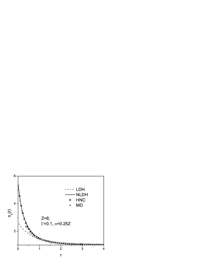
Figure 1: Electron density around an ion of charge number $Z=8$

.

II.2 Electric field time correlation function

To explore the dynamics of the electrons attention is limited to the electric field autocorrelation function defined by

$$C(t)=\frac{r_{0}^{4}}{e^{2}}<\mathbf{E}\left(t\right)\mathbf{\cdot E}>.$$ (12)

The brackets denote an equilibrium Gibbs ensemble average and $\mathbf{E}$ is the total field at the ion due to all electrons

$$\mathbf{E}=\frac{1}{Ze}\sum_{\alpha=1}^{N_{e}}\nabla_{r_{\alpha}}V_{ei}\left(r_{\alpha}\right)=\sum_{\alpha=1}^{N_{e}}\mathbf{e}\left(\mathbf{r}_{\alpha}\right)$$ (13)

$$\mathbf{e}\left(\mathbf{r}_{\alpha}\right)=e\frac{\widehat{\mathbf{r}}_{\alpha}}{r_{\alpha}^{2}}(1-(1+\frac{r_{\alpha}}{r_{0}\delta})e^{-r_{\alpha}/r_{0}\delta})$$ (14)

Consider first the initial value $C(0)$ for which two exact representations can be given

$$C(0) = \frac{r_{0}^{4}}{e^{2}}\int d\mathbf{re}\left(\mathbf{r}\right)\mathbf{\cdot}\left[n_{e}(r)\mathbf{e}\left(\mathbf{r}\right)+\int d\mathbf{r}^{\prime}n_{e}(\mathbf{r},\mathbf{r}^{\prime})\mathbf{e}\left(\mathbf{r}^{\prime}\right)\right]$$ (15)

$$= \frac{r_{0}^{4}}{e^{2}}\int d\mathbf{r}n_{e}(r)\mathbf{e}\left(\mathbf{r}\right)\mathbf{\cdot e}_{mf}\left(\mathbf{r}\right)$$

The first equality expresses the covariance in terms of both the electron density $n_{e}(r)$ and the density for two electrons near the ion $n_{e}(\mathbf{r},\mathbf{r}^{\prime})$. The second representation requires only the electron density and the mean force field derived from it

$$\mathbf{e}_{mf}\left(\mathbf{r}\right) = \frac{1}{n_{e}(r)}\left[n_{e}(r)\mathbf{e}\left(\mathbf{r}\right)+\int d\mathbf{r}^{\prime}n_{e}(\mathbf{r},\mathbf{r}^{\prime})\mathbf{e}\left(\mathbf{r}^{\prime}\right)\right]$$ (16)

$$= \frac{1}{\beta Ze}\nabla\ln\frac{n_{e}(r)}{n_{e}}.$$

The second equality is derived in Appendix A. It is similar to the first form with the apparent neglect of the two-electron ion correlations. However, these latter contributions are incorporated exactly in the mean force field $\mathbf{e}_{mf}\left(\mathbf{r}\right)$. The effects of electron-electron interactions are included in $n_{e}(r)$ through the mean field screening of the ion-electron interaction. However, $n_{e}(\mathbf{r},\mathbf{r}^{\prime})$ describes the additional electron correlations for two electrons near the ion beyond these mean field effects.

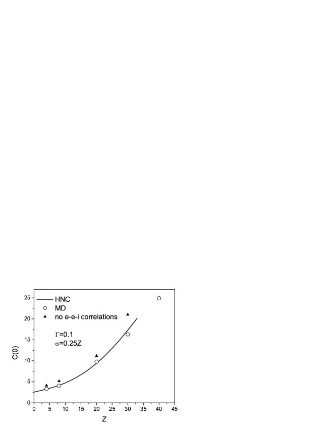
Figure 2: Initial value for the electric field autocorrelation function

.

Figure 2 shows the initial field fluctuations $C(0)$ as a function of $Z$, at $\Gamma=0.1$ and $\sigma=0.25Z$, calculated using $n_{e}(r)$ from HNC and calculated directly from MD. The solid curve is the HNC data indicating a strong $\sim Z^{3}$ dependence inherited from the electron charge density. Also shown are the results from the first equality of (15) neglecting the correlations of two electrons in the presence of the ion, $n_{e}(\mathbf{r},\mathbf{r}^{\prime})\rightarrow n_{e}(\mathbf{r})n_{e}(\mathbf{r}^{\prime})/n_{e}$. Clearly, these are significant for the conditions considered, showing the coupling between strong ion-electron interactions and weak electron-electron interactions. The results are similar for the other coupling conditions considered ($\sigma=0.5Z$ and $\sigma=2.5Z$).

It is shown in Appendix B that the time dependence of $C(t)$ in the weak coupling limit can be written as

$$C(t)=\int d\mathbf{r}d\mathbf{ve}(\mathbf{r})\cdot\mathbf{\psi}(\mathbf{r},\mathbf{v},t)$$ (17)

where $\mathbf{\psi}(\mathbf{r},\mathbf{v},t)$ obeys the linearized Vlasov equation

$$\left(\partial_{t}+\mathcal{L}\right)\mathbf{\psi}(\mathbf{r},\mathbf{v};t)=-\beta f_{e}(\mathbf{r},\mathbf{v})\mathbf{v}\cdot\mathbf{\nabla}_{\mathbf{r}}\int d\mathbf{r}_{2}V_{ee}(\mathbf{r-r}_{2})\int d\mathbf{v}_{2}\mathbf{\psi}(\mathbf{r}_{2},\mathbf{v}_{2},t).$$ (18)

The associated initial condition is

$$\mathbf{\psi}(\mathbf{r},\mathbf{v},t=0)=\mathbf{e}_{mf}(\mathbf{r})f_{e}(\mathbf{r},\mathbf{v}),$$ (19)

where $\mathbf{e}_{mf}(\mathbf{r})$ is the mean field of (16) above. The linear operator $\mathcal{L}$ is the generator for single electron dynamics in the effective potential $U_{ei}(\mathbf{r})$

$$\mathcal{L}=\mathbf{v\cdot\nabla}_{\mathbf{r}}-m_{e}^{-1}\left(\mathbf{\nabla}_{\mathbf{r}}\left(U_{ei}(\mathbf{r})\right)\right)\cdot\mathbf{\nabla}_{\mathbf{v}}.$$ (20)

The equilibrium distribution is stationary under this operator, $\mathcal{L}f_{e}(\mathbf{r},\mathbf{v})=0$. In addition to this effective single particle dynamics, all dynamical many-electron effects are contained in the term on the right side of (18). The details of the formal solution to this kinetic equation for the correlation function are given in Appendix B with the result

$$C(t)=\int_{0}^{t}dt^{\prime}\int d\mathbf{r}d\mathbf{v}f_{e}(\mathbf{r},\mathbf{v})\mathbf{e}_{s}(\mathbf{r};t^{\prime})\mathbf{e}_{mf}(\mathbf{r}(t-t^{\prime}))$$ (21)

The field $\mathbf{e}(\mathbf{r}(t-t^{\prime}))$ is given by (14) with the initial position shifted to $\mathbf{r}(t-t^{\prime})$ according to the effective single particle dynamics generated by $\mathcal{L},$ using the initial conditions $\mathbf{r},\mathbf{v}$. The other field $\mathbf{e}_{s}(\mathbf{r};t^{\prime})$ is a dynamically screened field

$$\mathbf{e}_{s}(\mathbf{r};t)=(2\pi)^{-3}\int d\mathbf{k}e^{-i\mathbf{k}\cdot r}\widetilde{\mathbf{e}}_{s}(\mathbf{k},t),\hskip 18.06749pt\widetilde{\mathbf{e}}_{s}(\mathbf{k,}t)=\int d\mathbf{k}^{\prime}\widetilde{\mathbf{e}}(\mathbf{k}^{\prime})\epsilon^{-1}\left(\mathbf{k}^{\prime},\mathbf{k},t\right)$$ (22)

where $\widetilde{\mathbf{e}}(\mathbf{k}^{\prime})$ is the Fourier transform of (14), and the dielectric function is defined by

$$\epsilon(\mathbf{k},\mathbf{k}^{\prime},t)=(2\pi)^{3}\delta(\mathbf{k}-\mathbf{k}^{\prime})+\pi(\mathbf{k,k}^{\prime},t)\widetilde{V}_{ee}(k^{\prime})$$ (23)

$$\pi(\mathbf{k,k}^{\prime},t)=\beta\frac{d}{dt}\int d\mathbf{r}d\mathbf{v}f_{e}(\mathbf{r},\mathbf{v})e^{i\mathbf{k\cdot r}}e^{-i\mathbf{k}^{\prime}\mathbf{\cdot r(}t\mathbf{)}}$$ (24)

For $Z=0$ this is the familiar classical random phase approximation for a uniform electron gas, diagonal in $\mathbf{k},\mathbf{k}^{\prime}$. More generally, the $Z$ dependence leads to a nonuniform electron density near the ion and the polarization function $\pi(\mathbf{k,k}^{\prime},t)$ depends on the details of this distribution. It vanishes at $t=0$ indicating no initial screening, $\pi(\mathbf{k,k}^{\prime},t=0)=0$. At later times the polarization function is non-zero giving a space and time dependent additional screening. Further simplification of this result for practical evaluation is discussed below.

III Molecular dynamics simulation

The application of standard MD simulation methods using the semi-classical electron-ion potential is somewhat more complex than for the usual classical fluids with short range repulsive interactions. Although finite at short distances the attractive electron-ion potential allows bound and metastable states for electrons orbiting round the ion over extended periods. For most properties, e.g., structural properties, this is not a severe problem except at low temperatures. However, the interest here is in electric field dynamics which is very sensitive to close electron-ion configurations. The protocol for control of anomalous states with quasi-bound dynamical states has been described in reference Talin and will not be repeated here.

Figure 3: Field autocorrelation function at strong coupling

.

Consider first the coupling conditions $\Gamma=0.1$ and $\sigma=0.25Z$. Figure 3 shows the field correlation function $C(t)$ for $Z=4,8,20,30,40$. There are two qualitative features to note. The first is a characteristic time for relaxation that decreases with increasing $Z$, and the second is the development of an anti-correlation that increases with increasing $Z$. Figures 4 and 5 show the corresponding results for the weaker ( $\Gamma=0.029$ and $\sigma=0.5Z$, for $Z=1,3,5,8$) and stronger ( $\Gamma=0.5$ and $\sigma=2.5Z$, for $Z=1,2,3,4,6,10$) coupling cases. In the former case the decreasing relaxation time is evident but the anti-correlation is significant only for the $Z=8$ curve. The strongest coupling case of Fig. 5 shows large anti-correlation for all $Z$. It should be noted that this last case is unrealistic since the equilibrium population of ions at such strong coupling is extremely small.

Figure 4: Field autocorrelation function at moderate coupling

.

Figure 5: Field autocorreltion function at very strong coupling

.

Figure 6: Time integral of $C(t)$ as a function of $Z$ for moderate, strong, and very strong coupling cases

.

Figure 7: Same as Fig. 6 as a function of $\sigma$

.

The area under the curves is related to transport properties, as indicated in the next section, and results from a competition between these two features and the increasing initial correlations. The effects of shortening decay time and anti-correlation dominate to decrease the area as indicated in Fig. 6. These effects are greater for stronger coupling, with significant anti-correlation occurring for $Z\geq 4$. Figure 7 shows the same results plotted as a function of $\sigma$. The three cases appear similar, with only a shift in their $\sigma=0$ value due to different values for $\gamma$ and $\delta$. This suggests that the time integral of the correlation function, normalized to its value at $\sigma=0$ may be a ”universal” function of sigma.

IV Effective single particle model

To calculate the correlation function and identify the mechanisms for the decay time and correlation, it might be supposed that the single nearest electron dominates since its field is greatest. Figure 8 shows this nearest neighbor contribution from MD for the same conditions of Fig. 3.

Figure 8: Nearest neighbor field autocorrelation function for strong coupling

.

Clearly, the nearest neighbor field autocorrelation function has the same qualitative behavior as the total correlation function with respect to the decreasing decay time and increasing anti-correlation. The quantitative values are wrong (both amplitude and time scale), however, suggesting that contributions from other particles are important as well. To explore this in more detail, the Vlasov equation given by (21) can be used. It requires evaluation of the dynamically screened field $\mathbf{e}_{s}(\mathbf{r};t)$, although at short times $\mathbf{e}_{s}(\mathbf{r};t)\sim\mathbf{e}(\mathbf{r};0)=\mathbf{e}(\mathbf{r})$. The correlation function is then effectively that for a single particle moving in the self-consistent potential (10), averaged over the initial equilibrium distribution of electrons about the ion. Thus it is similar to the nearest neighbor approximation but extends it to include all electrons, including the correct initial correlations and the correlations of the mean field for the dynamics. If the additional dynamical screening is neglected for all relevant times, i.e.

$$\mathbf{e}_{s}(\mathbf{r};t)\rightarrow\delta(t)\mathbf{e}(\mathbf{r})$$ (25)

then (21) becomes

$$C(t)\rightarrow\int d\mathbf{r}d\mathbf{v}f_{e}(\mathbf{r},\mathbf{v})\mathbf{e}(\mathbf{r})\mathbf{e}_{mf}(\mathbf{r}(t)).$$ (26)

Comparison with (15) shows that this approximation is exact for $C(0)$. For practical purposed, this approximation for $C(t)$ has been evaluated using the analytic nonlinear Debye form (11) fitted to the HNC results in both the dynamics and the electron density. The results for this effective single particle model are shown in Figs. 9 and 10 for the case $\Gamma=0.1$ and $\sigma=0.25Z$.

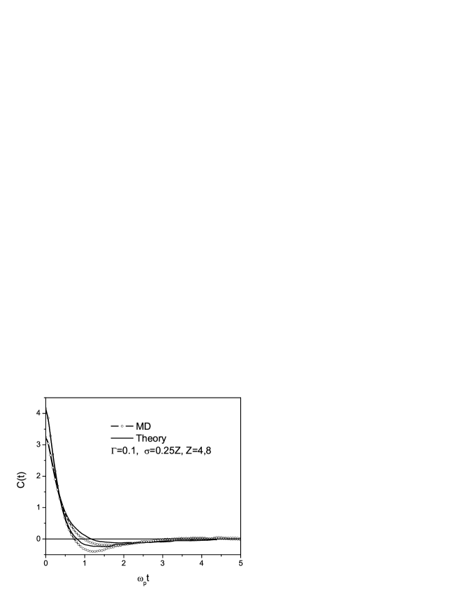
Figure 9: Comparison of $C(t)$ from MD with results from mean field kinetic theory for $Z=4,8$

.

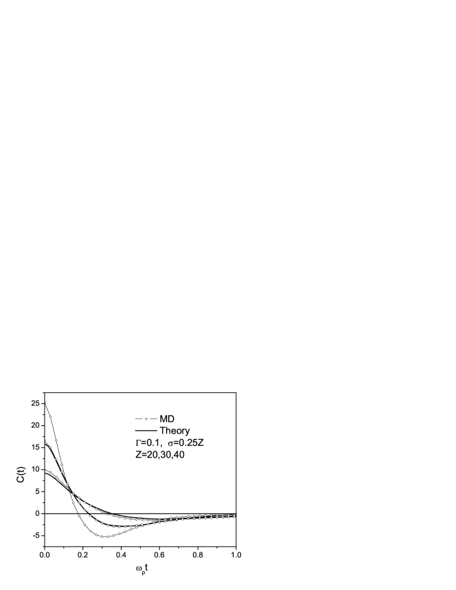
Figure 10: Same as Figure 9 for $Z=20,30$

.

The agreement between this simple theory is quite good and provides a means to interpret the results of the MD simulation. The initial position and velocity of an electron are sampled from the equilibrium distribution $f_{e}(\mathbf{r},\mathbf{v})$ which favors electrons close to the ion and hence large fields. Since the force on the electron is also large, its initial acceleration will be large. This is the source of the short decay time. Consider the case of an energetic electron near the ion. If its velocity is directed away from the ion it will move to larger distances and the field will decrease with a positive component along the initial field. In contrast, if its initial velocity is toward the ion it will move past the ion with a change in the direction of its field relative to the initial value. This is a source for anti-correlation. For less energetic electrons, the trajectories are bound and there is continual correlation and anti-correlation as the correlation function decays in magnitude due to phase averaging. Both the increase in initial correlation and the field reversal effects should increase as the charge on the ion increases, and this is what is observed. At weaker electron-ion coupling both effects are diminished and blurred as the relevant configurations are more distant, the fields are weaker, and the accelerations smaller. This is already evident in the nearest neighbor results of Fig. 8.

The simple model of (26) appears better at larger values of $Z$ where the single particle motion is expected to dominate. For smaller values of $Z$ the agreement at short times is still good (the discrepancy at $t=0$ is a limitation of HNC, not the dynamics), but more significant differences occur after the first initial decrease. Presumably, this is due to the dynamical screening effects in $\mathbf{e}_{s}(\mathbf{r};t)$ that have been neglected. It should be noted that the results here are somewhat sensitive to the choice of parameters $\overline{Z}$, $\overline{\lambda}$ used in fitting the non-linear Debye Huckel form for $f_{e}(\mathbf{r},\mathbf{v})$. Fits emphasizing short or intermediate distances change slightly the point at which anti-correlation sets in and its amplitude. The primary criterion used here was a globally good visual fit and a good resulting value for the initial condition $C(0)$.

V Stopping power, friction, and self-diffusion

Emphasis here has been placed on the electric field autocorrelation function as a sensitive measure of electron properties near the ion. This function is also of interest because of its connection to transport and radiative properties of the ion. Specifically, for the case of an infinitely massive ion considered here there are exact relationships between transport coefficients characterizing three physically different phenomena: 1) the low velocity stopping power $\mathcal{S}$ for a particle injected in the electron gas, 2) the friction coefficient $\xi$ for the resistance to a particle being pulled through the gas, and 3) the self-diffusion coefficient $D$ of a particle at equilibrium with the gas Berkovsky3

$$m_{0}\xi=\left(\beta D\right)^{-1}=\frac{\mathcal{S}(v)}{v}\mid_{v=0}=\beta Z^{2}r_{0}^{-4}\int_{0}^{\infty}dtC(t)$$ (27)

Finally, the time integral of $C(t)$ also provides the fast fluctuation limit (impact) for the spectral line width of ions broadened by electrons lineshape . Clearly, a better understanding of the mechanisms controlling the electric field autocorrelation function is of interest in several different contexts.

This Green-Kubo representation (27) allows a determination of these transport properties from an equilibrium MD simulation, as described above. In contrast, previous simulations of stopping power have studied the nonequilibrium state of the injected particle, measuring directly the energy degradation Zwick . At asymptotically weak coupling, these properties have a dominant $Z^{2}$ dependence, as $C(t)$ becomes independent of $Z$. A puzzling result of the previous simulations Zwick , and some experiments Experiment , was the observation of a weaker $Z$ dependence at strong coupling. This behavior is somewhat puzzling in light of the strong growth of the initial value $C(0)\approx Z^{3}$ at large $Z$ (see Fig. 2). Thus it would appear that the dominant dependence would be an even stronger $Z^{5}$. However, as Fig. 6 shows clearly the competing effects of decreasing correlation time and a developing time interval of anti-correlation dominate at strong coupling to decrease the time integral.

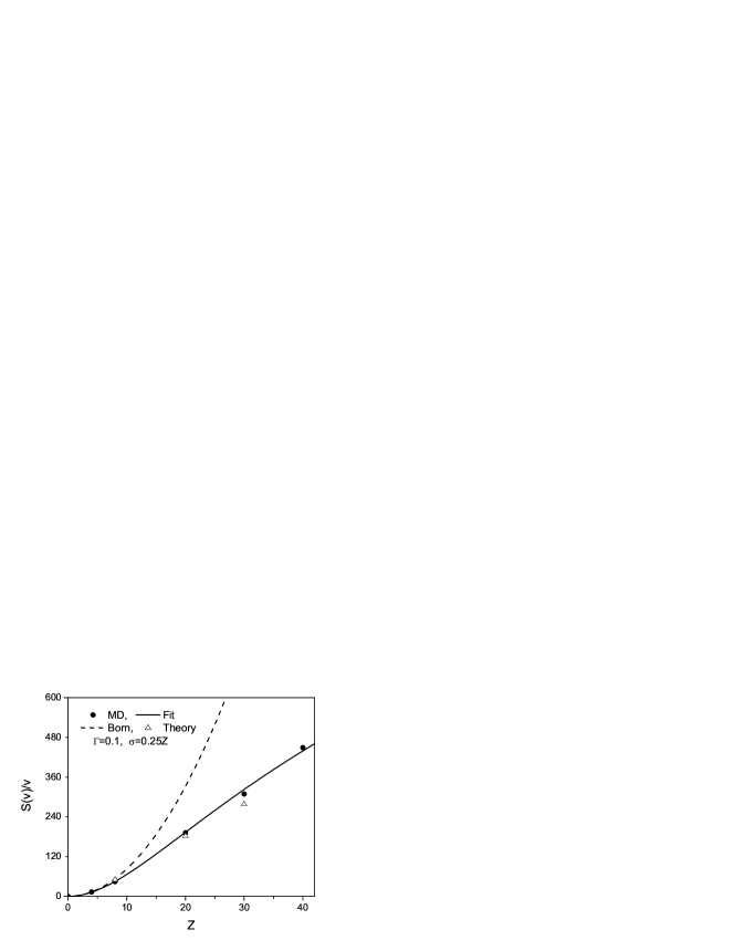
Figure 11: Stopping power relative to the speed at zero speed, Eq. (27), at strong coupling. Also shown is the Born approximation and the results of the kinetic theory

.

Figure 11 shows the dimensionless stopping power as a function of $Z$ for the case $\Gamma=0.1$ and $\sigma=0.25Z$. Also shown is the Born approximation $0.83Z^{2}$, where the coefficient has been determined by the data for small $Z$. The MD data has been fit to a crossover function

$$\frac{\mathcal{S}(v)}{v}\mid_{v=0}\rightarrow\frac{0.83Z^{2}}{1+0.008Z^{1/2}}.$$ (28)

This form has been chosen since it implies the stopping power goes as $Z^{3/2}$ at extreme coupling, which is consistent with the earlier results Zwick ; Experiment . However, other fits to the data here are possible as well. The predictions of the simple effective single particle theory are shown on Fig. 11 also.

Figure 12: Same as Fig. 11 at moderate coupling

.

Figure 13: Same as Fig. 11 at very strong coupling

.

Similar results are obtained for the other coupling cases. Figure 12 shows the stopping power for the weaker coupling case of $\Gamma=0.029$ and $\sigma=0.5Z$ at smaller values of $Z$. The Born approximation $1.88Z^{2}$ is determined by the $Z=1$ value. As expected the Born approximation is quite good at weak coupling, although some deviation is seen at $Z=8$. This is consistent with the above estimate that strong coupling effects in Fig. 6 occur for $\sigma\geq 4.$ The strongest coupling case of $\Gamma=0.5$ and $\sigma=2.5Z$ is shown in Fig. 13, where the Born approximation is again determined from the $Z=1$ data and found to be $1.52Z^{2}$. The deviations from the Born approximation are much greater now, as expected.

VI Summary and Discussion

The objective here has been to explore the dynamics of electrons near a positive ion as a function of the charge number on the ion, or more precisely, as a function of the electron-ion coupling $\sigma=Z\Gamma/\delta$. A primary tool for this investigation has been molecular dynamics simulation, requiring a semi-classical regularization of the Coulomb potential at short distances. Under the hot, dense conditions needed to support large $Z$ ions the electron coupling can be quite weak. An accurate theoretical description is then given by the nonlinear Vlasov kinetic equation for the electrons. The MD simulation reveals an interesting structure for the electric field autocorrelation function. At the weakest coupling considered there is a rapid initial decay followed by an asymptotic domain of weak anticorrelation. The time scale for the initial decay decreases with increasing $Z$ but does not depend strongly on $Z$ as long as the coupling stays weak. This is illustrated in Fig. 4. Figures 5 and 6 show a quite different behavior at strong coupling where the initial decay time shortens and the anticorrelation becomes prominent on the same time scale. This qualitative behavior is characteristic of the single electron dynamics of the nearest neighbor. A quantitative description is provided by the Vlasov kinetic theory with the exact initial condition for the distribution of electrons about the ion, including strong electron-ion correlations mediated by weak electron-electron interactions. The mean field dynamics is that of effective single electron trajectories, calculated for the same effective potential as that for the initial correlations, and averaged over an ensemble of these initial states.

The simple theoretical model provides a means to interpret the MD simulation data for the beginnings of a phenomenological understanding of electron dynamics near a positive ion. The initial correlation for the electric field $C(0)$ increases with $Z$ as the equilibrium distribution of electrons is enhanced near the ion with configurations corresponding to larger fields. The latter is well described by the nonlinear Debye-Huckel form given by (9) with (11). The initial decay of $C(t)$ is essentially the decorrelation time for a ”most probable” electron near the ion. This most probable distance can be estimated from the maximum of the Debye distribution $P(r)=4\pi r^{2}n_{e}(r)/n_{e}$ $\equiv 4\pi r^{2}e^{-\beta U_{ei}(r)}$ to give $r/r_{0}\sim\delta$ for strong coupling. The correlation time is then approximately the time to accelerate this electron to the position of the ion, $t_{c}\sim\left(r_{0}\delta/\sqrt{\beta m}\right)\sqrt{1/Z\Gamma}$. The first factor $r_{0}\delta/\sqrt{\beta m}$ is the time for an electron with the thermal velocity to cross a sphere of the size of the thermal de Broglie diameter. The second factor gives the dominant $Z$ dependence $t_{c}\sim\sqrt{1/Z}$. As the electron continues past the ion its acceleration changes sign as it is attracted to the ion with a field opposite that of the original field. This is the source of the dominant anticorrelation.

The self-diffusion coefficient, stopping power, friction coefficient, and width of spectral lines are proportional to the integral of $C(t)$. At $Z=0$ this is the field autocorrelation function at a neutral point and is independent of $Z$, depending only on the electron-electron coupling. As $Z$ increases the electron distribution becomes nonuniform about the ion and $C(0)$ increases. At the same time $t_{c}$ decreases. For small $Z$ these two effects become negligible, as seen in Fig. 6 for the case of $\sigma=0.5Z$ and $Z<5$. As $Z$ increases, or more precisely as $\sigma$ increases, the domain of anticorrelation appears and begins to dominate the decrease in the integral of $C(t)$. These basic mechanisms are captured by the meanfield description based on the Vlasov equation for the one particle electron distribution. The relevant correlations contained in this description are those of the equilibrium electron distribution about the ion, also described well by the stationary solution to the Vlasov equation.

This analysis provides a new picture for the puzzling decrease of stopping power with increasing $Z$, relative to the Born approximation. The stopping power is proportional to $Z^{2}$ times the time integral of $C(t)$ which is essentially the total cross section for all the electrons and the ion. The decrease towards a $Z^{3/2}$ dependence at strong coupling observed earlier is seen to be due to the effects just described. However, the precise dependence on $Z$ may be more complicated as the coupling increases.

Similarly, these same results provide clear evidence for the effects of electron-electron and electron-ion correlations on the shape of spectral lines Talin2 ; Talin3 . Similar experimental puzzles regarding the $Z$ dependence of the half width 3s3p can be clarified through combined theoretical and MD simulation as described here.

VII Acknowledgments

Support for this research has been provided by the U.S. Department of Energy Grant No. DE-FG03-98DP00218. The authors thank M. Gigosos for helpful discussions and suggestions. J. Dufty is grateful for the support and hospitality of the University of Provence.

Appendix A Evaluation of the field covariance

The dimensionless electric field covariance is defined by

$$C(0)=\frac{r_{0}^{4}}{e^{2}}<\mathbf{E}\cdot\mathbf{E}>$$ (29)

with

$$\mathbf{E}=\sum_{\alpha=1}^{N_{e}}\mathbf{e}\left(\mathbf{r}_{\alpha}-\mathbf{r}_{0}\right).$$ (30)

Here $\mathbf{r}_{0}$ denotes the position of the ion. The equilibrium average can be calculated directly in terms of the one and two electron charge densities

$$C(0)=\frac{r_{0}^{4}}{e^{2}}\int d\mathbf{re}\left(\mathbf{r}\right)\mathbf{\cdot}\left[n_{e}(r)\mathbf{e}\left(\mathbf{r}\right)+\int d\mathbf{r}^{\prime}n_{e}(\mathbf{r},\mathbf{r}^{\prime})\mathbf{e}\left(\mathbf{r}^{\prime}\right)\right]$$ (31)

with the definitions

$$n_{e}(r_{1})=N\frac{\int d\mathbf{r}_{0}d\mathbf{r}_{2}..d\mathbf{r}_{N}e^{-\beta U}}{\int d\mathbf{r}_{0}..d\mathbf{r}_{N}e^{-\beta U}},\hskip 18.06749ptn_{e}(\mathbf{r}_{1},\mathbf{r}_{2})=N(N-1)\frac{\int d\mathbf{r}_{0}d\mathbf{r}_{3}..d\mathbf{r}_{N}e^{-\beta U}}{\int d\mathbf{r}_{0}..d\mathbf{r}_{N}e^{-\beta U}},$$ (32)

where $U$ is the total kinetic energy and $T=1/k_{B}\beta$ is the temperature.

An equivalent alternative form is obtained by writing the covariance as

$$C(0) = -\frac{r_{0}^{4}}{Ze^{3}}<\nabla_{r_{0}}U_{ie}\cdot\mathbf{E}>=\frac{r_{0}^{4}}{\beta Ze^{3}}\frac{\int d\mathbf{r}_{0}d\mathbf{r}_{2}..d\mathbf{r}_{N}\left(\nabla_{r_{0}}e^{-\beta U}\right)\cdot\mathbf{E}}{\int d\mathbf{r}_{0}..d\mathbf{r}_{N}e^{-\beta U}}$$ (33)

$$= \frac{r_{0}^{4}}{\beta Ze^{3}}\left\langle\nabla_{r_{0}}\cdot\mathbf{E}\right\rangle=-\frac{r_{0}^{4}}{\beta Ze^{3}}\int d\mathbf{r}n_{e}(r)\nabla\mathbf{\cdot e}\left(\mathbf{r}\right)$$

$$= \frac{r_{0}^{4}}{\beta Ze^{3}}\int d\mathbf{r}n_{e}(r)\left(\frac{1}{\beta Ze}\nabla\ln n_{e}(r)\right)\mathbf{\cdot e}\left(\mathbf{r}\right)=\frac{r_{0}^{4}}{e^{2}}\int d\mathbf{r}n_{e}(r)\mathbf{e}_{mf}\left(\mathbf{r}\right)\mathbf{\cdot e}\left(\mathbf{r}\right)$$

In the last equality the mean force field has been introduced by

$$\mathbf{e}_{mf}\left(\mathbf{r}\right)=\frac{1}{\beta Ze}\nabla\ln n_{e}(r,t).$$ (34)

Finally, comparison of (31) and (33) gives the alternative expression for this field

$$\mathbf{e}_{mf}\left(\mathbf{r}\right)=\frac{1}{n_{e}(r)}\left[n_{e}(r)\mathbf{e}\left(\mathbf{r}\right)+\int d\mathbf{r}^{\prime}n_{e}(\mathbf{r},\mathbf{r}^{\prime})\mathbf{e}\left(\mathbf{r}^{\prime}\right)\right].$$ (35)

Appendix B Kinetic equation for correlation functions

In this section the evaluation of the field autocorrelation function by kinetic theory, and the basis for the approximation (18), are briefly described. First, the correlation function is formally rewritten as

$$C(t) = \frac{r_{0}^{4}}{e^{2}}<\mathbf{E}\left(t\right)\mathbf{\cdot E}>=\frac{r_{0}^{4}}{e^{2}}\int d\mathbf{r}_{1}d\mathbf{v}_{1}\mathbf{..}d\mathbf{r}_{N}d\mathbf{v}_{N}\mathbf{E\cdot E}\left(-t\right)\rho_{e}$$ (36)

$$= \frac{r_{0}^{4}}{e^{2}}\int d\mathbf{r}_{1}d\mathbf{v}_{1}\mathbf{e}\left(\mathbf{r}_{1}\right)N\mathbf{\cdot}\int d\mathbf{r}_{2}d\mathbf{v}_{2}\mathbf{..}d\mathbf{r}_{N}d\mathbf{v}_{N}\mathbf{E}\left(-t\right)\rho_{e}$$

$$= \frac{r_{0}^{4}}{e^{2}}\int d\mathbf{r}_{1}d\mathbf{v}_{1}\mathbf{e}\left(\mathbf{r}_{1}\right)\cdot\mathbf{\psi}(\mathbf{r}_{1},\mathbf{v}_{1};t)$$

where $\rho_{e}$ is the equilibrium Gibbs ensemble and $\mathbf{e}\left(\mathbf{r}_{\alpha}\right)$ is the single particle field of (18). The integrations over degrees of freedom $2..N$ in the second equality define a reduced function $\mathbf{\psi}(\mathbf{r}_{1},\mathbf{v}_{1};t)$ which is the first member of a set of such functions

$$\mathbf{\psi}^{(s)}(\mathbf{r}_{1},\mathbf{v}_{1};..\mathbf{r}_{s},\mathbf{v}_{s};t)=N^{s}\int d\mathbf{r}_{s+1}d\mathbf{v}_{s+1}\mathbf{..}d\mathbf{r}_{N}d\mathbf{v}_{N}\mathbf{E}\left(-t\right)\rho_{e}.$$ (37)

It is straightforward to verify that these functions satisfy the BBGKY hierarchy, whose first equation is formally the same as (4)

$$\left(\partial_{t}+\mathbf{v\cdot\nabla}_{\mathbf{r}}-m_{e}^{-1}\left(\mathbf{\nabla}_{\mathbf{r}}\left(V_{ei}(\mathbf{r})+V_{eb}(\mathbf{r})\right)\right)\cdot\mathbf{\nabla}_{\mathbf{v}}\right)\mathbf{\psi}(\mathbf{r}_{1},\mathbf{v}_{1};t)$$ (38)

$$= m_{e}^{-1}\int d\mathbf{r}_{2}d\mathbf{v}_{2}\left(\mathbf{\nabla}_{\mathbf{r}}V_{ee}(\mathbf{r-r}_{2})\right)\cdot\mathbf{\nabla}_{\mathbf{v}}\mathbf{\psi}^{(2)}(\mathbf{r},\mathbf{v};\mathbf{r}_{2},\mathbf{v}_{2};t).$$

However, in contrast to the distribution functions in (4) the functional relationship of $\mathbf{\psi}^{(2)}$ to $\mathbf{\psi}$ is linear. To see this, consider first the initial conditions which are found to be

$$\mathbf{\psi}(\mathbf{r}_{1},\mathbf{v}_{1};t = 0)=f_{e}(\mathbf{r}_{1},\mathbf{v}_{1})\mathbf{e}\left(\mathbf{r}_{1}\right)+\int d\mathbf{r}_{2}d\mathbf{v}_{2}f_{e}^{(2)}(\mathbf{r}_{1},\mathbf{v}_{1};\mathbf{r}_{2},\mathbf{v}_{2})\mathbf{e}\left(\mathbf{r}_{2}\right)$$ (39)

$$= f_{e}(\mathbf{r}_{1},\mathbf{v}_{1})\mathbf{e}_{mf}(\mathbf{r}_{1})$$

$$\mathbf{\psi}^{(2)}(\mathbf{r}_{1},\mathbf{v}_{1};\mathbf{r}_{2},\mathbf{v}_{2};t = 0)=f_{e}^{(2)}(\mathbf{r}_{1},\mathbf{v}_{1};\mathbf{r}_{2},\mathbf{v}_{2})\left(\mathbf{e}\left(\mathbf{r}_{1}\right)+\mathbf{e}\left(\mathbf{r}_{2}\right)\right)$$

$$+n\int d\mathbf{r}_{3}d\mathbf{v}_{3}f_{e}^{(3)}(\mathbf{r}_{1},\mathbf{v}_{1};\mathbf{r}_{2},\mathbf{v}_{2};\mathbf{r}_{3},\mathbf{v}_{3})\mathbf{e}\left(\mathbf{r}_{3}\right)$$

$$= f_{e}^{(2)}(\mathbf{r}_{1},\mathbf{v}_{1};\mathbf{r}_{2},\mathbf{v}_{2})\left(\mathbf{e}_{m}\left(\mathbf{r}_{1}\right)+\mathbf{e}_{m}\left(\mathbf{r}_{2}\right)\right)$$ (40)

$$+n\int d\mathbf{r}_{3}d\mathbf{v}_{3}h_{e}^{(3)}(\mathbf{r}_{1},\mathbf{v}_{1};\mathbf{r}_{2},\mathbf{v}_{2};\mathbf{r}_{3},\mathbf{v}_{3})\mathbf{e}\left(\mathbf{r}_{3}\right)$$

Here, $f_{e}^{(s)}$ are the equilibrium $s-$particle reduced distribution functions associated with the Gibbs ensemble and $h_{e}^{(3)}$ is the equilibrium correlation function for three electrons in the presence of the ion

$$h_{e}^{(3)}(\mathbf{r}_{1},\mathbf{v}_{1};\mathbf{r}_{2},\mathbf{v}_{2};\mathbf{r}_{3},\mathbf{v}_{3};t) = f_{e}^{(3)}(\mathbf{r}_{1},\mathbf{v}_{1};\mathbf{r}_{2},\mathbf{v}_{2};\mathbf{r}_{3},\mathbf{v}_{3})$$ (41)

$$-f_{e}^{(2)}(\mathbf{r}_{1},\mathbf{v}_{1};\mathbf{r}_{2},\mathbf{v}_{2})\frac{1}{f_{e}(\mathbf{r}_{1},\mathbf{v}_{1})}f_{e}^{(2)}(\mathbf{r}_{1},\mathbf{v}_{1};\mathbf{r}_{3},\mathbf{v}_{3})$$

$$-f_{e}^{(2)}(\mathbf{r}_{1},\mathbf{v}_{1};\mathbf{r}_{2},\mathbf{v}_{2})\frac{1}{f_{e}(\mathbf{r}_{2},\mathbf{v}_{2})}f_{e}^{(2)}(\mathbf{r}_{2},\mathbf{v}_{2};\mathbf{r}_{3},\mathbf{v}_{3})$$

The linear functional relationship between $\mathbf{\psi}^{(2)}$ to $\mathbf{\psi}$ at $t=0$ is now evident

$$\mathbf{\psi}^{(2)}(\mathbf{r}_{1},\mathbf{v}_{1};\mathbf{r}_{2},\mathbf{v}_{2};0) = f_{e}^{(2)}(\mathbf{r}_{1},\mathbf{v}_{1};\mathbf{r}_{2},\mathbf{v}_{2};t)\left(\frac{\mathbf{\psi}(\mathbf{r}_{1},\mathbf{v}_{1};0)}{f_{e}(\mathbf{r}_{1},\mathbf{v}_{1})}+\frac{\mathbf{\psi}(\mathbf{r}_{2},\mathbf{v}_{2};0)}{f_{e}(\mathbf{r}_{2},\mathbf{v}_{2})}\right)$$ (42)

$$+3\text{ electron correlations.}$$

Recognizing this linear relationship, the basic approximation for weak coupling among the electrons is to neglect all of their correlations at all times, i.e. extend (42) to

$$\mathbf{\psi}^{(2)}(\mathbf{r}_{1},\mathbf{v}_{1};\mathbf{r}_{2},\mathbf{v}_{2};t)\rightarrow f_{e}(\mathbf{r}_{2},\mathbf{v}_{2};t)\mathbf{\psi}(\mathbf{r}_{1},\mathbf{v}_{1};t)+f_{e}(\mathbf{r}_{1},\mathbf{v}_{1};t)\mathbf{\psi}(\mathbf{r}_{2},\mathbf{v}_{2};t).$$ (43)

Use of this in the first hierarchy equation (38) gives directly the kinetic equation (18) discussed in the text

$$\left(\partial_{t}+\mathcal{L}\right)\mathbf{\psi}(\mathbf{r},\mathbf{v};t)=-\beta f_{e}(\mathbf{r},\mathbf{v})\mathbf{v}\cdot\mathbf{\nabla}_{\mathbf{r}}\int d\mathbf{r}_{2}V_{ee}(\mathbf{r-r}_{2})\int d\mathbf{v}_{2}\mathbf{\psi}(\mathbf{r}_{2},\mathbf{v}_{2},t).$$ (44)

$$\mathcal{L}=\mathbf{v\cdot\nabla}_{\mathbf{r}}-m_{e}^{-1}\left(\mathbf{\nabla}_{\mathbf{r}}\left(U_{ei}(\mathbf{r})\right)\right)\cdot\mathbf{\nabla}_{\mathbf{v}}.$$ (45)

Appendix C Solution to kinetic equation

The operator $\mathcal{L}$ in (38) is the generator for single electron dynamics in the effective potential due to the ion $U_{ei}(\mathbf{r})$. The solution to the equation can be obtained in terms of this single electron dynamics by direct integration

$$\mathbf{\psi}(\mathbf{r},\mathbf{v};t)=e^{-\mathcal{L}t}\mathbf{\psi}(\mathbf{r},\mathbf{v};0)-\int_{0}^{t}d\tau e^{-\mathcal{L}\left(t-\tau\right)}f_{e}(\mathbf{r},\mathbf{v})\beta\mathbf{v}\cdot\mathbf{\nabla}_{\mathbf{r}}\int d\mathbf{r}_{2}V_{ee}(\mathbf{r-r}_{2})\mathbf{I}(\mathbf{r}_{2},\tau)$$ (46)

$$\mathbf{I}(\mathbf{r},t)=\int d\mathbf{v\psi}(\mathbf{r},\mathbf{v},t)$$ (47)

The initial condition is given by (39). An equation for $\mathbf{I}(\mathbf{r},t)$ follows from substitution of (46) into (47)

$$\mathbf{I}(\mathbf{r};t)=\int d\mathbf{v}e^{-\mathcal{L}t}f_{e}(\mathbf{r},\mathbf{v})\mathbf{e}_{mf}(\mathbf{r})-\int_{0}^{t}d\tau\int d\mathbf{v}e^{-\mathcal{L}\left(t-\tau\right)}f_{e}(\mathbf{r},\mathbf{v})\beta\mathbf{v}\cdot\mathbf{\nabla}_{\mathbf{r}}\int d\mathbf{r}_{2}V_{ee}(\mathbf{r-r}_{2})\mathbf{I}(\mathbf{r}_{2},\tau).$$ (48)

This is an integral equation for $\mathbf{I}(\mathbf{r};t)$ which can be written

$$\int_{0}^{t}d\tau\int d\mathbf{r}_{2}\epsilon\left(\mathbf{r},t;\mathbf{r}_{2},\tau\right)\mathbf{I}(\mathbf{r}_{2};\tau)=\int d\mathbf{v}e^{-\mathcal{L}t}f_{e}(\mathbf{r},\mathbf{v})\mathbf{e}_{mf}(\mathbf{r}).$$ (49)

The dielectric function $\epsilon\left(\mathbf{r},t-\tau;\mathbf{r}_{2}\right)$ is defined by

$$\epsilon\left(\mathbf{r},t-\tau;\mathbf{r}^{\prime}\right)=\delta\left(t-\tau\right)\delta\left(\mathbf{r}-\mathbf{r}^{\prime}\right)+\int d\mathbf{r}^{\prime\prime}\pi\left(\mathbf{r},t-\tau;\mathbf{r}^{\prime\prime}\right)V_{ee}(\mathbf{r}^{\prime\prime}\mathbf{-r}^{\prime}),$$ (50)

where the polarization function is

$$\pi\left(\mathbf{r},t;\mathbf{r}^{\prime}\right)=\int d\mathbf{v}e^{-\mathcal{L}t}f_{e}(\mathbf{r},\mathbf{v})\beta\mathbf{v}\cdot\mathbf{\nabla}_{\mathbf{r}}\delta\left(\mathbf{r}-\mathbf{r}^{\prime}\right).$$ (51)

With these results the correlation function from (36) becomes

$$C(t) = \frac{r_{0}^{4}}{e^{2}}\int d\mathbf{r}d\mathbf{ve}\left(\mathbf{r}\right)\cdot\mathbf{\psi}(\mathbf{r},\mathbf{v};t)=\frac{r_{0}^{4}}{e^{2}}\int d\mathbf{re}\left(\mathbf{r}\right)\cdot\mathbf{I}(\mathbf{r};t)$$ (52)

$$= \frac{r_{0}^{4}}{e^{2}}\int_{0}^{t}d\tau\int d\mathbf{re}\left(\mathbf{r}\right)\cdot\int d\mathbf{r}_{2}\epsilon^{-1}\left(\mathbf{r},\tau;\mathbf{r}_{2},\right)\int d\mathbf{v}e^{-\mathcal{L}\left(t-\tau\right)}f_{e}(\mathbf{r}_{2},\mathbf{v})\mathbf{e}_{mf}(\mathbf{r}_{2})$$

$$= \frac{r_{0}^{4}}{e^{2}}\int_{0}^{t}d\tau\int d\mathbf{r}d\mathbf{\mathbf{v}e}_{s}\left(\mathbf{r},\tau\right)\cdot e^{-\mathcal{L}\left(t-\tau\right)}f_{e}(\mathbf{r},\mathbf{v})\mathbf{e}_{mf}(\mathbf{r}).$$

In the last equality the screened field $\mathbf{e}_{s}\left(\mathbf{r},t\right)$ has been introduced

$$\mathbf{e}_{s}\left(\mathbf{r},t\right)\equiv\int d\mathbf{r}^{\prime}\mathbf{e}\left(\mathbf{r}^{\prime}\right)\epsilon^{-1}\left(\mathbf{r}^{\prime},t;\mathbf{r}\right)$$ (53)

Finally, using the stationarity of $f_{e}(\mathbf{r},\mathbf{v})$ under the dynamics generated by $\mathcal{L}$ gives

$$C(t) = \frac{r_{0}^{4}}{e^{2}}\int_{0}^{t}d\tau\int d\mathbf{r}d\mathbf{\mathbf{v}}f_{e}\mathbf{(\mathbf{r},\mathbf{v})e}_{s}\left(\mathbf{r},\tau\right)\cdot e^{-\mathcal{L}\left(t-\tau\right)}\mathbf{e}_{mf}(\mathbf{r})$$ (54)

$$\equiv \frac{r_{0}^{4}}{e^{2}}\int_{0}^{t}d\tau\int d\mathbf{r}d\mathbf{\mathbf{v}}f_{e}\mathbf{(\mathbf{r},\mathbf{v})e}_{s}\left(\mathbf{r},\tau\right)\cdot\mathbf{e}_{mf}(\mathbf{r}\left(t-\tau\right)).$$

This is the form used in the text, Eq. (21).

References

- (1) J. W. Dufty in Strongly Coupled Plasmas, 493, de Witt H and Rogers F editors (NATO ASI Series, Plenum, NY, 1987).
- (2) M. Berkovsky, J.W. Dufty, A. Calisti, R. Stamm, and B. Talin, Phys. Rev. E 51, 4917 (1995).
- (3) J. W. Dufty and L. Zogaib in Strongly Coupled Plasma Physics, 533, S. Ichimaru, ed. (Elsevier Pub. B. V. Yamada Science Foundation, 1990); J. W. Dufty and L. Zogaib, Phys. Rev. A 44, 2612 (1991); J. W. Dufty, in Physics of Non-ideal Plasmas-selected papers, 215, W. Ebeling, A. Forster, and R. Radtke eds. (Teubner-Texte vol. 26, Stuttgart, 1992); J. W. Dufty and L. Zogaib, Phys. Rev. E 47, 2958 (1993).
- (4) A. Alastuey, J.L. Lebowitz, and D. Levesque, Phys. Rev. A 43, 2673 (1991).
- (5) D.B. Boercker, C.A. Iglesias, and J. W. Dufty, Phys. Rev. A 36, 2254 (1987).
- (6) M.A. Berkovsky, J. W. Dufty, A. Calisti, R. Stamm, and B. Talin, Phys. Rev. E 54, 4087 (1996).
- (7) B. Talin, A. Calisti and J. Dufty, Phys. Rev. E 65, 056406 (2002).
- (8) B. Talin and J. W. Dufty, Contrib. Plasma Phys. 41 , 195 (2001); B. Talin, A. Calisti, and J. W. Dufty, Contrib. Plasma Phys. 41, 195 (2001).
- (9) A. Filinov, M. Bonitz, and W. Ebeling, J. Phys. A 36, 5957 (2003); A. Filinov, V. Golubnychiy, M. Bonitz, W. Ebeling, and J. W. Dufty, ”Improved quantum pair potentials for correlated Coulomb systems”, preprint.
- (10) T. Pschiwul and G. Zwicknagel, J. Phys. A 36, 6251 (2003); Contrib. Plasma Phys. 41, 271 (2001).
- (11) G. Norman, A. Valuev, and I. Valuev, J. Phys. IV France 10, Pr5-255 (2000); W. Ebeling, G. Norman, A. Valuev, and I. Valuev, Contrib. Plasma Phys. 39, 61 (1999); J. Ortner, I. Valuev, and W. Ebeling, Contrib. Plasma Phys. 39, 311 (1999).
- (12) J-P Hansen and I. MacDonald, Theory of Simple Liquids, (Academic Press, San Diego, 1990).
- (13) L. Zogaib and J. Dufty, ”The semi-classical form of DFT for a quantum plasma”, preprint.
- (14) J. W. Dufty and M. Berkovsky, Nucl. Inst. Meth. B 96, 626 (1995).
- (15) J. W. Dufty and M. Berkovsky in Physics of Strongly Coupled Plasmas edited by Kraeft W, Schlanges M, Haberland H and Bornath T (World Scientific, River Edge, NJ, 1996).
- (16) H. Minoo, M.M. Gombert and C. Deutsch Phys. Rev. A 23, 924 (1981)
- (17) J. A. McLennan, Introduction to Nonequilibrium Statistical Mechanics, (Prentice-Hall, New Jersey, 1989).
- (18) M. Lewis, Phys. Rev. 121, 501 (1964); C. Cohen-Tannoudji, Aux Frontières de la Spectroscopie Laser, Vol. 1, North-Holland Publishing Company 1975)
- (19) G. Zwicknagel, C. Toepffer and P-G. Reinhard, Physics Reports 309, 118 (1999)
- (20) Th. Winkler et al., Nucl. Inst. and Meth. A 391, 12 (1997)
- (21) R. Kubo, ”A Stochastic Theory of Line Shape and Relaxation”, in Fluctuation, Relaxation, and Resonance in Magnetic Systems, D. ter Haar editor, (Oliver and Boyd, 1962.
- (22) B. Talin, E. Dufour, A. Calisti, M. A. Gigosos, M. A. González, T. del Río Gaztelurrutia and J. W. Dufty, J.Phys A 36, 6049(2003).
- (23) E. Dufour, A. Calisti, B. Talin, M. A. Gigosos, M. A. González, T. del Río Gaztelurrutia, and J. W. Dufty, ”Study of Charge-Charge Coupling Effects On Dipole Emitter Relaxation Within a Classical Electron-Ion Plasma Description”, preprint.
- (24) Yu. V. Ralchenko, H. R. Griem, I. Bray, JQSRT 81, 371(2003).