Abstract

We review a recent proposal of a first principles approach to the electronic structure of materials with strong electronic correlations. The scheme combines the GW method with dynamical mean field theory, which enables one to treat strong interaction effects. It allows for a parameter-free description of Coulomb interactions and screening, and thus avoids the conceptual problems inherent to conventional “LDA+DMFT”, such as Hubbard interaction parameters and double counting terms. We describe the application of a simplified version of the approach to the electronic structure of nickel yielding encouraging results. Finally, open questions and further perspectives for the development of the scheme are discussed.

Electronic Structure of Strongly Correlated Materials: towards a First Principles Scheme

Introduction

The development of density functional theory in combination with rapidly increasing computing power has led to revolutionary progress in electronic structure theory over the last 40 years. Nowadays, calculations for materials with large unit cells are feasible, and applications to biological systems and complex materials of high technological importance are within reach.

The situation is less favorable, however, for so-called strongly correlated materials, where strong localization and Coulomb interaction effects cause density functional theory within the local density approximation (DFT-LDA) to fail. These are typically materials with partially filled d- or f-shells. Failures of DFT-LDA reach from missing satellite structures in the spectra (e.g. in transition metals) over qualitatively wrong descriptions of spectral properties (e.g. certain transition metal oxides) to severe qualitative errors in the calculated equilibrium lattice structures (e.g. the absence of the Ce $\alpha-\gamma$ transition in LDA or the $30\%$ error on the volume of $\delta$-Pu). While the former two situations may be at least partially blamed on the use of a ground state theory in the forbidden range of excited states properties, in the latter cases one faces a clear deficiency of the LDA. We are thus in the puzzling situation of being able to describe certain very complex materials, heading for a first principles description of biological systems, while not having successfully dealt with others that have much simpler structures but resist an LDA treatment due to a particular challenging electronic structure. The fact that many of these strongly correlated materials present unusual magnetic, optical or transport properties has given additional motivation to design electronic structure methods beyond the LDA.

Both, LDA+U [1, 2, 3, 4] and LDA+DMFT [5, 6, 7, 8] techniques are based on an Hamiltonian that explicitly corrects the LDA description by corrections stemming from local Coulomb interactions of partially localized electrons. This Hamiltonian is then solved within a static or a dynamical mean field approximation in LDA+U or LDA+DMFT respectively. In a number of magnetically or orbitally ordered insulators the LDA underestimation of the gap is successfully corrected by LDA+U (e.g. late transition metal oxides and some rare earth compounds); however its description of low energy properties is too crude to describe correlated metals, where the dynamical character of the mean field is crucial and LDA+DMFT thus more successful. Common to both approaches is the need to determine the Coulomb parameters from independent (e.g. “constrained LDA”) calculations or to fit them to experiments. Neither of them thus describes long-range Coulomb interactions and the resulting screening from first principles. This has led to a recent proposal [9] of a first principles electronic structure method, dubbed “GW+DMFT” that we review in this article. Similar advances have been presented in a model context [10].

The paper is organized as follows: in section 1 we give a short overview over the parent theories (GW, DMFT, and LDA+DMFT), while in section 2 we introduce a formal way of constructing approximations by means of a free energy functional. The form of this functional defining the GW+DMFT scheme is discussed in section 3; section 4 presents different conceptual as well as technical issues related to this scheme. Finally we present results of a preliminary static implementation combining GW and DMFT, and conclude the paper with some remarks on further perspectives for the development of the GW+DMFT scheme.

1 The parent theories

The GW Approximation

Even if density functional theory is strictly only applicable to ground state properties, band dispersions of sp-electron semi-conductors and insulators have been found to be surprisingly reliable – apart from a systematic underestimation of band gaps (e.g. by $\sim 30\%$ in Si and Ge).

This underestimation of bandgaps has prompted a number of attempts at improving the LDA. Notable among these is the GW approximation (GWA), developed systematically by Hedin in the early sixties [11]. He showed that the self-energy can be formally expanded in powers of the screened interaction $W$, the lowest term being $iGW,$ where $G$ is the Green function. Due to computational difficulties, for a long time the applications of the GWA were restricted to the electron gas. With the rapid progress in computer power, applications to realistic materials eventually became possible about two decades ago. Numerous applications to semiconductors and insulators reveal that in most cases the GWA [12, 13, 14] removes a large fraction of the LDA band-gap error. Applications to alkalis show band narrowing from the LDA values and account for more than half of the LDA error (although controversy about this issue still remains [15]).

The GW approximation relies on Hedin’s equations [11], which state for the self-energy that

$$\Sigma(1,2)=-i\int d3\;d4\;v(1,4)G(1,3)\frac{\delta G^{-1}(3,2)}{\delta\phi(4)}$$ (1)

where $v$ is the bare Coulomb interaction, $G$ is the Green function and $\phi$ is an external time-dependent probing field. We have used the short-hand notation $1=(x_{1}t_{1})$. From the equation of motion of the Green function

$$G^{-1}=i\frac{\partial}{\partial t}-H_{0}-\Sigma$$ (2)

$$H_{0}=h_{0}+\phi+V_{H}$$ (3)

$h_{0}$ is the kinetic energy and $V_{H}$ is the Hartree potential. We then obtain

$$\frac{\delta G^{-1}(3,2)}{\delta\phi(4)} =-\delta(3-2)\left[\delta(3-4)+\frac{\delta V_{H}(3)}{\delta\phi(4)}\right]-\frac{\delta\Sigma(3,2)}{\delta\phi(4)}$$ (4)

$$=-\delta(3-2)\epsilon^{-1}(3,4)-\frac{\delta\Sigma(3,2)}{\delta\phi(4)}$$

where $\epsilon^{1}$ is the inverse dielectric matrix. The GWA is obtained by neglecting the vertex correction $\delta\Sigma/\delta\phi$, which is the last term in (4). This is just the random-phase approximation (RPA) for $\epsilon^{-1}.$ This leads to

$$\Sigma(1,2)=iG(1,2)W(1,2)$$ (5)

where we have defined the screened Coulomb interaction $W$ by

$$W(1,2)=\int d3v(1,3)\epsilon^{-1}(3,2)$$ (6)

The RPA dielectric function is given by

$$\epsilon=1-vP$$ (7)

where

$$P(\mathbf{r,r}^{\prime};\omega) = -2i\int\frac{d\omega^{\prime}}{2\pi}G(\mathbf{r,r}^{\prime};\omega+\omega^{\prime})G(\mathbf{r}^{\prime},\mathbf{r};\omega^{\prime})$$ (9)

$$= 2\sum_{i}^{occ}\sum_{j}^{unocc}\psi_{i}(\mathbf{r)}\psi_{i}^{\ast}(\mathbf{r}^{\prime})\psi_{j}^{\ast}(\mathbf{r)}\psi_{j}(\mathbf{r}^{\prime})$$

$$\times\left\{\frac{1}{\omega-\varepsilon_{j}+\varepsilon_{i}+i\delta}-\frac{1}{\omega+\varepsilon_{j}-\varepsilon_{i}-i\delta}\right\}$$

with the Green function constructed from a one-particle band structure $\{\psi_{i},\varepsilon_{i}\}$. The factor of 2 arises from the sum over spin variables. In frequency space, the self-energy in the GWA takes the form

$$\Sigma(r,r^{\prime};\omega)=\frac{i}{2\pi}\int d\omega^{\prime}e^{i\eta\omega^{\prime}}G(r,r^{\prime};\omega+\omega^{\prime})W(r,r^{\prime};\omega^{\prime})$$ (10)

We have so far described the zero temperature formalism. For finite temperature we have

$$P(\mathbf{r,r}^{\prime};i\nu_{n})=\frac{2}{\beta}\sum_{\omega_{k}}G(\mathbf{r,r}^{\prime};i\nu_{n}+i\omega_{k})G(\mathbf{r}^{\prime},\mathbf{r};i\omega_{k})$$ (11)

$$\Sigma(r,r^{\prime};i\omega_{n})=-\frac{1}{\beta}\sum_{\nu_{k}}G(r,r^{\prime};i\omega_{n}+i\nu_{k})W(r,r^{\prime};i\nu_{k})$$ (12)

In the Green function language, the Fock exchange operator in the Hartree-Fock approximation (HFA) can be written as $iGv$. We may therefore regard the GWA as a generalization of the HFA, where the bare Coulomb interaction $v$ is replaced by a screened interaction $W$. We may also think of the GWA as a mapping to a polaron problem where the electrons are coupled to some bosonic excitations (e.g., plasmons) and the parameters in this model are obtained from first-principles calculations.

The replacement of $v$ by $W$ is an important step in solids where screening effects are generally rather large relative to exchange, especially in metals. For example, in the electron gas, within the GWA exchange and correlation are approximately equal in magnitude, to a large extent cancelling each other, modifying the free-electron dispersion slightly. But also in molecules, accurate calculations of the excitation spectrum cannot neglect the effects of correlations or screening. The GWA is physically sound because it is qualitatively correct in some limiting cases [19].

The success of the GWA in sp materials has prompted further applications to more strongly correlated systems. For this type of materials the GWA has been found to be less successful. Application to ferromagnetic nickel [16] illustrates some of the difficulties with the GWA. Starting from the LDA band structure, a one-iteration GW calculation does reproduce the photoemission quasiparticle band structure rather well, as compared with the LDA one where the 3d band width is too large by about 1 eV. However, the too large LDA exchange splitting (0.6 eV compared with experimental value of 0.3 eV) remains essentially unchanged. Moreover, the famous 6 eV satellite, which is of course missing in the LDA, is not reproduced. These problems point to deficiencies in the GWA in describing short-range correlations since we expect that both exchange splitting and satellite structure are influenced by on-site interactions. In the case of exchange splitting, long-range screening also plays a role in reducing the HF value and the problem with the exchange splitting indicates a lack of spin-dependent interaction in the GWA: In the GWA the spin dependence only enters in $G$ but not in $W$.

The GWA rather successfully improves on the LDA errors on the bandgaps of Si, Ge, GaAs, ZnSe or Diamond, but for some materials, such as MgO and InN, a significant error still remains. The reason for the discrepancy has not been understood well. One possible explanation is that the result of the one-iteration GW calculation may depend on the starting one-particle band structure, since the starting Green’s function is usually constructed from the LDA Kohn-Sham orbitals and energies. For example, in the case of InN, the starting LDA band structure has no gap. This may produce a metal-like (over)screened interaction $W$ which fails to open up a gap or yields a too small gap in the GW calculation. A similar behaviour is also found in the more extreme case of NiO, where a one-iteration GW calculation only yields a gap of about 1 eV starting from an LDA gap of 0.2 eV (the experimental gap is 4 eV) [17, 12]. This problem may be circumvented by performing a partial self-consistent calculation in which the self-energy from the previous iteration at a given energy, such as the Fermi energy of the centre of the band of interest, is used to construct a new set of one-particle orbitals. This procedure is continued to self-consistency such that the starting one-particle band structure gives zero self-energy correction [17, 12, 18]. In the case of NiO this procedure improves the band gap considerably to a self-consistent value of 5.5 eV and at the same time increases the LDA magnetic moment from 0.9 $\mu_{B}$ to about 1.6 $\mu_{B}$ much closer to the experimental value of 1.8 $\mu_{B}$ . A more serious problem, however, is describing the charge-transfer character of the top of the valence band. Charge-transfer insulators are characterized by the presence of occupied and unoccupied 3d bands with the oxygen 2p band in between. The gap is then formed by the oxygen 2p and unoccupied 3d bands, unlike the gap in LDA, which is formed by the 3d states. A more appropriate interpretation is to say that the highest valence state is a charge-transfer state: During photoemission a hole is created in the transition metal site but due to the strong 3d Coulomb repulsion it is energetically more favourable for the hole to hop to the oxygen site despite the cost in energy transfer. A number of experimental data, notably 2p core photoemission resonance, suggest that the charge-transfer picture is more appropriate to describe the electronic structure of transition metal oxides. The GWA, however, essentially still maintains the 3d character of the top of the valence band, as in the LDA, and misses the charge-transfer character dominated by the 2p oxygen hole. A more recent calculation using a more refined procedure of partial self-consistency has also confirmed these results [18]. The problem with the GWA appears to arise from inadequate account of short-range correlations, probably not properly treated in the random-phase approximation (RPA). As in nickel, the problem with the satellite arises again in NiO. Depending on the starting band structure, a satellite may be reproduced albeit at a too high energy. Thus there is a strong need for improving the short-range correlations in the GWA which may be achieved by using a suitable approach based on the dynamical mean-field theory described in the next section.

Dynamical Mean Field Theory

Dynamical mean field theory (DMFT) [20] has originally been developed within the context of models for correlated fermions on a lattice where it has proven very successful for determining the phase diagrams or for calculations of excited states properties. It is a non-perturbative method and as such appropriate for systems with any strength of the interaction. In recent years, combinations of DMFT with band structure theory, in particular Density functional theory with the local density approximation (LDA) have emerged [5, 6]. The idea is to correct for shortcomings of DFT-LDA due to strong Coulomb interactions and localization (or partial localization) phenomena that cause effects very different from a homogeneous itinerant behaviour. Such signatures of correlations are well-known in transition metal oxides or f-electron systems but are also present in several elemental transition metals.

Combinations of DFT-LDA and DMFT, so-called “LDA+DMFT” techniques have so far been applied – with remarkable success – to transition metals (Fe, Ni, Mn) and their oxides (e.g. La/YTiO₃, V₂O₃, Sr/CaVO₃, Sr₂RuO₄) as well as elemental f-electron materials (Pu, Ce) and their compounds [7]. In the most general formulation, one starts from a many-body Hamiltonian of the form

$$H = \sum_{\{im\sigma\}}(H_{im,i^{\prime}m^{\prime}}^{LDA}-H^{dc})a_{im\sigma}^{+}a_{i^{\prime}m^{\prime}\sigma}$$

$$+ \frac{1}{2}\sum_{imm^{\prime}\sigma}U_{mm^{\prime}}^{i}n_{im\sigma}n_{im^{\prime}-\sigma}$$

$$+ \frac{1}{2}\sum_{im\neq m^{\prime}\sigma}(U_{mm^{\prime}}^{i}-J_{mm^{\prime}}^{i})n_{im\sigma}n_{im^{\prime}\sigma},$$

where $H^{LDA}$ is the effective Kohn-Sham-Hamiltonian derived from a self-consistent DFT-LDA calculation. This one-particle Hamiltonian is then corrected by Hubbard terms for direct and exchange interactions for the “correlated” orbitals, e.g. $d$ or $f$ orbitals. In order to avoid double counting of the Coulomb interactions for these orbitals, a correction term $H^{dc}$ is subtracted from the original LDA Hamiltonian. The resulting Hamiltonian (1) is then treated within dynamical mean field theory by assuming that the many-body self-energy associated with the Hubbard interaction terms can be calculated from a multi-band impurity model.

This general scheme can be simplified in specific cases, e.g. in systems with a separation of the correlated bands from the “uncorrelated” ones, an effective model of the correlated bands can be constructed; symmetries of the crystal structure can be used to reduce the number of components of the self-energy etc.

In this way, the application of DMFT to real solids crucially relies on an appropriate definition of the local screened Coulomb interaction U (and Hund’s rule coupling J). DMFT then assumes that local quantities such as for example the local Green’s function or self-energy of the solid can be calculated from a local impurity model, that is one can find a dynamical mean field $\mathcal{G}_{0}$ such that the Green’s function calculated from the effective action

$$S = \int_{0}^{\beta}d\tau\sum_{m\sigma}c_{m\sigma}^{\dagger}(\tau)\mathcal{G}_{0mm^{\prime}\sigma}^{-1}(\tau-\tau^{\prime})c_{m^{\prime}\sigma}(\tau^{\prime})$$ (14)

$$+ \frac{1}{2}\int_{0}^{\beta}d\tau\sum_{mm^{\prime}\sigma}U_{mm^{\prime}}n_{m\sigma}(\tau)n_{m^{\prime}-\sigma}(\tau)$$

$$+ \frac{1}{2}\int_{0}^{\beta}d\tau\sum_{m\neq m^{\prime}\sigma}(U_{mm^{\prime}}-J_{mm^{\prime}})n_{m\sigma}(\tau)n_{m^{\prime}\sigma}(\tau)$$

coincides with the local Green’s function of the solid. This is in analogy to the representability conjecture of DMFT in the model context, where one assumes that e.g. the local Green’s function of a Hubbard model can be represented as the Green’s function of an appropriate impurity model with the same U parameter. In the case of a lattice with infinite coordination number it is trivially seen that this conjecture is correct, since DMFT yields the exact solution in this case. Also, the model context is simpler from a conceptual point of view, since the Hubbard U is given from the outset. For a real solid the situation is somewhat more complicated, since in the construction of the impurity model long-range Coulomb interactions are mimicked by local Hubbard parameters. The notion of locality is also needed for the resolution of the model within DMFT, which approximates the full self-energy of the model by a local quantity. Applications of DMFT to electronic structure calculations (e.g. the LDA+DMFT method) are therefore always defined within a specific basis set using localized basis functions. Within an LMTO [21] implementation for example locality can naturally be defined as referring to the same muffin tin sphere. This amounts to defining matrix elements $G_{L\mathbf{R},L^{\prime}\mathbf{R}^{\prime}}(i\omega)$ of the full Green’s function

$$G(\mathbf{r},\mathbf{r}^{\prime},i\omega)=\sum_{LL^{\prime}\mathbf{R}\mathbf{R}^{\prime}}\chi_{L\mathbf{R}}^{\ast}(\mathbf{r})G_{L\mathbf{R},L^{\prime}\mathbf{R}^{\prime}}(i\omega)\chi_{L^{\prime}\mathbf{R^{\prime}}}(\mathbf{r}^{\prime})$$ (15)

and assuming that its local, that is “on-sphere” part equals the Green’s function of the local impurity model (14). Here $\mathbf{R},\mathbf{R}^{\prime}$ denote the coordinates of the centres of the muffin tin spheres, while $\mathbf{r}$, $\mathbf{r}^{\prime}$ can take any values. The index $L=(n,l,m)$ regroups all radial and angular quantum numbers. The dynamical mean field $\mathcal{G}_{0}$ in (14) has to be determined in such a way that the Green’s function $G_{impurityL,L^{\prime}}$ of the impurity model Eq.(14) coincides with $G_{L\mathbf{R},L^{\prime}\mathbf{R}}(i\omega)$ if the impurity model self-energy is used as an estimate for the true self-energy of the solid. This self-consistency condition reads

$$G_{impurity}(i\omega_{n})=\sum_{k}\left(i\omega_{n}+\mu-H_{o}(k)-\Sigma(i\omega_{n})\right)^{-1}$$

where $\Sigma,H_{0}$ and $G$ are matrices in orbital and spin space, and $i\omega+\mu$ is a matrix proportional to the unit matrix in that space.

Together with (14) this defines the DMFT equations that have to be solved self-consistently. Note that the main approximation of DMFT is hidden in the self-consistency condition where the local self-energy has been promoted to the full lattice self-energy.

The representability assumption can actually be extended to other quantities of a solid than its local Green’s function and self-energy. In “extended DMFT” [22, 23, 24, 25] e.g. a two particle correlation function is calculated and can then be used in order to represent the local screened Coulomb interaction $W$ of the solid. This is the starting point of the “GW+DMFT” scheme described in section 6.

Despite the huge progress made in the understanding of the electronic structure of correlated materials thanks to such LDA+DMFT schemes, certain conceptual problems remain open: These are related to the choice of the Hubbard interaction parameters and to the double counting corrections. An a priori choice of which orbitals are treated as correlated and which orbitals are left uncorrelated has to be made, and the values of U and J have to be fixed. Attempts of calculating these parameters from constrained LDA techniques are appealing in the sense that one can avoid introducing external parameters to the theory, but suffer from the conceptual drawback in that screening is taken into account in a static manner only [26]. Finally, the double counting terms are necessarily ill defined due to the impossibility to single out in the LDA treatment contributions to the interactions stemming from specific orbitals. These drawbacks of LDA+DMFT provide a strong motivation to attempt the construction of an electronic structure method for correlated materials beyond combinations of LDA and DMFT.

2 The $\Psi$-functional

As noted in [27, 28], the free energy of a solid can be viewed as a functional $\Gamma[G,W]$ of the Green’s function $G$ and the screened Coulomb interaction $W$. The functional $\Gamma$ can trivially be split into a Hartree part $\Gamma_{H}$ and a many body correction $\Psi$, which contains all corrections beyond the Hartree approximation : $\Gamma=\Gamma_{H}+\Psi$. The latter is the sum of all skeleton diagrams that are irreducible with respect to both, one-electron propagator and interaction lines. $\Psi[G,W]$ has the following properties:

$$\frac{\delta\Psi}{\delta G}=\Sigma^{xc}$$

$$\frac{\delta\Psi}{\delta W}=P.$$ (16)

We present in the following a different derivation than the one given in [27].

We start from the Hamiltonian describing interacting electrons in an external (crystal) potential $v_{ext}$ :

$$H=H_{0}+\frac{1}{2}\sum_{i\neq j}V_{ee}({\bf r}_{i}-{\bf r}_{j})$$ (17)

with

$$H_{0}=-\frac{1}{2}\sum_{i}\left(\nabla_{i}^{2}+v_{ext}\right).$$ (18)

The electron-electron interaction $V_{ee}({\bf r}_{i}-{\bf r}_{j})$ will later on be assumed to be a Coulomb potential. With the action

$$S = -\int d\tau\Psi^{\dagger}(\delta_{\tau}-H_{0}-V_{Hartree})\Psi$$ (19)

$$+ \frac{1}{2}\int d\tau~{}:n~{}({\bf r}):V~{}({\bf r}-{\bf r}^{\prime}):n~{}({\bf r}^{\prime}):$$

the partition function of this system reads :

$$Z=\int\mathbf{D}\Psi\mathbf{D}\Psi^{\dagger}exp(-S)$$ (20)

Here the double dots denote normal ordering (i.e. Hartree terms have been included in the first term in 19). We now do a Hubbard-Stratonovich transform, decoupling Coulomb interactions beyond Hartree by a continuous field $\phi$, introduce a coupling constant $\alpha$ for later purposes ($\alpha=1$ corresponds to the original problem) and add source terms coupling to the density fluctuations $\Psi^{\dagger}\Psi$ and the density of the Hubbard-Stratonovich field respectively . The free energy of the system is now a functional of the source fields $\Sigma$ and $P$ :

$$F\left[\Sigma,P\right]=\ln\int\mathbf{D}\Psi\mathbf{D}\Psi^{\dagger}\mathbf{D}\phi exp{\left(-S[\Sigma,P]\right)}$$ (21)

with

$$S[\Sigma,P] = -\int d\tau\Psi^{\dagger}G_{Hartree}\Psi+\frac{1}{2}\int d\tau~{}\phi V^{-1}\phi$$ (22)

$$- i\alpha\int d\tau\phi(\Psi^{\dagger}\Psi-n)+\int d\tau\Sigma\Psi^{\dagger}\Psi+\frac{1}{2}\int d\tau P\phi\phi$$

If in analogy to the usual fermionic Green’s function $G=-\langle\mathbf{T}\Psi\Psi^{\dagger}\rangle$ we define the propagator $W=\langle\mathbf{T}\phi\phi\rangle$ of the Hubbard-Stratonovich field $\phi$, our specific choice of the coupling of the sources $\Sigma$ and $P$ leads to

$$\frac{\delta F}{\delta\Sigma}=-G$$ (23)

and

$$\frac{\delta F}{\delta P}=\frac{1}{2}W$$ (24)

Performing Legendre transformations with respect to $G$ and $W/2$ we obtain the free energy as a functional of both, the fermionic and bosonic propagators $G$ and $W$

$$\Gamma[G,W]=F+tr(\Sigma G)-\frac{1}{2}tr(PW)$$ (25)

We note that $W$ can be related to the charge-charge response function $\chi({\bf r},{\bf r}^{\prime};\tau-\tau^{\prime})\equiv\langle T_{\tau}[\hat{\rho}({\bf r},\tau)-n({\bf r})][\hat{\rho}({\bf r}^{\prime},\tau^{\prime})-n({\bf r}^{\prime})]\rangle$ :

$$W({\bf r},{\bf r}^{\prime};i\omega_{n}) = V({\bf r}-{\bf r}^{\prime})$$ (26)

$$- \int d{\bf r}_{1}d{\bf r}_{2}V({\bf r}-{\bf r}_{1})\chi({\bf r}_{1},{\bf r}_{2};i\omega_{n})V({\bf r}_{2}-{\bf r}^{\prime})$$

This property follows directly from the above functional integral representation and justifies the identification of $W$ with the screened Coulomb interaction in the solid. Taking advantage of the coupling constant $\alpha$ introduced above we find that $\Gamma$ is naturally split into two parts

$$\Gamma_{\alpha=1}[G,W]=\Gamma_{\alpha=0}+\Psi[G,W]$$ (27)

where the first is just the Hartree free energy

$$\Gamma_{\alpha=0}(G,W) = Tr\ln G-Tr[(G_{H}^{-1}-G^{-1})G]$$ (28)

$$- \frac{1}{2}Tr\ln W+\frac{1}{2}Tr[(v^{-1}-W^{-1})W]$$

(with $G_{H}^{-1}=i\omega_{n}+\mu+\nabla^{2}/2-V_{H}$ denoting the Hartree Green’s function and $V_{H}$ the Hartree potential), while the second one

$$\Psi=\int_{0}^{1}d\alpha\frac{\delta\Gamma}{\delta\alpha}$$ (29)

contains all non-trivial many-body effects. Needless to mention, this correlation functional $\Psi$ cannot be calculated exactly, and approximations have to be found.

The GW approximation consists in retaining the first order term in $\alpha$ only, thus approximating the $\Psi$-functional by

$$\Psi[G,W]=-\frac{1}{2}Tr(GWG).$$ (30)

We then find trivially

$$\Sigma=\frac{\delta\Psi}{\delta G}=-GW$$ (31)

$$P=\frac{\delta\Psi}{\delta W}=GG.$$ (32)

3 GW+DMFT

Inspired by the description of screening within the GW approximation and the great successes of DMFT in the description of strongly correlated materials, the “GW+DMFT” method [9] is constructed to retain the advantages of both, GW and DMFT, without the problems associated to them separately. In the GW+DMFT scheme, the $\Psi$-functional is constructed from two elements: its local part is supposed to be calculated from an impurity model as in DMFT, while its non-local part is given by the non-local part of the GW $\Psi$-functional:

$$\Psi\,=\,\Psi_{GW}^{\rm{non-loc}}[G^{{\bf R}{\bf R}^{\prime}},W^{{\bf R}{\bf R}^{\prime}}]+\Psi_{imp}[G^{{\bf R}{\bf R}},W^{{\bf R}{\bf R}}]$$ (33)

Since the strong correlations present in materials with partially localized d- or f-electrons are expected to be much stronger in their local components than in their non-local ones the non-local physics is assumed to be well described by a perturbative treatment as in GW, while local physics is described within an impurity model in the DMFT sense.

More explicitly, the non-local part of the GW+DMFT $\Psi$-functional is given by

$$\Psi_{GW}^{\rm{non-loc}}[G^{{\bf R}{\bf R}^{\prime}},W^{{\bf R}{\bf R}^{\prime}}]=\Psi_{GW}[G^{{\bf R}{\bf R}^{\prime}},W^{{\bf R}{\bf R}^{\prime}}]-\Psi_{GW}^{\rm{loc}}[G^{{\bf R}{\bf R}^{\prime}},W^{{\bf R}{\bf R}^{\prime}}]$$ (34)

while the local part is taken to be an impurity model $\Psi$ functional. Following (extended) DMFT, this onsite part of the functional is generated from a local quantum impurity problem (defined on a single atomic site). The expression for its free energy functional $\Gamma_{imp}[G_{imp},W_{imp}]$ is analogous to (27) with ${\cal G}$ replacing ${G_{H}}$ and ${\cal U}$ replacing $V$ :

$$\Gamma_{imp}[G_{imp},W_{imp}] = Tr\ln G_{imp}-Tr[({\cal G}^{-1}-G_{imp}^{-1})G_{imp}]$$ (35)

$$- \frac{1}{2}Tr\ln W_{imp}+\frac{1}{2}Tr[({\cal U}^{-1}-W_{imp}^{-1})W_{imp}]$$

$$+ \Psi_{imp}[G_{imp},W_{imp}]$$

The impurity quantities $G_{imp},W_{imp}$ can thus be calculated from the effective action:

$$S =\int d\tau d\tau^{\prime}\left[-\sum c^{\dagger}_{L}(\tau){\cal G}^{-1}_{LL^{\prime}}(\tau-\tau^{\prime})c_{L^{\prime}}(\tau^{\prime})\right.$$

$$+ \frac{1}{2}\left.\sum:c^{\dagger}_{L_{1}}(\tau)c_{L_{2}}(\tau):{\cal U}_{L_{1}L_{2}L_{3}L_{4}}(\tau-\tau^{\prime}):c^{\dagger}_{L_{3}}(\tau^{\prime})c_{L_{4}}(\tau^{\prime}):\right]\hskip-28.45274pt$$

where the sums run over all orbital indices $L$. In this expression, $c_{L}^{\dagger}$ is a creation operator associated with orbital $L$ on a given sphere, and the double dots denote normal ordering (taking care of Hartree terms).

The construction (33) of the $\Psi$-functional is the only ad hoc assumption in the GW+DMFT approach. The explicit form of the GW+DMFT equations follows then directly from the functional relations between the free energy, the Green’s function, the screened Coulomb interaction etc. Taking derivatives of (33) as in (2) it is seen that the complete self-energy and polarization operators read:

$$\Sigma^{xc}({\bf k},i\omega_{n})_{LL^{\prime}} = \Sigma_{GW}^{xc}({\bf k},i\omega_{n})_{LL^{\prime}}$$

$$- \sum_{\bf k}\Sigma_{GW}^{xc}({\bf k},i\omega_{n})_{LL^{\prime}}+[\Sigma^{xc}_{imp}(i\omega_{n})]_{LL^{\prime}}$$

$$P({\bf q},i\nu_{n})_{\alpha\beta} = P^{GW}({\bf q},i\nu_{n})_{\alpha\beta}$$

$$- \sum_{\bf q}P^{GW}({\bf q},i\nu_{n})_{\alpha\beta}+P^{imp}(i\nu_{n})_{\alpha\beta}$$

The meaning of (3) is transparent: the off-site part of the self-energy is taken from the GW approximation, whereas the onsite part is calculated to all orders from the dynamical impurity model. This treatment thus goes beyond usual E-DMFT, where the lattice self-energy and polarization are just taken to be their impurity counterparts. The second term in (3) substracts the onsite component of the GW self-energy thus avoiding double counting. At self-consistency this term can be rewritten as:

$$\sum_{\bf k}\Sigma_{GW}^{xc}(\tau)_{LL^{\prime}}=-\sum_{L_{1}L_{1}^{\prime}}W^{imp}_{LL_{1}L^{\prime}L^{\prime}_{1}}(\tau)G_{L^{\prime}_{1}L_{1}}(\tau)$$ (39)

so that it precisely substracts the contribution of the GW diagram to the impurity self-energy. Similar considerations apply to the polarization operator.

From a technical point of view, we note that while one-particle quantities such as the self-energy or Green’s function are represented in the localized basis labeled by $L$, two-particle quantities such as $P$ or $W$ are expanded in a two-particle basis, labeled by Greek indices in (3). We will discuss this point more in detail below.

We now outline the iterative loop which determines ${\cal G}$ and ${\cal U}$ self-consistently (and, eventually, the full self-energy and polarization operator):

• The impurity problem (3) is solved, for a given choice of ${\cal G}_{LL^{\prime}}$ and ${\cal U}_{\alpha\beta}$: the “impurity” Green’s function

  $$G_{imp}^{LL^{\prime}}\equiv-\langle T_{\tau}c_{L}(\tau)c^{+}_{L^{\prime}}(\tau^{\prime})\rangle_{S}$$ (40)

  is calculated, together with the impurity self-energy

  $$\Sigma^{xc}_{imp}\equiv\delta\Psi_{imp}/\delta G_{imp}={\cal G}^{-1}-G_{imp}^{-1}.$$ (41)

  The two-particle correlation function

  $$\chi_{L_{1}L_{2}L_{3}L_{4}}=\langle:c^{\dagger}_{L_{1}}(\tau)c_{L_{2}}(\tau)::c^{\dagger}_{L_{3}}(\tau^{\prime})c_{L_{4}}(\tau^{\prime}):\rangle_{S}$$ (42)

  must also be evaluated.

• The impurity effective interaction is constructed as follows:

  $$W_{imp}^{\alpha\beta}={\cal U}_{\alpha\beta}-\sum_{L_{1}\cdots L_{4}}\sum_{\gamma\delta}{\cal U}_{\alpha\gamma}O^{\gamma}_{L_{1}L_{2}}\chi_{L_{1}L_{2}L_{3}L_{4}}[O^{\delta}_{L_{3}L_{4}}]^{*}{\cal U}_{\delta\beta}$$ (43)

  where $O_{L_{1}L_{2}}^{\alpha}\equiv\langle\phi_{L_{1}}\phi_{L_{2}}|B^{\alpha}\rangle$ is the overlap matrix between two-particle states and products of one-particle basis functions. The polarization operator of the impurity problem is then obtained as:

  $$P_{imp}\equiv-2\delta\Psi_{imp}/\delta W_{imp}={\cal U}^{-1}-W_{imp}^{-1},$$ (44)

  where all matrix inversions are performed in the two-particle basis $B^{\alpha}$ (see the discussion at the end of this section).

• From Eqs. (3) and (3) the full ${\bf k}$-dependent Green’s function $G({\bf k},i\omega_{n})$ and effective interaction $W({\bf q},i\nu_{n})$ can be constructed. The self-consistency condition is obtained, as in the usual DMFT context, by requiring that the onsite components of these quantities coincide with $G_{imp}$ and $W_{imp}$. In practice, this is done by computing the onsite quantities

  $$G_{loc}(i\omega_{n}) = \sum_{\bf k}[{G_{H}}^{-1}({\bf k},i\omega_{n})-\Sigma^{xc}({\bf k},i\omega_{n})]^{-1}$$ (45)

  $$W_{loc}(i\nu_{n}) = \sum_{\bf q}[V_{{\bf q}}^{-1}-P({\bf q},i\nu_{n})]^{-1}$$ (46)

  and using them to update the Weiss dynamical mean field ${\cal G}$ and the impurity model interaction ${\cal U}$ according to:

  $${\cal G}^{-1}=G_{loc}^{-1}+\Sigma_{imp}$$ (47)

  $${\cal U}^{-1}=W_{loc}^{-1}+P_{imp}$$ (48)

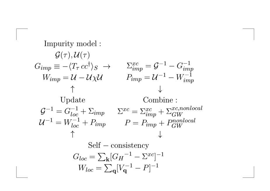
Figure 1: Schematic representation of the inner (DMFT) self-consistency cycle of the GW+DMFT scheme, consisting of the construction of the impurity model effective action (3) from the Weiss field ${\cal G}$ and the impurity Coulomb interaction ${\cal U}$, the solution of the impurity model leading to an estimate for the impurity self-energy $\Sigma_{imp}$ and the polarization $P_{imp}$ and the self-consistency condition where local quantities of the solid are calculated and then used to update the impurity model. Full self-consistency of the whole scheme requires an additional outer cycle updating the GW Hartree Potential corresponding to the obtained electronic density (cf text).

This cycle (which is summarized in Fig.1) is iterated until self-consistency for ${\cal G}$ and ${\cal U}$ is obtained (as well as on $G$, $W$, $\Sigma^{xc}$ and $P$). Eventually, self-consistency over the local electronic density can also be implemented, (in a similar way as in LDA+DMFT [29, 30]) by recalculating $\rho(\vec{r})$ from the Green’s function at the end of the convergence cycle above, and constructing an updated Hartree potential. This new density is used as an input of a new GW calculation, and convergence over this external loop must be reached.

We stress that in this scheme the Hubbard interaction ${\cal U}$ is no longer an external parameter but is determined self-consistently. The appearance of the two functions ${\cal U}$ and $W_{loc}$ might appear puzzling at first sight, but has a clear physical interpretation: $W_{loc}$ is the fully screened Coulomb interaction, while ${\cal U}$ is the Coulomb interaction screened by all electronic degrees of freedom that are not explicitly included in the effective action. So for example onsite screening is included in $W_{loc}$ but not in ${\cal U}$. From Eq. (48) it is seen that further screening of ${\cal U}$ by the onsite polarization precisely leads to $W_{loc}$.

In the following we discuss some important issues for the implementation of the proposed scheme, related to the choice of the basis functions for one-particle and two-particle quantities. In practice the self-energy is expanded in some basis set $\{\phi_{L}\}$ localized in a site. The polarization function on the other hand is expanded in a set of two-particle basis functions $\{\phi_{L}\phi_{L^{\prime}}\}$ (product basis) since the polarization corresponds to a two-particle propagator. For example, when using the linear muffin-tin orbital (LMTO) band-structure method, the product basis consists of products of LMTO’s. These product functions are generally linearly dependent and a new set of optimized product basis (OPB) [12] is constructed by forming linear combinations of product functions, eliminating the linear dependencies. We denote the OPB set by $B_{\alpha}=\sum_{LL^{\prime}}\phi_{L}\phi_{L^{\prime}}c_{LL^{\prime}}^{\alpha}$. To summarize, one-particle quantities like $G$ and $\Sigma$ are expanded in $\{\phi_{L}\}$ whereas two-particle quantities such as $P$ and $W$ are expanded in the OPB set $\{B_{\alpha}\}$. It is important to note that the number of $\{B_{\alpha}\}$ is generally smaller than the number of $\{\phi_{L}\phi_{L^{\prime}}\}$ so that quantities expressed in $\{B_{\alpha}\}$ can be expressed in $\{\phi_{L}\phi_{L^{\prime}}\}$, but not vice versa. E.g. matrix elements in products of LMTOs can be obtained from those in the $\{B_{\alpha}\}$ basis via the transformation

$$W_{L_{1}L_{2}L_{3}L_{4}}^{{\bf R}{\bf R}^{\prime}}\equiv\langle\phi_{L_{1}}^{{\bf R}}\phi_{L_{2}}^{{\bf R}}|W|\phi_{L_{3}}^{{\bf R}^{\prime}}\phi_{L_{4}}^{{\bf R}^{\prime}}\rangle=\sum_{\alpha\beta}O_{L_{1}L_{2}}^{\alpha}W_{\alpha\beta}^{{\bf R}{\bf R}^{\prime}}O_{L_{3}L_{4}}^{\beta*}$$ (49)

with the overlap matrix $O_{L_{1}L_{2}}^{\alpha}\equiv\langle\phi_{L_{1}}\phi_{L_{2}}|B^{\alpha}\rangle$, but the knowledge of the matrix elements $W_{L_{1}L_{2}L_{3}L_{4}}$ alone does not allow to go back to the $W_{\alpha\beta}$.

4 Challenges and open questions

Global self-consistency

As has been pointed out, the above GW+DMFT scheme involves self-consistency requirements at two levels: for a given density, that is Hartree potential, the dynamical mean field loop detailed in section 1 must be iterated until ${\cal G}$ and ${\cal U}$ are self-consistently determined. This results in a solution for $G$, $W$, $\Sigma^{xc}$ and $P$ corresponding to this given Hartree potential. Then, a new estimate for the density must be calculated from $G$, leading to a new estimate for the Hartree potential, which is reinserted into (45). This external loop is iterated until self-consistency over the local electronic density is reached.

The external loop is analogous to the one performed when GW calculations are done self-consistently. From calculations on the homogeneous electron gas [31] it is known, that self-consistency at this level worsens the description of spectra (and in particular washes out satellite structures) when vertex corrections are neglected. Since the combined GW+DMFT scheme, however, includes the local vertex to all orders and only neglects non-local vertex corrections we expect the situation to be more favorable in this case. Test calculations to validate this hypothesis are an important subject for future studies. First steps in this direction have been undertaken in [32].

The notion of locality : the choice of the basis set

The construction of the GW+DMFT functional $\Psi_{GW}$ crucially relies on the notion of local and nonlocal contributions. In a solid these notions can only be defined by introducing a basis set of localized functions centered on the atomic positions. Local components are then defined to be those functions the arguments of which refer to the same atomic lattice site. We stress that in this way the concept of locality is not a pointwise ($\delta$-like) one. It merely means that local quantities have an expansion (15) within their atomic sphere the form of which is determined by the basis functions used. This feature is shared between LDA+DMFT and the GW+DMFT scheme, and approaches that could directly work in the continuum are so far not in sight. If however, the basis set dependence induced by this concept is of practical importance remains to be tested.

Within LDA+DMFT the choice of the basis functions enters at two stages : First, the definition of the onsite U and the quality of the approximation consisting in the neglect of offsite interactions depends on the degree of localization of the basis functions. Second, the DMFT approximation promoting a local quantity to the full self-energy of the solid is the better justified the more localized the chosen basis functions are. However, in the spirit of obtaining an accurate low-energy description one might – depending on the material under consideration – in some cases be led to work in a Wannier function basis incorporating weak hybridisation effects of more extended states with the localized ones. This then leads to slightly more extended basis functions, and one has to compromise between maximally localized orbitals and an efficient description of low-energy bands.

In GW+DMFT, some non-local corrections to the self-energy are included, so that the DMFT approximation should be less severe. More importantly, this scheme could (via the ${\cal U}$ self-consistency requirement) automatically adapt to more or less localized basis functions by choosing itself the appropriate ${\cal U}$. Therefore, the basis set dependence is likely to be much weaker in GW+DMFT than in LDA+DMFT.

Separation of correlated and uncorrelated orbitals

As mentioned in section 1 the construction of the LDA+DMFT Hamiltonian requires an a priori choice of which orbitals are treated as correlated or uncorrelated orbitals. Since in GW+DMFT the Hubbard interactions are determined self-consistently it might be perceivable not to perform such a separation at the outset, but to rely on the self-consistency cycle to find small values for the interaction between itinerant (e.g. s or p) orbitals. Even if this issue would probably not play a role for practical calculations, it would be satisfactory from a conceptual point of view to be able to treat all orbitals on an equal footing. It is therefore also an important question for future studies.

Dynamical impurity models

Dynamical impurity models are hard to solve, since standard techniques used for the solution of static impurity models within usual DMFT, such as the Hirsch-Fye QMC algorithm or approximate techniques such as the iterative perturbation theory are not applicable. First attempts have been made in [10] and [40] using different auxiliary field QMC schemes and in [39] using an approximate “slave-rotor” scheme. These techniques, however, have so far only been applied in the context of model systems, and their implementation in a multi-band realistic calculation is at present still a challenging project. In the following section we therefore present a simplified static implementation of the GW+DMFT scheme.

5 Static implementation

Here, we demonstrate the feasibility and potential of the approach within a simplified implementation, which we apply to the electronic structure of Nickel. The main simplifications made are: (i) The DMFT local treatment is applied only to the $d$-orbitals, (ii) the GW calculation is done only once, in the form [12]: $\Sigma^{xc}_{GW}=G_{LDA}\cdot W[G_{LDA}]$, from which the non-local part of the self-energy is obtained, (iii) we replace the dynamical impurity problem by its static limit, solving the impurity model (3) for a frequency-independent ${\cal U}={\cal U}(\omega=0)$. Instead of the Hartree Hamiltonian we start from a one-electron Hamiltonian in the form: $H_{LDA}-V_{xc,\sigma}^{nonlocal}-\frac{1}{2}\mbox{\bf Tr}\Sigma_{\sigma}^{imp}(0)$. The non-local part of this Hamiltonian coincides with that of the Hartree Hamiltonian while its local part is derived from LDA, with a double-counting correction of the form proposed in [33] in the DMFT context. With this choice the self-consistency condition (45) reads:

$$G_{loc}^{\sigma}(i\omega_{n}) = \sum_{\bf k}[{G_{H}}^{-1}({\bf k},i\omega_{n})-(\Sigma^{xc}_{GW})_{non-loc}$$

$$- (\Sigma_{imp,\sigma}-\frac{1}{2}\mbox{\bf Tr}_{\sigma}\Sigma_{imp,\sigma}(0)+V_{xc}^{loc})\,]^{-1}$$

We have performed finite temperature GW and LDA+DMFT calculations (within the LMTO-ASA[21] with 29 ${\bf k}$-points in the irreducible Brillouin zone) for ferromagnetic nickel (lattice constant 6.654 a.u.), using 4s4p3d4f states, at the Matsubara frequencies $i\omega_{n}$ corresponding to $T=630K$, just below the Curie temperature. The resulting self-energies are inserted into Eq. (5), which is then used to calculate a new Weiss field according to (47). The Green’s function $G^{\sigma}_{loc}(\tau)$ is recalculated from the impurity effective action by QMC and analytically continued using the Maximum Entropy algorithm. The resulting spectral function is plotted in Fig.(2). Comparison with the LDA+DMFT results in [33] shows that the good description of the satellite structure, exchange splitting and band narrowing is indeed retained within the (simplified) GW+DMFT scheme.

Figure 2: Partial density of states of d-orbitals of nickel (solid [dashed] lines give the majority [minority] spin contribution) as obtained from the combination of GW and DMFT (see text). For comparison with LDA and LDA+DMFT results see [33], for experimental spectra see [34].

We have also calculated the quasiparticle band structure, from the poles of (5), after linearization of $\Sigma({\bf k},i\omega_{n})$ around the Fermi level . Fig. (3) shows a comparison of GW+DMFT with the LDA and experimental band structure. It is seen that GW+DMFT correctly yields the bandwidth reduction compared to the (too large) LDA value and renormalizes the bands in a (${\bf k}$-dependent) manner.

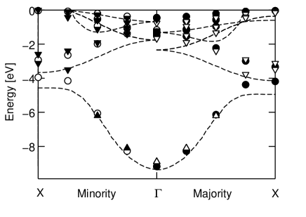
Figure 3: Band structure of Ni (minority and majority spin) as obtained from the linearization procedure of the GW+DMFT self-energy described in the text (dots) in comparison to the LDA band structure (dashed lines) and the experimental data of [35] (triangles down) and [34] (triangles up).

We now discuss further the simplifications made in our implementation. Because of the static approximation (iii), we could not implement self-consistency on $W_{loc}$ (Eq. (46)). We chose the value of ${\cal U}(\omega=0)$ ($\simeq 3.2eV$) by calculating the correlation function $\chi$ and ensuring that Eq. (43) is fulfilled at $\omega=0$, given the GW value for $W_{loc}(\omega=0)$ ($\simeq 2.2eV$ for Nickel [38]). This procedure emphasizes the low-frequency, screened value, of the effective interaction. Obviously, the resulting impurity self-energy $\Sigma_{imp}$ is then much smaller than the local component of the GW self-energy (or than $V_{xc}^{loc}$), especially at high frequencies. It is thus essential to choose the second term in (3) to be the onsite component of the GW self-energy rather than the r.h.s of Eq. (39). For the same reason, we included $V_{xc}^{loc}$ in Eq.(5) (or, said differently, we implemented a mixed scheme which starts from the LDA Hamiltonian for the local part, and thus still involves a double-counting correction). We expect that these limitations can be overcome in a self-consistent implementation with a frequency-dependent ${\cal U}(\omega)$ (hence fulfilling Eq. (39)). In practice, it might be sufficient to replace the local part of the GW self-energy by $\Sigma_{imp}$ for correlated orbitals only. Alternatively, a downfolding procedure could be used.

6 Perspectives

In conclusion, we have reviewed a recent proposal of an ab initio dynamical mean field approach for calculating the electronic structure of strongly correlated materials, which combines GW and DMFT. The scheme aims at avoiding the conceptual problems inherent to “LDA+DMFT” methods, such as double counting corrections and the use of Hubbard parameters assigned to correlated orbitals. A full practical implementation of the GW$+$DMFT scheme is a major goal for future research, which requires further work on impurity models with frequency-dependent interaction parameters [41, 42, 10] as well as studies of various possible self-consistency schemes.

7 Acknowledgments

This work was supported in part by NAREGI Nanoscience Project, Ministry of Education, Culture, Sports, Science and Technology, Japan and by a grant of supercomputing time at IDRIS Orsay, France (project number 031393).

1

References

- [1] V. I. Anisimov, J. Zaanen, and O. K. Andersen, Phys. Rev. B 44, 943 (1991)
- [2] V. I. Anisimov, I. V. Solovyev, M. A. Korotin, M. T. Czyzyk, and G. A. Sawatzky, Phys. Rev. B 48, 16929 (1993)
- [3] A. I. Lichtenstein, J. Zaanen, and V. I. Anisimov, Phys. Rev. B 52, R5467 (1995)
- [4] For a review, see V. I. Anisimov, F. Aryasetiawan, and A. I. Lichtenstein, J. Phys.: Condens. Matter 9, 767 (1997)
- [5] V. I. Anisimov et al., J. Phys.: Condens. Matter 9, 7359 (1997)
- [6] A. I. Lichtenstein and M. I. Katsnelson, Phys. Rev. B 57, 6884 (1998).
- [7] For reviews, see Strong Coulomb correlations in electronic structure calculations, edited by V. I. Anisimov, Advances in Condensed Material Science (Gordon and Breach, New York, 2001)
- [8] For related ideas, see : G. Kotliar and S. Savrasov in New Theoretical Approaches to Strongly Correlated Systems, Ed. by A. M. Tsvelik (2001) Kluwer Acad. Publ. (and the updated version: cond-mat/0208241)
- [9] S. Biermann, F. Aryasetiawan, and A. Georges, Phys. Rev. Lett. 90, 086402 (2003)
- [10] P. Sun and G. Kotliar, Phys. Rev. B 66, 085120 (2002)
- [11] L. Hedin, Phys. Rev. 139, A796 (1965); L. Hedin and S. Lundqvist, Solid State Physics vol. 23, eds. H. Ehrenreich, F. Seitz, and D. Turnbull (Academic, New York, 1969)
- [12] F. Aryasetiawan and O. Gunnarsson, Rep. Prog. Phys. 61, 237 (1998)
- [13] W. G. Aulbur, L. Jönsson, and J. W. Wilkins, Solid State Physics 54, 1 (2000)
- [14] G. Onida, L. Reining, A. Rubio, Rev. Mod. Phys. 74, 601 (2002).
- [15] W. Ku, A. G. Eguiluz, and E. W. Plummer, Phys. Rev. Lett. 85, 2410 (2000); H. Yasuhara, S. Yoshinaga, and M. Higuchi, ibid. 85, 2411 (2000)
- [16] F. Aryasetiawan, Phys. Rev. B 46, 13051 (1992)
- [17] F. Aryasetiawan and O. Gunnarsson, Phys. Rev. Lett. 74, 3221 (1995)
- [18] S. V. Faleev, M. van Schilfgaarde, and T. Kotani, unpublished
- [19] L. Hedin, Int. J. Quantum Chem. 54, 445 (1995)
- [20] For reviews, see A. Georges, G. Kotliar, W. Krauth, and M. J. Rozenberg, Rev. Mod. Phys. 68, 13 (1996); T. Pruschke et al, Adv. Phys. 44, 187 (1995)
- [21] O. K. Andersen, Phys. Rev. B 12, 3060 (1975); O. K. Andersen, T. Saha-Dasgupta, S. Erzhov, Bul. Mater. Sci. 26, 19 (2003)
- [22] Q. Si and J. L. Smith, Phys. Rev. Lett. 77, 3391 (1996)
- [23] G. Kotliar and H. Kajueter (unpublished)
- [24] H. Kajueter, Ph.D. thesis, Rutgers University, 1996
- [25] A. M. Sengupta and A. Georges, Phys. Rev. B 52, 10295 (1995)
- [26] F. Aryasetiawan, M. Imada, A. Georges, G. Kotliar, S. Biermann, and A. I. Lichtenstein, submitted to Phys. Rev. B.
- [27] C.-O. Almbladh, U. von Barth and R. van Leeuwen, Int. J. Mod. Phys. B 13, 535 (1999)
- [28] R. Chitra and G. Kotliar, Phys. Rev. B 63, 115110 (2001)
- [29] S. Savrasov and G. Kotliar, cond-mat/0106308
- [30] S. Savrasov, G. Kotliar and E. Abrahams, Nature (London) 410, 793 (2000)
- [31] B. Holm and U. von Barth, Phys. Rev. B 57, 2108 (1998)
- [32] P. Sun and G. Kotliar, cond-mat/0312303
- [33] A. I. Lichtenstein, M. I. Katsnelson and G. Kotliar, Phys. Rev. Lett. 87, 067205 (2001)
- [34] H. Mårtensson and P. O. Nilsson, Phys. Rev. B 30, 3047 (1984)
- [35] J. Bünemann et al, Europhys. Lett. 61, 667 (2003)
- [36] Y. Motome and G. Kotliar, Phys. Rev. B 62, 12800 (2000)
- [37] J. K. Freericks, M. Jarrell and D. J. Scalapino, Phys. Rev. B 48, 6302 (1993)
- [38] M. Springer and F. Aryasetiawan, Phys. Rev. B 57, 4364 (1998)
- [39] S. Florens, PhD thesis, Paris 2003 ; S. Florens, A. Georges, L. Demedici, unpublished.
- [40] A. Rubtsov, unpublished.
- [41] Y. Motome, G. Kotliar, Phys. Rev. B 62, 12800 (2000).
- [42] J. K. Freericks, M. Jarrell, D. J. Scalapino, Phys. Rev. B 48, 6302 (1993).