Ferrimagnetic mixed-spin ladders in weak and strong coupling limits

Abstract

We study two similar spin ladder systems with the ferromagnetic leg coupling. First model includes two sorts of spins, $s=1/2$ and $s=1$, and the second model comprises only $s=1/2$ legs coupled by a ”triangular” rung exchange. We show that the antiferromagnetic (AF) rung coupling destroys the long-range order and eventually makes the systems equivalent to the AF $s=1/2$ Heisenberg chain. We study the crossover from the weak to strong coupling regime by different methods, particularly by comparing the results of the spin-wave theory and the bosonization approach. We argue that the crossover regime is characterized by the gapless spectrum and non-universal critical exponents are different from those in XXZ model.

I introduction

The strongly correlated systems in one spatial dimension (1D) attracted an enormous theoretical and experimental interest last decade. The 1D fermionic and spin systems were recognized long ago as the useful theoretical models, where the interaction effects are very important and at the same time are subject to rigorous analysis. GoNeTs ; SchulzCuPi The experimental discovery of the systems of predominantly 1D character inspired the renewed interest to this class of problems. Among the experimental realizations of the 1D systems one can mention the Bechgaards salts, carbon nanotubes, copper oxides spin ladders and purely organic spin chain compounds. GoNeTs

While the physics of purely one-dimensional objects, or chains, is well understood, GoNeTs ; SchulzCuPi the spin ladders are still under intense investigation. Even the isolated spin chains reveal a variety of unusual phenomena, including the Haldane gap, spin-Peierls transition, magnetization plateaus. The ladders, consisting of a few coupled spin chains are generally much richer in their behavior, and pose additional theoretical problems.

The interest to the problem of ladders may be traced back to the earlier attempts to construct the continous representation of spin $S=1$ variable in 1D out of $s=1/2$ quantities. Schulz86 The methods elaborated in these studies are now widely used in the analysis of the ladder systems.

The basic model for the spin chain, the antiferromagnetic (AF) Heisenberg $s=1/2$ chain, is thoroughly studied by various methods. GoNeTs This may be one of the reasons, why a majority of the theoretical papers discussing the spin ladders are now confined to the treatment of quantum spin $s=1/2$ with antiferromagnetic interaction along the legs. Spin ladders with different spins or with a ferromagnetic leg exchange attracted much less attention.

The spin chains and ladders consisting of different spins organic and with the AF leg exchange were considered recently in Ivanov01 ; Brehmer97 ; Wu99 ; TruGa01 ; Sakai02 . Particularly, the ferrimagnetic chains with alternating spin-1/2 and spin-1 were discussed there. It was shown that, contrary to the case of equal spins, the uncompensated spin value in a unit cell leads to the gap in the spectrum and the appearance of the long range magnetic order. Tian97

The spin-1/2 ladder with ferromagnetic exchange along the legs was studied in Roji96 ; Vekua03 . A rather rich phase diagram was demonstrated, depending on the details of the magnetic anisotropies for the leg and rung couplings.

In the present paper we study the mixed spin ($S=1$, $s=1/2$) spin ladder with the ferromagnetic exchange along the legs and antiferromagnetic interaction on the rungs.In the absence of the rung coupling, the individual chains show the ferromagnetic long-range order (LRO), and the ground state is classical. The spectrum and the ground state energy is well described in terms of the linear spin-wave theory. Ivanov01 We show that the inclusion of the antiferromagnetic rung coupling drives the system into the quantum regime, understood in terms of the AF Heisenberg spin-1/2 chain. In this regime the magnetic LRO is absent, and the spatial correlations show the power-law decay. Note that the uncompensated spin in a unit cell leads to the absence of the gap in low-lying excitation spectra.

This primary observation is interesting on its own, because two limiting cases of the model allow the asymptotically exact solutions with gapless spectra. Hence our further motivation to study the crossover region starting from both limiting points.

We discuss the regimes of weak and strong rung coupling for different types of the leg exchange anisotropy. The consideration is somewhat complicated by the absence of the established routines for our case. The bosonization, an extremely useful tool in dealing with AF s=1/2 systems, does not fully work here on two reasons. First is the existence of two sorts of spins in a unit cell, and another is the ferromagnetic leg exchange.

Hence we supplement our study by the consideration of a similar model, written entirely for $s=1/2$ but with the modified rung couplings. Using these models and comparing different approaches, the spin-wave theory and bosonization, we arrive at the unified description of the ferrimagnetic spin ladders. Particuarly, we discuss the spectrum and the correlations and observe the crossover from the weak to strong coupling regime. An attention is paid to a subtler point in the bosonization procedure, a seemingly unstable Gaussian effective action near the ferromagnetic point.

The rest of the paper is organized as follows. We discuss the mixed spin model in strong and weak rung coupling regime in Sec. II. The spin $s=1/2$ ladder with ”triangular” rung exchange is introduced and analyzed in Sec. III. The existence of different order parameters in a system is discussed in Sec. IV. The discussion and conclusions are in Sec. V

II mixed spin ladder

We investigate the properties of a ladder system, consisting of two sorts of spins, $s=1/2$ and $S=1$, arranged in a checkerboard manner. The unit cell comprises four spins and the Hamiltonian is

$${\cal H} = -\sum_{i}J_{\|}^{\alpha}\left({s}_{1,2i}^{\alpha}{S}_{1,2i\pm 1}^{\alpha}+{s}_{2,2i\pm 1}^{\alpha}{S}_{2,2i}^{\alpha}\right)$$ (1)

$$+J_{\perp}\sum_{i}\left({\bf s}_{1,2i}{\bf S}_{2,2i}+{\bf S}_{1,2i+1}{\bf s}_{2,2i+1}\right)$$

with the first subscript (e.g.  1 in ${\bf s}_{1,2i}$) labeling the leg, and the second one denoting the site on it (odd or even). Below we mostly consider the case of the AF rung coupling, $J_{\perp}>0$. The overall ferromagnetic exchange along the chains allows the uniaxial anisotropy, $J_{\|}^{x}=J_{\|}^{y}=J>0$, $J_{\|}^{z}=J+D>0$, $|D|\ll J$. In what follows, we consider also a useful generalization to higher spins, $s\gg 1$ with the difference $S-s=1/2$ kept fixed. The whole consideration is done for zero temperature.

First let us briefly describe two simple limiting cases. At $D=0+$ and $J_{\perp}=0$, we have two ferromagnetic chains, which possess the long-range magnetic order. The spectrum is quadratic at small wave vectors, $\omega\sim Jq^{2}$. We put the lattice spacing $a$ to unity everywhere except the Sec. III.4.

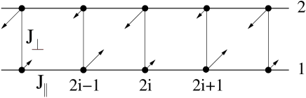
Figure 1: A ladder of spins $S=1$, $s=1/2$

In the opposite limiting case, $J_{\perp}\gg J$, the ground state of two spins on the rung, say, ${\bf s}_{1,2i}$ and ${\bf S}_{2,2i}$ is doublet, described by a spin $s=1/2$ variable ${\bf\sigma}_{2i}$. We show below, that the effective interaction between these ${\bf\sigma}_{i}$ is antiferromagnetic for the above choice $J>0$ and hence the situation is mapped onto a well-known problem of $s=1/2$ Heisenberg antiferromagnet. One does not expect the long-range order at $D=0$ and the spectrum is linear $\varepsilon_{k}\sim Jk$. The correlation functions for this case are described below.

The intermediate situation, $J\sim J_{\perp}$, $D\neq 0$, is harder to analyze and we present several ways to discuss it below.

II.1 Strong rung coupling

Consider first the case of strong perpendicular coupling, $J_{\perp}\gg J$. Taking first $J=D=0$, one sees that each pair of spins $s,S$ is characterized by a total spin ${\bf j}={\bf s}+{\bf S}$ and by the rung energy $E_{j}=J_{\perp}{\bf s}{\bf S}=\frac{1}{2}J_{\perp}(j(j+1)-s(s+1)-S(S+1))$. The lowest state here is doublet, $j=1/2$, the first excited state is quadruplet $j=3/2$, with $E_{3/2}-E_{1/2}=3J_{\perp}/2$. The wave function of a multiplet is

$$|j,m\rangle=\sum_{m_{1},m_{2}}C^{jm}_{sm_{1}Sm_{2}}|sm_{1}\rangle|Sm_{2}\rangle$$ (2)

with Clebsch-Gordan coefficients $C^{jm}_{sm_{1}Sm_{2}}$. The interaction along the chain is considered now as a perturbation. The formula (2) and consideration below are applicable for larger spins as well. In this more general case of $s=S-1/2\geq 1/2$, the operators $s^{\alpha}$, $S^{\alpha}$ act within the lowest doublet and connect the doublet with the quadruplet, but the direct transitions to the higher states, $j=1/2\to j\geq 5/2$, are absent. One can check that the corresponding matrix elements are given by

$$\langle j=1/2,m|s^{\alpha}|j=1/2,m^{\prime}\rangle = -\frac{s}{3}\sigma^{\alpha}_{mm^{\prime}},$$

$$\langle j=1/2,m|S^{\alpha}|j=1/2,m^{\prime}\rangle = \frac{S+1}{3}\sigma^{\alpha}_{mm^{\prime}},$$ (3)

with $\sigma^{\alpha}_{mm^{\prime}}$ the Pauli matrices. For $s=1/2$ this reads

$$s^{\alpha}\leftrightarrow-\frac{1}{6}\sigma^{\alpha},\quad S^{\alpha}\leftrightarrow\frac{2}{3}\sigma^{\alpha}.$$ (4)

It shows that if we consider only the projection of the spin operators onto the lowest doublet, then the above Hamiltonian corresponds to the AF Heisenberg spin-$1/2$ model of the form :

$${\cal H}_{eff}=\sum_{i}J_{eff}^{\alpha}\sigma_{i}^{\alpha}\sigma_{i+1}^{\alpha},$$ (5)

where

$$J_{eff}^{\alpha}(J_{\perp}\to\infty)=2J_{\|}^{\alpha}s(S+1)/9.$$ (6)

Below we will refer to this estimate of $J_{eff}^{\alpha}$ as $J_{eff}^{\alpha}(\infty)$. For $s=1/2$ we have $J_{eff}^{\alpha}(\infty)=2J_{\|}^{\alpha}/9$.

Let us next consider the role of the higher states on a rung. We do not list here the matrix elements of the spin operators $S^{\alpha}$, $s^{\alpha}$ for the transitions $j=1/2\to j=3/2$. We only note that they are proportional to $\sqrt{s(S+1)}$ and are the same for $S^{\alpha}$ and $s^{\alpha}$, except for the sign. The second-order correction in $J_{\|}$ between the adjacent rungs, labeled by 1 and 2 below, can be written as

$$J_{\|}^{\alpha}J_{\|}^{\beta}\frac{4\langle\frac{1}{2}|s_{1}^{\alpha}|\frac{3}{2}\rangle\langle\frac{3}{2}|s_{1}^{\beta}|\frac{1}{2}\rangle\langle\frac{1}{2}|S_{2}^{\alpha}|\frac{3}{2}\rangle\langle\frac{3}{2}|S_{2}^{\beta}|\frac{1}{2}\rangle}{2E_{1/2}-2E_{3/2}},$$ (7)

with factor 4 coming from the above property of coincidence of the matrix elements. Noting that

$$\langle\frac{1}{2},m|s_{1}^{\alpha}|\frac{3}{2}\rangle\langle\frac{3}{2}|s_{1}^{\beta}|\frac{1}{2},m^{\prime}\rangle$$

$$=\frac{s(S+1)}{9}(2\delta_{\alpha\beta}\delta_{mm^{\prime}}-i\epsilon_{\alpha\beta\gamma}\sigma^{\gamma}_{mm^{\prime}}),$$ (8)

we find that the second order in $J_{\|}$ results in (5) with the renormalized value of effective interaction :

$$J_{eff}^{\alpha}(J_{\perp})=J_{eff}^{\alpha}(\infty)+\epsilon^{2}_{\alpha\beta\gamma}\frac{J_{eff}^{\beta}(\infty)J_{eff}^{\gamma}(\infty)}{9J_{\perp}}.$$ (9)

with $J_{eff}^{\alpha}$ from (6). For the above parameters $J_{\|}^{\alpha}$ and $s=1/2$ one has

$$J_{eff}^{x} = J_{eff}^{y}=\frac{2}{9}J+\frac{8J(J+D)}{729J_{\perp}},$$ (10)

$$J_{eff}^{z} = \frac{2}{9}(J+D)+\frac{8J^{2}}{729J_{\perp}},$$ (11)

which particularly means that the relative value of anisotropy decreases with decreasing $J_{\perp}$. The perturbation theory is expected to break down when the correction in $J_{\perp}^{-1}$ is comparable to the first term in (9), which happens roughly at $J_{\perp}\sim J_{\|}^{\alpha}s^{2}$. Note that this criterion also corresponds to the point where the bandwidth induced by $J_{eff}$ becomes comparable to the separation $\sim J_{\perp}$ between the quadrupet and doublet. At larger $J_{\perp}$ the low-energy dynamics is described by the AF spin-one-half XXZ model (5) which is exactly solvable.

In the isotropic case, $D=0$, the spectrum is linear, $\omega=\frac{\pi}{8}J_{eff}|q|$ and the correlations are of the form

$$\langle\sigma^{\alpha}_{i}\sigma^{\alpha}_{i+n}\rangle\sim|n|^{-2}+(-1)^{n}|n|^{-1},$$

with the omitted minor logarithmic corrections. Aff-log

Taking into account the matrix elements (3) we find that the leading asymptotes in the isotropic, $s=1/2,S=1$ case are :

$$\langle s^{\alpha}_{1,i}s^{\alpha}_{1,i+2n}\rangle \sim |2n|^{-1}$$

$$\langle s^{\alpha}_{1,i}S^{\alpha}_{1,i+2n+1}\rangle \sim 4|2n+1|^{-1}$$ (12)

$$\langle S^{\alpha}_{1,i}S^{\alpha}_{1,i+2n}\rangle \sim 16|2n|^{-1}$$

Thus the long-range ferromagnetic order is absent, but the correlations are ferromagnetic and slowly decaying. In addition, there is a subleading sign-reversal asymptote and modulation depending on the spin value ($s=1/2,1$). The correlations between the spins in different chains are slowly decaying antiferromagnetic ones, e.g. $\langle s^{\alpha}_{1,i}s^{\alpha}_{2,i+2n+1}\rangle\sim-|2n+1|^{-1}$. The above form of the correlations is obviously unchanged as long as $J_{\perp}\lesssim J$.

II.2 Weak rung coupling, spin-wave analysis

Let us consider next the opposite limiting case, when the leg exchange dominates and $J_{\perp}$ can be considered as perturbation. First we explore the spin-wave formalism for the easy-axis anisotropy, $D>0$. It was shown recently Ivanov01 that in case of ferrimagnetic system in 1D the spin-wave description gives very good estimate for the ground state energy and on-site magnetization. Performing the standard Dyson-Maleyev expansion,

$$S^{z}_{1} = -S+a^{\dagger}a,\quad s^{z}_{1}=-s+b^{\dagger}b$$

$$S^{+}_{1} = \sqrt{2S}a^{\dagger}(1-a^{\dagger}a/(2S)),$$

$$s^{+}_{1} = \sqrt{2s}b^{\dagger}(1-b^{\dagger}b/(2s))$$

$$S^{-}_{1} = \sqrt{2S}a,\quad s^{-}_{1}=\sqrt{2s}b$$

$$S^{z}_{2} = S-c^{\dagger}c,\quad s^{z}_{2}=s-d^{\dagger}d$$

$$S^{+}_{2} = \sqrt{2S}(1-c^{\dagger}c/(2S))c,$$

$$s^{+}_{2} = \sqrt{2s}(1-d^{\dagger}d/(2s))d$$

$$S^{-}_{2} = \sqrt{2S}c^{\dagger},\quad s^{-}_{2}=\sqrt{2s}d^{\dagger}$$ (13)

we write for the magnon Green function in the linear spin-wave theory (LSWT) approximation

$$\Phi^{\dagger} = (a_{k}^{\dagger},b_{k}^{\dagger},c_{-k},d_{-k})$$

$$G_{ij}(k,t) = -i\theta(t)\langle[\Phi_{i}(k,t),\Phi^{\dagger}_{j}(k,0)]\rangle$$ (14)

$$G(k,\omega)^{-1} = -\begin{pmatrix}s(2J_{\|}^{z}+J_{\perp})-\omega&\sqrt{sS}J\gamma_{k}&0&\sqrt{sS}J_{\perp}\\ \sqrt{sS}J\gamma_{k}&S(2J_{\|}^{z}+J_{\perp})-\omega&\sqrt{sS}J_{\perp}&0\\ 0&\sqrt{sS}J_{\perp}&s(2J_{\|}^{z}+J_{\perp})+\omega&\sqrt{sS}J\gamma_{k}\\ \sqrt{sS}J_{\perp}&0&\sqrt{sS}J\gamma_{k}&S(2J_{\|}^{z}+J_{\perp})+\omega\end{pmatrix}$$ (15)

Here $\gamma_{k}=2\cos k$. The spectrum consists of doubly degenerate acoustic and optical modes. The optical mode has the energy $\sim\sqrt{sS}J$ for all wave vectors and the acoustic branch at small $k$ is

$$\varepsilon_{k}\simeq\frac{2sS}{s+S}\sqrt{(2D+Jk^{2})(2D+Jk^{2}+2J_{\perp})}$$ (16)

so instead of the quadratic spectrum of purely FM case, we have an approximately linear spectrum at small energies $\varepsilon_{k}\lesssim sJ_{\perp}$. The contribution of the zero-point fluctuations into the average on-site magnetization can be estimated for $D\ll J_{\perp}\ll J$ as follows

$$s-\langle s_{1i}\rangle\sim\sqrt{J_{\perp}/J}\ln(\sqrt{J_{\perp}/D}).$$ (17)

It means that the spin-wave approximation fails when the latter quantity is of order of $s$. It happens roughly at $J_{\perp}\gtrsim s^{2}J(\ln s^{2}J/D)^{-2}$, which corresponds to the crossover point $\gamma^{\ast}$ in Roji96 . Apart from the logarithmic factor, this estimate agrees with the above value $J_{\perp}\sim s^{2}J_{\|}$, obtained in the large $J_{\perp}$ limit. For lower $J_{\perp}$ the system shows the long-range order.

It might be instructive to consider the FM rung coupling $J_{\perp}<0$. In this case all the branches of the spectrum are gapful, the lowest modes are

$$\varepsilon_{1,k} \simeq \frac{2sS}{s+S}(2D+Jk^{2}),$$

$$\varepsilon_{2,k} \simeq \frac{2sS}{s+S}(2D+2|J_{\perp}|+Jk^{2}),$$ (18)

Note that at the isotropic point $D=0$, the long-range FM order and hence the applicability of the LSWT is lost for any $J_{\perp}>0$. The spectrum (16) in this case is gapless and linear with the spin-wave velocity $\sim s\sqrt{JJ_{\perp}}$, the limit of $s\simeq S\gg 1$ is assumed. We know that increasing $J_{\perp}$ we should eventually recover the effective model (5), characterized by spinon velocity $\sim s^{2}J$. These two velocities match again at $J_{\perp}\sim s^{2}J$.

Concluding this section, we also present the LSWT results for the lowest branches of dispersion for the case of easy-plane anisotropy, $D<0$. For the AF sign of the exchange $J_{\perp}$ one has

$$\varepsilon_{1,k} \simeq \frac{2sS}{s+S}\sqrt{Jk^{2}(2|D|+Jk^{2}+2J_{\perp})},$$

$$\varepsilon_{2,k} \simeq \frac{2sS}{s+S}\sqrt{(2|D|+Jk^{2})(2J_{\perp}+Jk^{2})},$$ (19)

while for the FM exchange $J_{\perp}<0$ we obtain

$$\varepsilon_{1,k} \simeq \frac{2sS}{s+S}\sqrt{Jk^{2}(2|D|+Jk^{2})},$$ (20)

$$\varepsilon_{2,k} \simeq \frac{2sS}{s+S}\sqrt{(2|J_{\perp}|+Jk^{2})(2|D|+2|J_{\perp}|+Jk^{2})},$$

In this case LSWT is formally inapplicable, but the above formulas might be useful for a comparison with further results.

Summarizing, we observe that while the LSWT cannot treat the correlations correctly and formally is inapplicable in the absence of the LRO, it provides simple and reasonable formulas for the excitation spectra in a complicated one-dimensional ladder. We illustrate this point below by discussing the spin-1/2 ladder, where a rigorous description of the low-energy action is available.

II.3 Equations of motion

This subsection is devoted to the macroscopic equations describing the behavior of spins in two coupled chains. To make our calculations more transparent, we define new operators on a rung as superpositions of two spin operators

$$Q^{\alpha}_{2i} = S^{\alpha}_{2,2i}+s^{\alpha}_{1,2i},\quad R^{\alpha}_{2i}=S^{\alpha}_{2,2i}-s^{\alpha}_{1,2i},$$ (21)

$$Q^{\alpha}_{2i+1} = S^{\alpha}_{1,2i+1}+s^{\alpha}_{2,2i+1},\quad R^{\alpha}_{2i+1}=S^{\alpha}_{1,2i+1}-s^{\alpha}_{2,2i+1},$$

satisfying the following commutation relations:

$$[Q_{i}^{\alpha},Q_{i}^{\beta}] = i\epsilon_{\alpha\beta\gamma}Q_{i}^{\gamma},\quad[R_{i}^{\alpha},R_{i}^{\beta}]=i\epsilon_{\alpha\beta\gamma}Q_{i}^{\gamma},$$

$${}[R_{i}^{\alpha},Q_{i}^{\beta}] = i\epsilon_{\alpha\beta\gamma}R_{i}^{\gamma}.$$ (22)

with $\epsilon_{\alpha\beta\gamma}$ totally antisymmetric tensor ; the operators $Q^{\alpha}$ and $R^{\alpha}$ commute at different sites.

The commutation relations (22) define the $SU(2)\bigotimes SU(2)=SO(4)$ group with two Casimir operators given by

$${\bf Q\cdot R}=\frac{5}{4},\quad{\bf Q}^{2}+{\bf R}^{2}=\frac{11}{2}.$$ (23)

The Hamiltonian $H=H_{\parallel}+H_{\perp}$ takes the form

$$H_{\parallel} = -\frac{1}{2}\sum_{i}J_{\parallel}^{\alpha}\left(Q^{\alpha}_{i}Q^{\alpha}_{i+1}-R^{\alpha}_{i}R^{\alpha}_{i+1}\right)$$

$$H_{\perp} = \frac{J_{\perp}}{4}\sum_{i}\left({\bf Q}^{2}_{i}-{\bf R}^{2}_{i}\right)=\frac{J_{\perp}}{2}\sum_{i}{\bf Q}^{2}_{i}+cst$$ (24)

The equation of motions for operators ${\bf Q}$ and ${\bf R}$ are given by

$$\dot{Q}^{\alpha}_{j}=i[H,Q^{\alpha}_{j}],\quad\dot{R}^{\alpha}_{j}=i[H,R^{\alpha}_{j}].$$ (25)

These equations correspond to the well-known Bloch equations for precession of the magnetic moment of ferromagnets (antiferromagnets). Taking into account that the operators $Q^{\alpha}$ $(R^{\alpha})$ are different on two different sublattices corresponding to odd(even) sites, we use the properties

$$[{\bf Q}_{i}^{2},Q_{i}^{\alpha}]=[{\bf R}_{i}^{2},Q_{i}^{\alpha}]=0,$$

$$[{\bf Q}_{i}^{2},R_{i}^{\alpha}]=-[{\bf R}_{i}^{2},R_{i}^{\alpha}]=i\epsilon_{\alpha\beta\gamma}\{R_{i}^{\beta}Q_{i}^{\gamma}\}$$

and adopt a symbolic notation

$$i\epsilon_{\alpha\beta\gamma}\{R_{i}^{\beta}Q_{i}^{\gamma}\}=i\left({\bf R}_{i}\times{\bf Q}_{i}-{\bf Q}_{i}\times{\bf R}_{i}\right)^{\alpha}.$$

Then we obtain the following system of coupled Bloch equations for the isotropic $J_{\|}^{\alpha}$

$$\partial_{t}{\bf Q}_{i} = \frac{J_{\parallel}}{2}\left({\bf Q}_{i}\times{\bf Q}_{i\pm 1}-{\bf R}_{i}\times{\bf R}_{i\pm 1}\right)$$

$$\partial_{t}{\bf R}_{i} = \frac{J_{\parallel}}{2}\left({\bf Q}_{i}\times{\bf R}_{i\pm 1}-{\bf R}_{i}\times{\bf Q}_{i\pm 1}\right)+$$ (26)

$$+ \frac{J_{\perp}}{2}\left({\bf Q}_{i}\times{\bf R}_{i}-{\bf R}_{i}\times{\bf Q}_{i}\right).$$

Taking the continuum limit here, one has:

$$\partial_{t}{\bf Q} = \left(A_{\alpha\beta}{\bf Q}\times\frac{\partial^{2}{\bf Q}}{\partial x_{\alpha}\partial x_{\beta}}-B_{\alpha\beta}{\bf R}\times\frac{\partial^{2}{\bf R}}{\partial x_{\alpha}\partial x_{\beta}}\right)$$

$$\partial_{t}{\bf R} = \left(B_{\alpha\beta}{\bf Q}\times\frac{\partial^{2}{\bf R}}{\partial x_{\alpha}\partial x_{\beta}}-A_{\alpha\beta}{\bf R}\times\frac{\partial^{2}{\bf Q}}{\partial x_{\alpha}\partial x_{\beta}}\right)+$$ (27)

$$+ C\left({\bf Q}\times{\bf R}-{\bf R}\times{\bf Q}\right).$$

where for asymmetric two-leg ladder $\alpha=\beta=x$ and $A_{xx}=B_{xx}=J_{\parallel}a^{2}/2,\;\;C=J_{\perp}/2$. The lattice index $i$ is omitted. Being re-written in terms of densities of magnetic moments, equations (27)correspond to the generalized Landau-Lifshitz equations for the dynamic $SO(4)$ group. Note that the operator ${\bf Q}$ represents a total spin on the rung, and the operator ${\bf R}$ does not have a simple interpretation.

We introduce the densities of magnetic moment characterizing two sublattices

$${\bf M} = \frac{2}{{\cal N}}\sum_{l}{\bf Q}_{l},\quad{\bf N}=\frac{2}{{\cal N}}\sum_{l}(-1)^{l}{\bf Q}_{l},$$

$${\bf O} = \frac{2}{{\cal N}}\sum_{l}{\bf R}_{l},\quad{\bf T}=\frac{2}{{\cal N}}\sum_{l}(-1)^{l}{\bf R}_{l},$$ (28)

with ${\cal N}$ being total number of rungs in the ladder.

Obviously, ${\bf M}$ and ${\bf N}$ represent the uniform and staggered magnetizations along the ladder, whereas ${\bf T}$ and ${\bf O}$ can be interpreted as “staggered rung” magnetization in the uniform and staggered channels along the chain, respectively. The different ordered phases are charactererized by nontrivial values of ${\bf M,N,O,T}$ or some combinations of them whereas in disordered phase these quantities are equal to zero. For example, the ordered FM phase is characterized by ${\bf M}\neq 0$. In Neel phase ${\bf N}\neq 0$. In ferrimagnetic phase both ${\bf M}\neq 0$ and ${\bf N}\neq 0$. Therefore, the information about the order parameter is necessary for deriving the macroscopic Landau-Lifshitz equations from the microscopic Bloch equations.

We point out that the scalar product of two spins on a rung

$${\bf s}_{1}{\bf S}_{2}=\frac{1}{4}\left({\bf Q}^{2}-{\bf R}^{2}\right)$$

may also be considered as a local order parameter (see discussion in the Section III).

Eqs.  (26) are the central result of this subsection. Upon the assumption of the certain order parameter(s) they lead to macroscopic “equations of motion”. Applying a standard routine LL9 one can show that these equations are equivalent to LSWT treatment and reproduce magnon dispersion laws discussed in the previous subsection. The detailed analysis of the Bloch equations for asymmetric $SO(4)$ ladders will be presented elsewhere.

III triangular $s=1/2$ ladder

One may regard spin 1 as a ground state triplet of two spins 1/2 coupled ferromagnetically. Our model assumes that this triplet is also FM coupled to other spins 1/2 on a chain. Therefore instead of the FM chain of $n$ spins 1 and $n$ spins 1/2, one may consider $3n$ spins 1/2. The model we propose is

$${\cal H} = -\sum_{i}J_{\|}^{\alpha}\left({s}_{1,i}^{\alpha}{s}_{1,i+1}^{\alpha}+{s}_{2,i}^{\alpha}{s}_{2,i+1}^{\alpha}\right)$$ (29)

$$+J_{\perp}\sum_{i}\left[{\bf s}_{1,3i}\left({\bf s}_{2,3i}+{\bf s}_{2,3i+1}\right)\right.$$

$$\left.+\left({\bf s}_{1,3i+1}+{\bf s}_{1,3i+2}\right){\bf s}_{2,3i+2}\right]$$

with the above choice of $J_{\|}^{\alpha}$. The model (29) is not equivalent to the previous one, eq. (1). Indeed, the exact mapping of (1) to (29) would include the strong trimerized isotropic FM in-chain exchange, at those links which form the bases of the triangles in Fig. 2. In that case one would first consider the triangles and then couple them to each other, fully restoring the consideration of the previous Section. We show below that the model (29) with uniform value of the rung exchange has two advantages. First, it is equivalent to (1) at $J_{\perp}\to\infty$ and second, it is easier tractable in the opposite case $J_{\perp}\to 0$, since the exact form of the low-energy action is available for the uniform $J_{\|}^{\alpha}$.

Figure 2: A triangular ladder of spins $s=1/2$

III.1 Strong rung coupling

We consider a case when the AF exchange $J_{\perp}$ is much larger than $J_{\|}^{\alpha}$, first for the isotropic $J_{\|}^{\alpha}=J_{\|}$. In this case a main block is a triangle formed by two rungs, and the coupling of triangles is a perturbation. The Hamiltonian for the triangle is

$$H_{\triangle}=J_{\perp}({\bf s}_{1}+{\bf s}_{2}){\bf s}_{3}-J_{\|}({\bf s}_{1}{\bf s}_{2}-1/4)$$ (30)

The structure of the energy levels is as follows. The term $J_{\|}$ groups the spins on one leg, ${\bf s}_{1}$ and ${\bf s}_{2}$, into a triplet $|{\cal T}\rangle$ and a singlet $|{\cal S}\rangle$. The singlet does not couple to ${\bf s}_{3}$ and results in a total doublet denoted as $|D0\rangle$ with the energy $E_{D0}=J_{\|}$. The triplet $|{\cal T}\rangle$ of zero energy couples to ${\bf s}_{3}$ with the formation of doublet $|D1\rangle$ and quadruplet $|Q\rangle$. The corresponding energies are $E_{D1}=-J_{\perp}$ and $E_{Q}=J_{\perp}/2$. For $J_{\|}\to\infty$ the state $|D0\rangle$ is unimportant, and ${\bf s}_{1}$, ${\bf s}_{2}$ act as one spin $S=1$. At the same time, the low-energy sector of the problem is associated with the doublet $|D1\rangle$, and this doublet is the lowest state also for the situation $J_{\perp}\gg J_{\|}$. Therefore the strong coupling limit of the asymmetric ladder with two spins $s=1$, $s=1/2$ is described as well by the triangular lattice depicted in Fig.(2) in the same limit. The demand for in-triangle $J_{\|}$ to be large, in order to organize the effective spin-1, is relaxed in this limit, and one can consider the situation with the uniform value of the exchange $J_{\|}$ along the whole leg.

The presence of the anisotropy term $-Ds^{z}_{1}s^{z}_{2}$ in (29) is a negligible effect in the described picture. Indeed, this term translates into a single-ion anisotropy of the triplet state, $(S^{z})^{2}$ and the application of the formulas (3), (8) shows that it is only the higher $|Q\rangle$ state, which becomes split accordingly, $\sim D(S^{z})^{2}$.

Let us discuss the analog of Eq. (9) for the Hamiltonian (29). In the limit $J_{\perp}\to\infty$ the effective interaction is given by (5) with $\sigma^{\alpha}$ acting within $|D1\rangle$ and $J^{\alpha}_{eff}(\infty)=\frac{1}{9}J^{\alpha}_{\|}$. The analog of (4) for eq. (30) reads

$$s^{\alpha}_{1,2}\leftrightarrow\frac{1}{3}\sigma^{\alpha},\quad s^{\alpha}_{3}\leftrightarrow-\frac{1}{6}\sigma^{\alpha}.$$ (31)

The second order in $J^{\alpha}_{\|}$ corresponds to transitions to higher $|D0\rangle$ and $|Q\rangle$ states. After some calculations we find

$$J_{eff}^{\alpha}(J_{\perp}) \simeq J_{eff}^{\alpha}(\infty)$$

$$+\epsilon^{2}_{\alpha\beta\gamma}J_{eff}^{\beta}(\infty)J_{eff}^{\gamma}(\infty)\left[\frac{1}{3J_{\perp}}-\frac{3}{5J_{\perp}+2J}\right].$$

In (III.1) the second term is negative for $J_{\perp}\gtrsim J$, in contrast to (9). It means that the value of $J_{eff}$ and the relative exchange anisotropy $J_{eff}^{z}/J_{eff}^{x}-1$ increase with decreasing of $J_{\perp}$.

Thus we conclude that the strong coupling limit of the the trinagular ladder is described by the Hamiltonian (5) with $J_{eff}$ given by (III.1). Similarly to (12), the in-leg correlations are slowly decaying ferromagnetic ones, although their modulation is different due to eq. (31) instead of (4).

III.2 Weak rung coupling, LSWT analysis

For the case of ferromagnetic exchange with the easy-axis anisotropy we employ the spin-wave formalism. The situation is complicated by the existence of six spins in a unit cell. As a result, the quadratic Hamiltonian is represented as $6\times 6$ matrix. The Hamiltonian for the interaction along the leg is standard, while the rung exchange needs some care.

Consider first two quantities $A_{i}$ and $B_{i}$ referring to $i$th site on the upper and lower leg, respectively. If $A_{i}$ and $B_{i}$ are coupled by the triangular rung exchange, Fig. 2, then we have an expression

$$J_{\perp}\sum_{j}(A_{3j}+A_{3j+1})B_{3j}+A_{3j+2}(B_{3j+1}+B_{3j+2}),$$ (33)

with one term in the sum (33) describing the coupling in the unit cell, and three-site periodicity of the overall structure. Going to Fourier components we have

$$\sum_{q}A_{q}(B_{-q}g_{q}+B_{-q+\kappa}f_{q}+B_{-q-\kappa}f^{\ast}_{-q}),$$ (34)

with $\kappa=2\pi/3$ and

$$g_{q}=\frac{2}{3}J_{\perp}(1+e^{iq})\quad f_{q}=-\frac{1}{3}J_{\perp}(e^{i\kappa}+e^{iq-i\kappa}).$$ (35)

Particularly, for $A_{j}=A=cst$, we obtain

$$\frac{1}{3}J_{\perp}A(4B_{0}+B_{\kappa}+B_{-\kappa}).$$

These preliminary notes show that the rung interaction hybridizes the magnons with the wave vectors $q$ and $q\pm\kappa$. The LSWT Hamiltonian $H=\sum_{k}\Psi^{\dagger}_{k}H_{k}\Psi_{k}$ is obtained as a matrix defined for the vector

$$\Psi_{k}^{\dagger}=(a_{k-\kappa}^{\dagger},a_{k}^{\dagger},a_{k+\kappa}^{\dagger},b_{-k+\kappa},b_{-k},b_{-k-\kappa}).$$

The Green function $G_{ij}(k,t)=-i\theta(t)\langle[\Psi_{i}(k,t),\Psi^{\dagger}_{j}(k,0)]\rangle$ takes the form

$$G(q,\omega)^{-1}=-\begin{pmatrix}\omega_{q-\kappa}+g_{0}+\omega&f^{\ast}_{\kappa}&f_{\kappa}&g_{q-\kappa}&f^{\ast}_{\kappa-q}&f_{q-\kappa}\\ f_{\kappa}&\omega_{q}+g_{0}+\omega&f^{\ast}_{\kappa}&f_{q}&g_{q}&f^{\ast}_{-q}\\ f^{\ast}_{\kappa}&f_{\kappa}&\omega_{q+\kappa}+g_{0}+\omega&f^{\ast}_{-\kappa-q}&f_{q+\kappa}&g_{q+\kappa}\\ g_{-q+\kappa}&f^{\ast}_{q}&f_{-q-\kappa}&\omega_{q-\kappa}+g_{0}-\omega&f^{\ast}_{0}&f_{0}\\ f_{-q+\kappa}&g_{-q}&f^{\ast}_{\kappa+q}&f_{0}&\omega_{q}+g_{0}-\omega&f^{\ast}_{0}\\ f^{\ast}_{-\kappa+q}&f_{-q}&g_{-q-\kappa}&f^{\ast}_{0}&f_{0}&\omega_{q+\kappa}+g_{0}-\omega\end{pmatrix},$$ (36)

where $\omega_{q}=J_{\|}^{z}-J_{\|}\cos q$ is the magnon spectrum for isolated chains, easy-axis anisotropy $J_{\|}^{z}-J_{\|}>0$ is assumed. The new spectrum is determined from the equation $det[G(q,\omega)^{-1}]=0$. The last equation amounts to the third-order polynomial in $\omega^{2}$, which can be subsequently solved.

In order to analyze the lowest energies in the spectrum, $\omega\simeq 0$ at $q\simeq 0$ it is sufficient to deal with smaller matrices. It can be shown that in this case one may consider almost degenerate $2\times 2$ block formed by second and fifth lines (columns). The asymptotic expressions for the energies obtained this way coincide with those obtained directly from (36).

This simplified analysis can be also performed for other cases of the in-chain exchange anisotropy and rung exchange. Particularly it is useful when the analytic treatment of the spectrum becomes problematic. For instance, the full LSWT consideration of the easy-plane $D<0$ for (29) amounts to the analysis of $12\times 12$ matrix Green’s function, while the simplified treatment reduces the calculation to bi-quadratic equation.

In the subsequent equations of this Section, the rung exchange $J_{\perp}$ appears with a prefactor $2g_{q=0}=8/3$. This prefactor is conveniently incorporated into the quantity

$$J_{1}\equiv 8J_{\perp}/3,$$ (37)

which is used below. Thus we interchangeably call $J_{1}$ and $J_{\perp}$ as the rung coupling value.

For the small anisotropy $D$, and $|J_{1}|\ll J$ we find the following asymptotic expressions.
i) Easy-axis, $D>0$, AF sign $J_{\perp}>0$. Doubly degenerate gapful mode.

$$\varepsilon_{1,2,k}\simeq\frac{1}{2}\sqrt{(2D+Jk^{2})(2D+2J_{1}+Jk^{2})}.$$ (38)

ii) Easy-plane, $D<0$, AF sign $J_{\perp}>0$. One gapless, one gapful mode.

$$\varepsilon_{1,k} \simeq \frac{1}{2}\sqrt{Jk^{2}(2|D|+2J_{1}+Jk^{2})},$$

$$\varepsilon_{2,k} \simeq \frac{1}{2}\sqrt{(2|D|+Jk^{2})(2J_{1}+Jk^{2})}.$$ (39)

iii) Easy-axis, $D>0$, FM sign $J_{\perp}<0$. Two gapful modes.

$$\varepsilon_{1,k}\simeq D+\frac{1}{2}Jk^{2},\quad\varepsilon_{2,k}\simeq D+|J_{1}|+\frac{1}{2}Jk^{2}.$$ (40)

iv) Easy-plane, $D<0$, FM sign $J_{\perp}<0$. One gapless, one gapful mode.

$$\varepsilon_{1,k} \simeq \frac{1}{2}\sqrt{Jk^{2}(2|D|+Jk^{2})},$$ (41)

$$\varepsilon_{2,k} \simeq \frac{1}{2}\sqrt{(2|D|+2|J_{1}|+Jk^{2})(2|J_{1}|+Jk^{2})}.$$

These results are similar with eqs. (16), (18), (19), (20) and will be compared below with the treatment by bosonization. Particularly they show that the low-energy dynamics of the triangular ladder is similar to the mixed-spin ladder of Sec. II not only in the strong rung coupling regime, but also for the weak rung coupling. In Fig. 3 we depict the character of dispersion in different domains of the small parameters, $D$, $J_{\perp}$, according to eqs. (38)-(41).

Figure 3: The character of dispersion in different domain of parameters, the uniaxial anisotropy $D$ and the rung coupling $J_{\perp}$.

III.3 Weak rung coupling, bosonization

As discussed above, the spin-wave theory becomes inapplicable at larger $J_{\perp}$ when the role of quantum fluctuations grows. Instead, one may use the formalism which does not assume the average on-site magnetization and is suitable for spin-one-half chains. This formalism includes the Jordan-Wigner transformation to spinless fermions, and the eventual continuum description with the use of fermion-boson duality described elsewhere. GoNeTs

This procedure is well defined for an easy-plane anisotropy, $D<0$ in (29), which is the case to be considered in this subsection; the AF sign $J_{\perp}$ is implied. The continuum representation of the spin operators in each of the chains reads as

$$s_{x}^{\pm} = e^{\pm i\theta}(C+\cos(\pi x+2\phi)),$$ (42)

$$s_{x}^{z} = \pi^{-1}\partial_{x}\phi+\cos(\pi x+2\phi),$$

with the omitted normalization factors before cosines and constant $C$ defined below. The bosonic fields $\phi_{i}(r)$, $\theta_{i}(x)$ are characterized by the chain index $i$ and a continuous coordinate $x$. The Hamiltonian $H=H_{1}+H_{2}+H_{\perp}$ has a part for the noninteracting chains

$$H_{i} = \int dx\,\left(\frac{\pi uK}{2}\Pi_{i}^{2}+\frac{u}{2\pi K}(\partial_{x}\phi_{i})^{2}\right)$$ (43)

where $i=1,2$ and $\Pi_{i}=\pi^{-1}\partial_{x}\theta_{i}$ canonically conjugated momentum to $\phi_{i}$. The form of $H_{\perp}$ in bosonization notation is discussed below. The general form of the leg Hamiltonian (43) prescribed by the bosonization procedure is complemented by the exact form of its coefficients, known from Bethe Ansatz. LuPe75 Denoting $\cos\pi\eta=J^{z}/J$, we have

$$1/K=2\eta,\quad u=J(\sin\pi\eta)/(2-2\eta).$$

For $|D|\ll J$ these formulas are simplified

$$\pi\eta\simeq\sqrt{\frac{2|D|}{J}},\quad K\simeq\sqrt{\frac{\pi^{2}J}{8|D|}},\quad u\simeq\sqrt{\frac{|D|J}{2}}.$$ (44)

and the coefficient $C$ in (42) becomes LuZa $C^{2}\simeq(\pi\eta)^{-\eta}/8\simeq 1/8$. Note that the spinon velocity $u$ in (44) coincides with the one obtained by LSWT, eq. (39) at $J_{1}=0$. This unusual observation relates to the fact that the ferromagnetic ground state is describable in classical terms of the total magnetization, and the semiclassical LSWT approach should work well in the nearly ferromagnetic situation even without LRO.

The rung interaction $H_{\perp}$ couples different terms of the spin densities. However the interaction of the AF components, $\sim\cos(\pi x+2\phi)$ in (42) is irrelevant in the renormalization group sense ; moreover, the structure of $H_{\perp}$, eq.(34), shows that this interaction is absent in the lowest order.

It is convenient to introduce the symmetrized combinations $\phi_{\pm}=(\phi_{1}\pm\phi_{2})/\sqrt{2}$, $\theta_{\pm}=(\theta_{1}\pm\theta_{2})/\sqrt{2}$. In terms of these, the relevant and marginally relevant terms of $H_{\perp}$ are

$$H_{\perp} \simeq J_{1}\int dx\,[C^{2}\cos(\sqrt{2}\theta_{-})+8^{-1/2}C^{2}\partial_{x}\theta_{+}\sin(\sqrt{2}\theta_{-})$$ (45)

$$+(2\pi)^{-2}((\partial_{x}\phi_{+})^{2}-(\partial_{x}\phi_{-})^{2})].$$

The second term in (45) comes from the gradient expansion of (34). Its inclusion however does not change the Gaussian character of the action for the field $\theta_{+}$ (see below). Integration over this latter field produces a contribution $\sim(J_{1}^{2}/J)\cos 2\sqrt{2}\theta_{-}$, which i) is less relevant and ii) has a smaller prefactor than the first term in (45). That is why we omit the term $\partial_{x}\theta_{+}\sin(\sqrt{2}\theta_{-})$ below.

The remaining terms are combined into the Hamiltonian of the form $H=H_{+}+H_{-}$ with

$$H_{+} = \int dx\,(\frac{\pi u_{+}K_{+}}{2}\Pi_{+}^{2}+\frac{u_{+}}{2\pi K_{+}}(\partial_{x}\phi_{+})^{2}),$$ (46)

$$H_{-} = \int dx\,(\frac{\pi u_{-}K_{-}}{2}\Pi_{-}^{2}+\frac{u_{-}}{2\pi K_{-}}(\partial_{x}\phi_{-})^{2}$$ (47)

$$+J_{1}C^{2}\cos\sqrt{2}\theta_{-}),$$

where

$$u_{+}K_{+} = u_{-}K_{-}=uK\simeq\pi J/4,$$

$$u_{\pm}/K_{\pm} = u/K\pm J_{1}/2\pi\simeq(2|D|\pm J_{1}/2)/\pi.$$ (48)

Eqs. (46), (48) show that the mode $\phi_{+}$ remains gapless, and its velocity is increased with $J_{\perp}$, hence it corresponds to $\varepsilon_{1}$ mode in (39), (19).

The situation with the $\phi_{-}$ mode is more complicated. Two features are noted here, the instability of the Gaussian action at $J_{1}>4|D|$ and the appearance of the gap in the spectrum.

Indeed, the scaling dimension of the operator $\cos\sqrt{2}\theta_{-}$ in (47) is $1/(2K_{-})\ll 1$ and the dynamics of $\theta_{-}$ mode is desribed by the sine-Gordon model in the quasiclassical limit, with a large number of quantum bound states, or ”breathers”. The gap $\Delta$ in the spectrum of $\theta_{-}$ field is given by the mass of the lightest breather, which is roughly found by expanding the cosine term and rescaling the field $\theta_{-}\to\theta_{-}/\sqrt{K_{-}}$

$$\Delta^{2}\simeq 2\pi u_{-}J_{1}C^{2}/K_{-}\simeq\frac{|J_{1}|}{2}\left(|D|-\frac{J_{1}}{4}\right)$$ (49)

In the leading order in $J_{1}$ this expresssion corresponds to the mode $\varepsilon_{2}$ in (39), (19). The refined value of the gap can be obtained after usual scaling arguments AffOshi ; Dmitriev02 or directly from the exact formulas inLuZa . The identification of our model parameters with those of Lukyanov and Zamolodchikov reads as

$$\mu=u_{-}J_{1}C^{2}/2,\quad\beta^{2}=(4K_{-})^{-1}$$

and $u_{-}$ stands for the overall energy scale.

The gap ($m$ in notation of LuZa ) is then found as

$$\Delta^{2}\simeq\frac{J}{2}\left(|D|-\frac{J_{1}}{4}\right)\left(\frac{|J_{1}|}{J}\right)^{1/(1-1/(4K_{-}))}$$ (50)

and the spectrum becomes

$$\varepsilon_{+,k}^{2} = \frac{1}{2}\left(|D|+\frac{J_{1}}{4}\right)Jk^{2},$$

$$\varepsilon_{-,k}^{2} = \frac{1}{2}\left(|D|-\frac{J_{1}}{4}\right)(|J_{1}|+Jk^{2}),$$ (51)

The mean value of the cosine term is given by the expression

$$\langle\cos\sqrt{2}\theta_{-}\rangle\simeq-\left(\frac{\Delta}{4u_{-}}\right)^{\frac{1}{2K_{-}}}\simeq-\left(\frac{|J_{1}|}{16J}\right)^{\frac{1}{4K_{-}}}$$ (52)

According to (48), (52), the increase of $J_{1}$ leads to the instability of the Gaussian action, which happens simultaneously with the saturation of the quantity $\langle\cos\sqrt{2}\theta_{-}\rangle$. Note that the similar situation was observed in Vekua03 for the simple two-leg ferromagnetic ladder.

For one chain, the breakdown of the Gaussian action happens at $D\geq 0$, and corresponds to the transition to the ferromagnetic ground state. The average value of spin in this case becomes $\langle s^{z}\rangle=\pi^{-1}\langle\partial_{x}\phi\rangle=\pm 1/2$.

For a ladder, the discussed instability and the saturation of cosine term correspond to the saturation of the scalar product of spins in different chains, $\langle{\bf s}_{1,j}{\bf s}_{2,j}\rangle$ (see below). It means that the spins in adjacent chains form a singlet state. The peculiarity of this phenomenon is the energy scale when it happens, $J_{\perp}\sim|D|$, following from the bosonization (cf. Vekua03 ).

This small energy scale is unusual and may be compared to the LSWT treatment. Successful enough for isolated chains, LSWT is in qualitative agreement with bosonization, regarding the increase of the spinon velocity with $J_{\perp}$ for the symmetric mode $\phi_{+}$ as well as the gap value for the $\phi_{-}$ mode. At the same time, LSWT predicts the increase in the velocity of $\phi_{-}$ with $J_{\perp}$ at the energies higher than the gap value. The bosonization says the opposite.

At this moment it is also instructive to consider the FM rung coupling $J_{1}<0$. In this case the LSWT formulas (20), (41) show again one gapless and one gapful mode, with the unchanged and increased velocities, respectively. The bosonization, (51), provides the similar picture, but says again about the collapse of the gapless $\phi_{+}$ mode at $|J_{1}|\sim|D|$.

It is worth to note here that the average cosine term (52) and the correlation length, eq. (55) below, does not show any peculiarities at $J_{1}\sim|D|$.

A possible explanation for the above discrepancy stems from the observation that $\varepsilon_{2}$ mode (39) at $J_{1}=|D|$ attains the form $\varepsilon_{2}\simeq|D|+Jk^{2}/2$. The region of linear dispersion of bosons, a cornerstone of conformal treatment, is lost here, which may be reflected by vanishing velocity in the bosonization treatment. Note also, that eq. (39) shows the roughly linear gapful spectrum upon the further increase of the rung exchange, $J_{1}\gg|D|$. This feature should assumably be valid in the corrected bosonization treatment.

We suggest here that the action (47) should be complemented by the irrelevant terms, usually dropped in the infrared limit. They come from the consideration of the lattice Hamiltonian and are of the structure

$$a^{2}[(\partial_{x}\phi)^{4}+(\partial_{x}^{2}\phi)^{2}],$$ (53)

with $a$ the lattice spacing. The appearance of these terms is most easily observed by the consideration of one-chain XY model. In terms of the Jordan-Wigner fermions $\psi$ , one has the tight-binding fermionic spectrum, $\cos q$. Near the Fermi points $q=\pm\pi/2$ the leading terms in the expansion of the fermionic dispersion are the linear and cubic terms. The linear-in-$q$ fermionic term,$\sim\psi^{\dagger}\partial_{x}\psi$, transforms into $(\partial_{x}\phi)^{2}$ in the bosonic language, and the cubic term $\sim\psi^{\dagger}\partial_{x}^{3}\psi$ attains the form (53). Omitting the unknown coefficients $\sim a^{2}\sim 1$ and denoting $\partial_{x}\phi_{-}=\phi_{-}^{\prime}$ etc., the new Hamiltonian (47) is then schematically written as

$$\frac{J}{2}\Pi_{-}^{2}+\frac{J_{1}}{2}\theta_{-}^{2}+\frac{|D|-J_{1}}{2}(\phi_{-}^{\prime})^{2}+\frac{J}{2}(\phi_{-}^{\prime\prime})^{2}+\frac{J}{4}(\phi_{-}^{\prime})^{4}$$ (54)

Let us consider first the case $J_{1}=0$. The interaction term $(\partial_{x}\phi)^{4}$ may be discarded in the infrared action, and the quadratic term $(\partial_{x}^{2}\phi)^{2}$ modifies the spectrum, $\varepsilon_{k}^{2}\sim|D|Jk^{2}+J^{2}k^{4}$, so the spectrum may be regarded as linear only at $k\lesssim\sqrt{|D|/J}$. The latter estimate is in accordance with the LSWT formulas(39), (19). The dynamical correlation function becomes

$$\langle\partial_{x}\phi_{-},\partial_{x}\phi_{-}\rangle_{k,\omega}\sim\frac{Jk^{2}}{\omega^{2}-J|D|k^{2}-J^{2}k^{4}}$$

which leads to the estimate for the average square (correlation function at $x=t=0$), $\langle(\partial_{x}\phi_{-})^{2}\rangle\sim\int_{0}^{1}dk\,k/\sqrt{k^{2}+|D|/J}$. The latter quantity is defined by large $k\sim 1$ and shows that the fluctuations are strong, $\langle(\partial_{x}\phi_{-})^{2}\rangle\sim 1$, as should be expected from (42) for the fluctuating spins without LRO.

Consider now the case $J_{1}\neq 0$ in (54). In the regime with the negative coefficient before $(\partial_{x}\phi_{-})^{2}$, the interaction term $(\partial_{x}\phi)^{4}$ stabilizes the action against the divergent static mean value $\partial_{x}\phi_{-}$. The usual recipe here is first to determine the variational static solution to the above Hamiltonian letting $\Pi_{-}=0=\theta_{-}$, see, e.g. solitons and references therein. The trivial classical solution is the doubly degenerate vacuum $\partial_{x}\phi_{-}^{(0)}\equiv\rho_{0}\sim\pm\sqrt{(J_{1}-|D|)/J}$. The spectrum of fluctuations around it is well-defined with the velocity $u_{\ast}^{2}\sim J(J_{1}-|D|)$ and the Luttinger exponent $K_{\ast}^{2}\sim J/(J_{1}-|D|)$. The short-range fluctuations are still determined by the quadratic part of the spectrum, $\varepsilon_{k}\sim Jk^{2}$, and the average square of the fluctuations is similarly estimated, $\langle(\partial_{x}\phi_{-}-\partial_{x}\phi_{-}^{(0)})^{2}\rangle\sim 1$. It shows that the amplitude of the quantum fluctuations exceeds the distance between the vacua, $2\rho_{0}$, which makes the choice of the classical vacuum dubious.

The refined analysis reveals the existence of multisoliton classical solutions to (54). Variating the static Lagrangian over $\phi^{\prime}(x)$ and letting $\phi^{\prime}(x)=\rho_{0}f(y)$ with $y=\rho_{0}x$ we obtain an equation $-{d^{2}f}/{(dy)^{2}}=f-f^{3},$ which allows a solution of the form $f=\alpha_{1}{\rm sn}(\alpha_{2}y,\kappa)$ with ${\rm sn}(y,\kappa)$ the Jacobi elliptic function and $\kappa$ the elliptic index. It leads to the $N$-soliton solution for classical vacuum, $\partial_{x}\phi_{-}^{(0)}=\pm\rho_{0}\sqrt{2\kappa^{2}/(1+\kappa^{2})}{\rm sn}(x\rho_{0}/\sqrt{1+\kappa^{2}},\kappa)$, with the soliton density $N/L=\rho_{0}/(2\sqrt{1+\kappa^{2}}K(\kappa))$. solitons In the limiting case $\kappa=1$ one has one soliton, $\partial_{x}\phi_{-}^{(0)}\sim\rho_{0}\tanh(x\rho_{0}/\sqrt{2})$. The difference in the classical energy between these $N$-soliton solutions and the above trivial vacua is estimated as $\sim NJ\rho_{0}^{3}$, i.e. a small quantity at $N\sim 1\ll\rho_{0}L$, as compared to the classical energy $\sim LJ\rho_{0}^{4}$. The full analysis of the problem should hence include the summation over the $N$-soliton solutions. The existence of the quantum gap, $\Delta^{2}\sim J_{1}(J_{1}-|D|)$, expected from the $J_{1}\theta_{-}^{2}$ term in (54), only adds to the complexity of this problem, which should be dicussed elsewhere. One can only observe here that the necessity of summation over the classical vacua provides the absence of the staggered magnetization along the $z-$axis, associated with the non-zero classical $\partial_{x}\phi_{-}$.

Knowing the spectrum and the Luttinger exponents, one can use the principal advantage of the bosonization in evaluation of the correlation functions. These correlations are discussed in the next section upon the assumption of the weaker coupling, $J_{1}\lesssim|D|$.

III.4 Correlation functions

The spectrum of (47) consists of one gapless and one gapful mode.The gap $\Delta$ corresponds to a finite correlation length

$$\xi=u/\Delta\sim\sqrt{J/J_{1}}$$ (55)

separating domains of different behavior of the correlation functions. The transverse spin correlations in one chain, $j=1,2$, have the form Luk97

$$\langle s^{+}_{j,0}s^{-}_{j,r}\rangle \sim r^{-1/4K_{+}}e^{(K_{0}(r/\xi)-K_{0}(a/\xi))/(4K_{-})},$$ (56)

with $K_{0}(x),K_{1}(x)$ modified Bessel functions and $a$ the lattice spacing. At shorter distances, $r<\xi$, this expression becomes $\langle s^{x}s^{x}\rangle\sim r^{-1/4K_{+}-1/4K_{-}}$ , while at large $r\gtrsim\xi$ one has $\langle s^{x}s^{x}\rangle\sim r^{-1/4K_{+}}\xi^{-1/4K_{-}}$. The interchain correlations are

$$\langle s^{+}_{1,0}s^{-}_{2,r}\rangle \sim -r^{-1/4K_{+}}e^{-(K_{0}(r/\xi)+K_{0}(a/\xi))/(4K_{-})},$$ (57)

with the behavior $-r^{-1/4K_{+}+1/4K_{-}}\xi^{-1/2K_{-}}$ and $-r^{-1/4K_{+}}\xi^{-1/4K_{-}}$ at shorter and larger distances, respectively. Hence the interchain correlations decay faster beyond the scale $r\sim\xi$.

The longitudinal correlations are obtained in the form

$$\langle s^{z}_{1,0}s^{z}_{1,r}\rangle \sim \frac{K_{+}}{r^{2}}+\frac{K_{-}}{\xi r}K_{1}(r/\xi),$$ (58)

$$\langle s^{z}_{1,0}s^{z}_{2,r}\rangle \sim \frac{K_{+}}{r^{2}}-\frac{K_{-}}{\xi r}K_{1}(r/\xi),$$ (59)

which shows particularly that at $r<\xi$ the interchain correlations are of the AF character.

The parameters $K_{+}^{-1},u_{+},\Delta,\xi^{-1}$ increase with $J_{\perp}$. Hence the transverse correlations decay faster at larger $J_{\perp}$. We argued above that in the strong-coupling limit $J_{\perp}\to\infty$ one deals approximately with the AF Heisenberg chain situation, wherein $\langle s^{x}s^{x}\rangle\sim r^{-1}$. Comparing it with (56), (57) one may conclude that $K_{+}^{-1}$ should reach the value $1/4$ in the strong coupling regime $J_{\perp}\sim J$. Actually it is not so simple, since the derivation of (47) assumed $K_{+}>1$, and other terms of the rung interaction become important at smaller $K_{+}$. As a result, one expects that the increase of $J_{\perp}$ eventually changes the structure of the effective low-energy action.

Summarizing, we show that the “triangular” model of this section is equivalent to one of Sec.  II for the strong rung couplings. Further its dynamics is similar to one of the mixed spin ladder also for the weak rung coupling, as shown by LSWT approach complemented by the bosonization. Two latter techniques reveal certain shortcomings in the decription of the situation, as LSWT becomes formally inapplicable without LRO and the bosonization becomes unstable at the level of the Gaussian action.

Working in the close vicinity of the FM point in the parameter space $(D,J_{\perp})$, we observe that the transition to the FM ordered phase is of the first order at the line $D\neq 0,J_{\perp}=0$. At non-zero AF values of $J_{\perp}$, this transition becomes the second-order one, at the line $J_{\perp}^{\ast}\sim D>0$. Approaching this transtion line from above, $J_{\perp}>J_{\perp}^{\ast}$, one should observe the divergence of the correlation length and vanishing critical exponents of the correlation functions.

Combining the results of Sec.  II and Sec. III, we conjecture that the crossover from the weak to strong rung coupling regime for the isotropic situation, $D=0$, is characterized by the absence of the long-range order and gapless character of dispersion. Increasing the AF value of $J_{\perp}$ on has $\varepsilon_{k}\sim\sqrt{JJ_{\perp}}k$ until $J_{\perp}\lesssim J$ and $\varepsilon_{k}\sim Jk$ at $J_{\perp}\gtrsim J$. This form of dispersion takes place at $k\lesssim\xi^{-1}\sim\sqrt{J_{\perp}/J}$. The correlation functions are of the form $\langle s^{\alpha}_{0}s^{\alpha}_{r}\rangle\sim r^{-\gamma}$ beyond the correlation length, $\xi$, with $\gamma\sim\sqrt{J_{\perp}/J}$ at $J_{\perp}\lesssim J$ and $\gamma=1$ otherwise.

Note that this non-universal behavior of the critical exponent $\gamma$ characterizes the isotropic gapless situation and should be contrasted to the well-studied case of a gapless XXZ chain. GoNeTs In the latter case one has different exponents $\gamma_{\alpha}$ for different spin projections $\alpha$, with certain relations between them, e.g. $\gamma_{x}\gamma_{z}=1/4$.

IV Order parameters

IV.1 String order parameter vs. scalar product

In the paper SNT96 (see also WEFN02 ; Nishiyama95 ) a model of a symmetric AF Heisenberg ladder of spins $s=1/2$ was considered. Particularly, the authors discussed the string order parameter (OP), which was associated with the topological OP introduced earlier denNijsRom for the spin-1 chain. In fact, the discussion by Shelton et al. SNT96 for non-zero AF rung exchange $J_{\perp}$ can be reduced to the observation that the scalar product ${\bf s}_{1}{\bf s}_{2}$ on the rung assumes the non-zero value.

Let us characterize each state of two spins on a rung $j$ in terms of singlet $|{\cal S}_{j}\rangle$ and triplet $|{\cal T}_{j}\rangle$. The ground state $|G\rangle$ of the whole ladder has a component comprised of all rung singlets, $|{\cal S}_{tot}\rangle=\otimes_{j}|{\cal S}_{j}\rangle$. It is clear that for the case of extremely large AF rung exchange the weight $W$ of $|{\cal S}_{tot}\rangle$ in $|G\rangle$ is unity. One expects that for moderate AF $J_{\perp}\sim J_{\|}$ this weight $W$ is finite. Consider now the spin product on $j$th rung $-4s^{\alpha}_{j,1}s^{\alpha}_{j,2}=\exp i\pi(s^{\alpha}_{j,1}+s^{\alpha}_{j,2})$ with $\alpha=x,y,z$, which may be represented as

$$-4s^{\alpha}_{j,1}s^{\alpha}_{j,2}={\cal P}_{s,j}+(1-{\cal P}_{s,j})e^{i\pi S^{\alpha}_{j}}$$ (60)

with ${\cal P}_{s,j}$ projecting onto the $j$th singlet and $S^{\alpha}_{j}$ spin-1 operator for the $j$th triplet. Note that the presence of ${\cal P}_{s,j}$ makes (60) different from the operator $e^{i\pi S^{\alpha}_{j}}$ used by den Nijs and Rommelse in their discussion denNijsRom of the spin-1 chain.

Indeed, the ”string” operator $\prod_{j=l}^{n}(-4s^{\alpha}_{j,1}s^{\alpha}_{j,2})$ has its ground-state expectation value contributed by the weight of the $|{\cal S}_{tot}\rangle$ state. This partial contribution is equal to $W$ and does not depend on the distance $(n-l)$. Particularly, the expectation value of the scalar product $-4{\bf s}_{j,1}{\bf s}_{j,2}=4{\cal P}_{s,j}-1$ has a contribution $3W$ from $|{\cal S}_{tot}\rangle$ state. In bosonization notation we have,

$$\langle{\bf s}_{j,1}{\bf s}_{j,2}\rangle\sim\langle\cos\sqrt{2}\theta_{-}\rangle-\langle\cos\sqrt{8}\phi_{+}\rangle+\langle\cos\sqrt{8}\phi_{-}\rangle.$$

For the AF signs of $J_{\|},J_{\perp}$, considered in SNT96 , first two cosines in the latter expression have nonzero values. Some inspection shows that these values correspond to ones reported in SNT96 for the infinitely long string OP.

Hence we conclude that the string OP discussed in SNT96 ; WEFN02 for AF rung interaction can be identified with the scalar product of spins on a rung and measures the weight $W$ of the total singlet in the ground state. It should be stressed, that our above arguments are not applicable for the FM rung interaction, when the lowest rung state is triplet. In this latter case the string order parameter discussed in SNT96 ; WEFN02 ; Nishiyama95 is the appropriate description and cannot be reduced to a local scalar product.

Clearly, the non-zero average value of the scalar product is disconnected from the appearance of the on-site magnetization, as discussed below.

IV.2 Asymmetric ladders

Applying the same type of consideration to our above systems, we can say, e.g., that for the mixed spin ladder the order parameter is the average value of the scalar product on the rung $p_{j}={\bf S}_{j}{\bf s}_{j}$. It assumes two values, $p_{j}=-1$ and $1/2$ for the rung doublet and quadruplet, respectively. For $J_{\perp}=0$ all these six states have the same weight, resulting in $\langle p_{j}\rangle=0$. With the increase of AF rung exchange, $\langle p_{j}\rangle$ saturates into $-1$ value.

Similarly, for the triangular ladder, one considers the combined scalar product $p_{\triangle}=({\bf s}_{1}+{\bf s}_{2}){\bf s}_{3}$, see Eq.(30). This quantity takes three possible values $p_{\triangle}=-1,0,1/2$ in the states $|D1\rangle,|D0\rangle,|Q\rangle$, respectively. Increasing $J_{\perp}$, the $|D1\rangle$ state becomes favorable, with $\langle p_{\triangle}\rangle\to-1$.

Notice, that the discussed order parameter is bilinear in spins, independent of the in-leg spin exchange anisotropy and does not imply the ordering of individual spins.

The spin ordering in a proper sense depends on the sign of the uniaxial anisotropy. Particularly, in the case of the easy-plane anisotropy, both the weak and strong rung coupling regimes correspond to XXZ model in the absence of LRO. Therefore one does not expect the spin ordering here.

The case of the easy-axis anisotropy can be analyzed for the mixed spin model. We showed in Sec. II that the LSWT, applicable for isolated chains, fails for the intermediate $J_{\perp}$. At the same time, the strong coupling Hamiltonian (5) is the AF easy-axis XXZ model. It means the appearance of non-zero staggered magnetization for the effective spins $\sigma^{z}_{j}$ in (5). Scaling estimates (see e.g. Dmitriev02 ) show that $\langle\sigma^{z}_{j}\rangle\sim(-1)^{j}(D/J)^{\alpha}$ with $\alpha=(\pi/4)\sqrt{J/D}$. This exponentially small value of the order parameter for the effective Hamiltonian (5) translates into the corresponding values for initial spins according to (4). Note that the average spins in one leg are aligned in one direction, but due to the difference in their contribution to the rung doublet state, eqs. (4), (31), both the uniform and the staggered magnetization is present in the system. Tian97

V conclusions

We demonstrate above that the mixed spin ladders and triangular ladders with the ferromagnetic coupling along the legs are generic models for description of a transition from the classical (ferrimagnetic) to quantum (antiferromagnetic) regime. The individual legs with the isotropic Heisenberg exchange show the classical groundstate and their dynamics is well described by the quasiclassical spin-wave theory. Turning on the AF rung coupling introduces strong fluctuations, which destroy the long-range order and eventually make the system equivalent to the quantum AF spin $s=1/2$ Heisenberg model.

We showed that in a large domain of parameters for these ladders the spin wave theory, although missing certain features caused by quantum fluctuations in one dimension, is still quite instructive for the qualitative determination of the spectra, which allows the further comparison with more sophisticated methods. The refined analysis of the spectrum and correlations by the bosonization technique complements the investigation of the ”quantum” regions of the phase diagram. As a result, the unified description of the model becomes possible, partly including the complicated crossover region from the weak to strong rung coupling limit.

We argue that for the isotropic spin exchange this crossover is characterized by the gapless spectrum with (spinon) velocity $\sim\sqrt{JJ_{\perp}}$. The vanishing velocity at $J_{\perp}=0$ corresponds to the first-order phase transition to the ferromagnetic state. The asymptotic decay of correlation functions is described by unique critical exponent, $\gamma\sim\sqrt{J_{\perp}/J}$, for all three projections of spin. This type of behavior makes the mixed spin ladder in its crossover regime quite distinct from the AF $s=1/2$ Heisenberg model, which would be very interesting to verify by independent, e.g. numerical, methods.

References

• (1) H.J. Schulz, G. Cuniberti, P. Pieri, in Field Theories for Low-Dimensional Condensed Matter Systems, eds. G.Morandi et al., (Springer 2000) ; also cond-mat/9807366.
• (2) A.O.Gogolin, A.A.Nersesyan, A.M.Tsvelik, Bosonization and Strongly Correlated Systems, (Cambridge University Press, 1998).
• (3) J.Timonen, A.Luther, J.Phys. C 18, 1439 (1985); H.J. Schulz, Phys.Rev. B34, 6372 (1986).
• (4) S.Shiomi, M.Nishizawa, K.Sato, T.Takui, K.Itoh, H.Sakurai, A.Izuoka, T.Sugawara, J.Phys.Chem. B 101, 3342 (1997); M.Nishizawa, S.Shiomi, K.Sato, T.Takui, K.Itoh, H.Sawa, R.Kato, H.Sakurai, A.Izuoka, T.Sugawara, ibid. 104, 503 (2000).
• (5) N.B. Ivanov, J. Richter, Phys.Rev. B63, 144429 (2001); N.B. Ivanov, Phys.Rev. B57, R14024 (1998).
• (6) Congjun Wu, Bin Chen, Xi Dai, Yue Yu, Zhao-Bin Su, Phys.Rev. B60, 1057 (1999).
• (7) A.E. Trumper, C. Gazza, Phys.Rev. B64, 134408 (2001).
• (8) T.Sakai, K.Okamoto, Phys.Rev. B65, 214403 (2002).
• (9) S. Brehmer, H.-J. Mikeska, S. Yamamoto, J.Phys.:Condens.Matter 9, 3921 (1997).
• (10) G.-S. Tian, Phys.Rev. B56, 5355 (1997).
• (11) M.Roji, S. Miyashita, J.Phys.Soc.Japan 65, 883 (1996).
• (12) T. Vekua, G.I. Japaridze, H.-J. Mikeska, Phys.Rev. B67, 064419 (2003).
• (13) I. Affleck, J.Phys. A:Math.Gen. 31, 4573 (1998).
• (14) E.M.Lifshitz, L.P.Pitaevskii, Statistical Physics, (Pergamon Press, Oxford), 1980.
• (15) A.Luther, I.Peschel, Phys.Rev. B12, 3908 (1975).
• (16) S. Lukyanov, A. Zamolodchikov, Nucl.Phys. B 493, 571 (1997).
• (17) I. Affleck, M. Oshikawa, Phys.Rev. B60, 1038 (1999).
• (18) D.V. Dmitriev, V.Ya. Krivnov, A.A. Ovchinnikov, Phys.Rev. B65, 172409 (2002); D.V. Dmitriev, V.Ya. Krivnov, A.A. Ovchinnikov, A. Langari, JETP 95, 538 (2002).
• (19) D.N. Aristov, A. Luther, Phys.Rev. B 65, 165412 (2002).
• (20) S. Lukyanov, Mod.Phys.Letters A 12, 2543 (1997).
• (21) D.G. Shelton, A.A. Nersesyan, A.M. Tsvelik, Phys.Rev. B53, 8521 (1996).
• (22) Y.-J. Wang, F.H.L. Essler, M. Fabrizio, A.A. Nersesyan, Phys.Rev. B66, 024412 (2002).
• (23) Y. Nishiyama, N. Hatano and M. Suzuki, J.Phys.Soc.Jpn. 64, 1967 (1995).
• (24) M. den Nijs, K. Rommelse, Phys.Rev. B40, 4709 (1989).