Condensation Transitions in a One-Dimensional Zero-Range Process with a Single Defect Site

Abstract

Condensation occurs in nonequilibrium steady states when a finite fraction of particles in the system occupies a single lattice site. We study condensation transitions in a one-dimensional zero-range process with a single defect site. The system is analysed in the grand canonical and canonical ensembles and the two are contrasted. Two distinct condensation mechanisms are found in the grand canonical ensemble. Discrepancies between the infinite and large but finite systems’ particle current versus particle density diagrams are investigated and an explanation for how the finite current goes above a maximum value predicted for infinite systems is found in the canonical ensemble.

I Introduction

Condensation transitions BrazJPhysMRE have been observed in a wide variety of nonequilibrium steady states OEC ; MKB . Such a transition occurs when a single lattice site contains a finite fraction of particles of the system. Condensation transitions are also manifested in a different guise in driven diffusive systems, where typically the particles obey hard-core exclusion. There the condensation appears as a transition from a freely flowing fluid phase to a jammed phase OEC . Such jamming transitions have been reported, for example, in the context of traffic flow modelling CSS .

A simple lattice model known as the Zero-Range Process (ZRP) Spitzer illustrates an equivalence between condensation and jamming transitions and provides a framework within which condensation transitions may be analysed BrazJPhysMRE ; OEC ; GSS . In the model particles hop between lattice sites with rates which depend on the number of particles at the departure site. If the rates decay to zero or if they decay slowly enough to a finite value as the particle number is increased, one finds a condensation transition whereby a single lattice site becomes macroscopically occupied.

The connection between condensation and jamming transitions was first made in the context of the Bus Route Model OEC where an approximate description assigns hopping rates to buses that decay as a function of the distance to the next bus ahead. If the decay is suitably slow a jamming transition arises whereby the buses cluster together into a jam and there is a large region of the bus route devoid of buses. This approximate description of the bus route model maps exactly onto a ZRP where the buses correspond to the sites of the ZRP and the number of bus stops in front of a bus corresponds to the number of particles at a site of the ZRP. Phase separation in driven diffusive systems may also be related to condensation transitions and the ZRP has been used to formulate a general criterion for phase separation in one dimension KLMST .

In addition to the condensation mechanism in the ZRP described above (condensation associated with hopping rates that are decreasing functions of the occupation of a site) one can have condensation associated with disorder ME96 ; KF96 . Here disorder refers to different sites having different hopping rates. The latter mechanism has been shown to be equivalent to Bose-Einstein condensation ME96 ; ME97 . A particularly simple system that exhibits Bose-Einstein-like condensation is where there is one slow defect site at which a condensate forms at high enough density.

In the present work we study a simple model, with a single defect site, that exhibits features of both condensation mechanisms (bus-route-like and disorder-induced) mentioned above. The steady state can be solved and the critical density for condensation in the thermodynamic limit can be predicted. However, finite systems show significant deviations from these predictions. In particular, the low density, fluid phase appears to continue to higher densities than would be allowed in the thermodynamic limit. This results in an overshoot in the current, above the thermodynamic saturation value. Related finite size effects have been reported in traffic flow models BSSS .

Our aim in this paper is to analyse in detail how the finite size overshoot in the current occurs. Now, since the ZRP dynamics conserves particle number the natural ensemble to consider is the canonical ensemble. However, one finds that analysis of the model is more direct within the grand canonical ensemble (i. e. where the particle number fluctuates). It has been shown that in the infinite system limit the two ensembles are equivalent GSS . However, since we are interested in the behaviour of large but finite systems, we broach the issue of the inequivalence of the two ensembles on finite systems. We are able to analyse the single defect site model in both the canonical and grand canonical ensembles and find that they give different predictions for the finite size overshoot in the current. In particular, within the canonical ensemble the overshoot is predicted to peak at a density $\varphi=\varphi_{\mathrm{c}}+O(M^{-1/2})$, where $\varphi_{\mathrm{c}}$ is the thermodynamic critical density and $M$ is the number of sites, and we confirm this by simulations.

The paper is organised as follows: in section 2 we define the ZRP and discuss the two types of condensation mechanism; in section 3 we introduce the single defect site (SDS) model and analyse the condensation transition within the grand canonical ensemble; in section 4 we present exact numerical results and simulations that illustrate the overshoot of the low density fluid phase on a finite system in the canonical ensemble; in section 5 we analyse the SDS model in the canonical ensemble; and we conclude in section 6.

II The zero-range process

II.1 Model definition

We consider a one-dimensional, asymmetric zero-range process. We have a one-dimensional lattice of $M$ sites labelled $\mu=1\ldots M$, upon which reside $L$ indistinguishable particles, each site being able to hold any number ($0\ldots L$) of particles. Particles move from site to site under a dynamics which conserves the number of particles and is described as follows: a particle from site $\mu$ hops to site $\mu+1$ with a rate, $\mathrm{u}_{\mu}(n_{\mu})$, which can depend on both the departure site, $\mu$, and the number of particles on this site, $n_{\mu}$. The boundary conditions are periodic; a particle hopping from site $M$ will hop to site $1$. The configuration of the system at any given time is specified by the set of occupancies of each site, $\left\{n_{\mu}\right\}$.

Thus we consider the zero-range process on a finite system of size $M$; in particular we shall be interested in the limit of large $M$ where the particle density $\varphi=L/M$ is held fixed.

II.2 Steady state

The one-dimensional zero-range process, with particles hopping to adjacent sites in one direction only, has a steady state which is straightforwardly solved BrazJPhysMRE ; Spitzer . Requiring that there be no net flow of probability to or from a configuration, one finds the probability of a configuration, $\{n_{\mu}\}$, in the steady state to be

$$\mathrm{P}(\{n_{\mu}\})=\frac{1}{\mathrm{Z}(M,L)}\prod_{\mu=1}^{M}\mathrm{f}_{\mu}(n_{\mu})\;,$$ (1)

where the $\mathrm{f}_{\mu}$ are given by

$$\mathrm{f}_{\mu}(n)=\left\{\begin{array}[]{cl}\prod\limits_{m=1}^{n}\frac{1}{\mathrm{u}_{\mu}(m)}&\mbox{if $n\geq 1$}\\ 1&\mbox{if $n=0$\;,}\end{array}\right.$$ (2)

and $\mathrm{Z}(M,L)$ has been introduced to ensure the probabilities are correctly normalised. This normalisation is analogous to the canonical partition function from equilibrium statistical mechanics, being the sum of the un-normalised probability over all allowed configurations,

$$\mathrm{Z}(M,L)=\sum_{n_{1},n_{2},\ldots,n_{M}}\delta\left(\sum_{\mu=1}^{M}n_{\mu}-L\right)\prod_{\mu=1}^{M}\mathrm{f}_{\mu}(n_{\mu})\;.$$ (3)

Here we have summed over all occupancies for each site, from zero to infinity, and included the delta function to ensure that only those configurations with the correct total number of particles contribute. Thus $Z(M,L)$ is the normalisation in the canonical ensemble.

This steady state probability distribution can be used to calculate other steady state properties of the system. For our purposes the most important of these is the average hopping rate from a site, $v$, which we refer to as the current. In the steady state this is independent of site and is given by

$$v=\frac{1}{\mathrm{Z}(M,L)}\sum_{n_{1}}\mathrm{u}(n_{1})\sum_{n_{2},\ldots,n_{M}}\delta\left(\sum_{\mu=1}^{M}n_{\mu}-L\right)\prod_{\mu=1}^{M}\mathrm{f}_{\mu}(n_{\mu})=\frac{\mathrm{Z}(M,L-1)}{\mathrm{Z}(M,L)}\;,$$ (4)

where in the final step we have used the fact that $\mathrm{u}_{\mu}(0)=0$ (the departure rate from an empty site is zero) and $\mathrm{u}_{\mu}(x)\mathrm{f}_{\mu}(x)=\mathrm{f}_{\mu}(x-1)$ for $x\geq 1$.

II.3 Condensation transition - grand canonical analysis

Depending on the chosen hopping rates the system can exhibit a condensation transition in the thermodynamic limit $M\to\infty$ with the density of particles fixed. In this case, at low density the system is in a fluid phase, by which we mean that all sites have average occupancies that are infinitesimal fractions of the total number of particles. On the other hand, at high density the system is in a condensed phase wherein a single site holds a finite fraction of the total number of particles. We shall show that there are two distinct mechanisms by which this may occur.

The simplest approach to analysing the condensation transition is to use the grand canonical ensemble. The functions $f_{\mu}(n)$ given in (2) are only defined up to some multiplicative factor, $z^{n}$, which we have tacitly set to one. Reinstating $z$, we can interpret $z$ as the fugacity. Then we can get the equivalent of the grand canonical partition function in the usual way khuangbook , by summing over all configurations, including those that violate the constraint on the total particle number, and then choose $z$ such that the average total particle number is equal to $L$:

$${\cal Z}(M,z) = \sum_{n_{1}=0}^{\infty}\sum_{n_{2}=0}^{\infty}\dotsm\sum_{n_{M}=0}^{\infty}\;\prod_{\mu=1}^{M}z^{n_{\mu}}\mathrm{f}_{\mu}(n_{\mu})$$ (5)

$$= \prod_{\mu=1}^{M}\mathrm{F}_{\mu}(z)$$ (6)

$$\mbox{where}\quad\mathrm{F}_{\mu}(z) = \sum_{n=0}^{\infty}z^{n}\mathrm{f}_{\mu}(n)\;.$$ (7)

The constraint on the average particle number is written as follows

$$\sum_{\mu=1}^{M}\left<n_{\mu}\right>=L\;,$$ (8)

with the average occupation of each site, $\left<n_{\mu}\right>$, being found as usual by:

$$\left<n_{\mu}\right>=\frac{z\,\partial\ln\mathrm{F}_{\mu}(z)}{\partial z}\;,$$ (9)

which yields

$$\varphi=\frac{z}{M}\sum_{\mu=1}^{M}\frac{\mathrm{F}^{\prime}_{\mu}(z)}{\mathrm{F}_{\mu}(z)}$$ (10)

where $\varphi$ is the particle density $L/M$.

II.3.1 Different types of condensation

To see the two apparently different mechanisms we analyse the behaviour of the rhs of (10) as $z\to z_{\rm max}$ where $z_{\rm max}$ is the radius of convergence of (7). As $z\to z_{\rm max}$ one of two things can happen, either the rhs of (10) will converge, or it will diverge.

If the rhs of (10) converges at $z=z_{\rm max}$, then this will give a critical density, $\varphi_{\mathrm{c}}$, above which (10) can no longer be satisfied. Hence there is a phase transition, whereby the excess density condenses onto a single site. We refer to this as mechanism A.

If the rhs of (10) diverges at $z=z_{\rm max}$, then it is still possible to have a phase transition by a different mechanism. Recall that each term in the sum in (10) is the density of particles at a site. It is possible for the rhs of (10) to diverge due to only a single term, say site 1, of the sum diverging. This would imply that site 1 contains a finite fraction of the total number of particles, i. e. we have a condensate. We refer to this as mechanism B. To see that mechanism B is reminiscent of the Bose-Einstein condensation mechanism, one thinks of the particles as bosons and the sites of the ZRP as Bose states. Then site 1 into which condensation may occur corresponds to the ground state of the bosonic system.

The choice of hopping rates will determine which mechanism takes place. Previously studied cases are:

1. The hopping rates are the same for each site and decay with increasing particle number BrazJPhysMRE ; OEC ; then we can have a condensation through mechanism A.

2. The hopping rates do not depend on the number of particles at a site, but do depend on the site, i. e. the system is disordered BrazJPhysMRE . Then we can have a condensation through mechanism B. One very simple realisation of this is a single defect site with a hopping rate less than the other sites. Then at high density this site will support a condensate.

One important difference between mechanisms A and B is that in A there can be a spontaneous symmetry breaking, in that the site supporting the condensate is selected at random. With mechanism B, on the other hand, the term in the sum which diverges specifies which site supports the condensate (taken as site 1 above).

If we have a mixture of decay and disorder in the hopping rates, then it is possible to have a phase transition through either mechanism. In the present work we investigate this possibility.

II.3.2 Overshoot in the current $v$

In the grand canonical ensemble the current is given by

$$v = \left<u_{1}\right>$$ (11)

$$= \frac{1}{{\cal Z}(M,z)}\sum_{n_{1}=0}^{\infty}\mathrm{u}_{1}(n_{1})\mathrm{f}_{1}(n_{1})z^{n_{1}}\sum_{n_{2},n_{3},\dots,n_{M}=0}^{\infty}\prod_{\mu=2}^{M}\mathrm{f}_{\mu}(n_{\mu})z^{n_{\mu}}$$

$$= z\;,$$

where to proceed to the final line we have used the fact that $\mathrm{u}_{\mu}(0)=0$ and $\mathrm{u}_{\mu}(x)\mathrm{f}_{\mu}(x)=\mathrm{f}_{\mu}(x-1)$ for $x\geq 1$.

Thus in the grand canonical ensemble we have an equivalence between the current, $v$, and the fugacity, $z$. From the discussion of the behaviour of $z$ in the previous subsection we deduce that, in the infinite system limit, $v$ increases with density in the fluid phase until at density $\varphi_{\rm c}$ the current saturates at $v=z_{\rm max}$ and we enter the condensed phase.

However, on a large but finite system, things are more subtle. In mechanism B one can always solve (10) for $z<z_{\rm max}$. Thus $v$ should always be less than its saturation value $z_{\rm max}$. In mechanism A, on the other hand, one cannot satisfy (10) for $\varphi>\varphi_{\rm c}$ with $z\leq z_{\rm max}$. Thus it is possible that $v$ overshoots the value $z_{\rm max}$ KMP . In simulations (in the canonical ensemble) of finite systems an overshoot in the current versus density diagram can be observed, i. e. the current appears to go above the expected maximum value before dropping back down at higher density (see section IV). Thus on a finite system there can appear to be a continuation of the fluid phase into the region where, on the infinite system, one would expect a condensate.

III Single Defect Site

We now restrict ourselves to a very simple ZRP with all hopping rates constant and equal, except for a single slow defect site which has a hopping rate that decreases for increasing particle number. We refer to this as the single defect site (SDS) model. We begin by analysing the model within the grand canonical ensemble.

We consider the one-dimensional lattice of $\mu=1\ldots M$ sites with periodic boundary conditions from section II.1 and now choose the following hopping rates (for $l>0$)

$$\mathrm{u}_{1}(l) = p\left(1+\displaystyle\frac{\lambda}{l}\right)$$ (12)

$$\mathrm{u}_{\mu}(l) = 1\quad\quad\mbox{for}\quad\mu>1\;,$$ (13)

with $p<1$ and we generally take $p\leq 1/(1+\lambda)$, giving site 1 a hopping rate slower than all the others for occupancies $l\geq 1$. Then from (2)

$$\mathrm{f}_{1}(n) = \frac{1}{p^{n}}\ \frac{n!}{(1+\lambda)_{n}}$$ (14)

$$\mathrm{f}_{\mu}(n) = 1\quad\quad\mbox{for}\quad\mu>1\;,$$ (15)

where $(a)_{n}$ is the Pochhammer symbol defined by

$$(a)_{m} \equiv a(a+1)(a+2)\dots(a+m-1)$$

$$(a)_{0} \equiv 1\;.$$ (16)

Also, from (7) we have

$$\mathrm{F}_{1}(z) = \sum_{n=0}^{\infty}\left(\frac{z}{p}\right)^{n}\frac{n!}{(1+\lambda)_{n}}={}_{2}\mathrm{F}_{1}(1,1\,;1+\lambda\,;z/p)$$ (17)

$$\mathrm{F}_{\mu}(z) = \mathrm{F}(z)=\frac{1}{1-z}\quad\mbox{for}\quad\mu>1\;,$$ (18)

where the hypergeometric function AAR is defined as

$${}_{2}\mathrm{F}_{1}(a,b\,;c\,;x)=\sum_{m=0}^{\infty}\frac{(a)_{m}\,(b)_{m}}{(c)_{m}}\frac{x^{m}}{m!}\;.$$ (19)

To see the equivalence in (17) note that $(1)_{m}=m!$.

If we look at the grand canonical analysis, specifically equation (10), for the SDS model the slow site gives a ratio of hypergeometric functions, while the ‘non-slow’ sites, $\mu=2\ldots M$, give a ratio of two simple geometric sums

$$\varphi = \frac{z}{M}\left(\frac{\mathrm{F}_{1}^{\prime}(z)}{\mathrm{F}_{1}(z)}+(M-1)\frac{\mathrm{F}^{\prime}(z)}{\mathrm{F}(z)}\right)$$ (20)

$$= \frac{z}{M}\frac{{}_{2}\mathrm{F}_{1}(2,2\,;2+\lambda\,;z/p)}{p(1+\lambda)\;{}_{2}\mathrm{F}_{1}(1,1\,;1+\lambda\,;z/p)}+\left(1-\frac{1}{M}\right)\frac{z}{1-z}$$

$$= \frac{\langle n_{1}(z)\rangle}{M}+\left(1-\frac{1}{M}\right)\langle n(z)\rangle\;.$$ (21)

In the last line $\langle n_{1}(z)\rangle$ means the average number of particles at site 1, whereas $\langle n(z)\rangle$ means the average number of particles at a site $\mu\neq 1$. Thus, as $M\rightarrow\infty$, the critical density will be

$$\varphi_{\mathrm{c}}=\frac{p}{1-p}\;.$$ (22)

To see this we take the limit $z\to z_{\mathrm{max}}=p$ and $M\to\infty$ of the expression (21) such that $\langle n_{1}\rangle/M\to 0$. This last condition ensures we are not in the condensed phase. However, for $\varphi>\varphi_{\rm c}$ we must have $\langle n_{1}(z)\rangle/M$ finite to solve (21), thus we have a condensate on the slow site.

In order to determine the finite size corrections to the current $v=z$ we analyse (21) for $M$ large but finite. We invoke the following results AAR

$$\mbox{if}\quad c>a+b\quad\lim_{x\to 1^{-}}{}_{2}\mathrm{F}_{1}(a,b\,;c\,;x) = \frac{\Gamma(c)\,\Gamma(c-a-b)}{\Gamma(c-a)\,\Gamma(c-b)}$$ (23)

$$\mbox{if}\quad c=a+b\quad\lim_{x\to 1^{-}}\frac{{}_{2}\mathrm{F}_{1}(a,b\,;c\,;x)}{|\ln(1-x)|} = \frac{\Gamma(a+b)}{\Gamma(a)\,\Gamma(b)}$$ (24)

$$\mbox{if}\quad c<a+b\quad\lim_{x\to 1^{-}}\frac{{}_{2}\mathrm{F}_{1}(a,b\,;c\,;x)}{(1-x)^{c-a-b}} = \frac{\Gamma(c)\,\Gamma(a+b-c)}{\Gamma(a)\,\Gamma(b)}\;$$ (25)

where $\Gamma(x)$ is the usual Gamma function. Thus

$$\mbox{if}\quad\lambda>2 \lim_{z\to p^{-}}\langle n_{1}(z)\rangle=\frac{1}{(\lambda-2)}$$ (26)

$$\mbox{if}\quad\lambda=2 \lim_{z\to p^{-}}\frac{\langle n_{1}(z)\rangle}{|\ln(1-z/p)|}=1$$ (27)

$$\mbox{if}\quad 1<\lambda<2 \lim_{z\to p^{-}}\langle n_{1}(z)\rangle(1-z/p)^{2-\lambda}=\frac{(\lambda-1)^{2}\,\pi}{\sin(\pi(\lambda-1))}$$ (28)

$$\mbox{if}\quad\lambda=1 \lim_{z\to p^{-}}\langle n_{1}(z)\rangle(1-z/p)|\ln(1-z/p)|=1$$ (29)

$$\mbox{if}\quad\lambda<1 \lim_{z\to p^{-}}\langle n_{1}(z)\rangle(1-z/p)=(1-\lambda)\;,$$ (30)

where to obtain (28) we have used the identity

$$\Gamma(x)\Gamma(1-x)=\frac{\pi}{\sin(\pi x)}\;.$$ (31)

Therefore when $\varphi>\varphi_{\mathrm{c}}=p/(1-p)$ for $\lambda\leq 2$ one can satisfy (21) by choosing

$$\mbox{if}\quad\lambda=2 1-z/p\sim\exp\left[-M(\varphi-\varphi_{\rm c})\right]$$ (32)

$$\mbox{if}\quad 1<\lambda<2 1-z/p\sim\left[\frac{(\lambda-1)^{2}\pi}{\sin(\pi(\lambda-1))(\varphi-\varphi_{\rm c})}\frac{1}{M}\right]^{1/(2-\lambda)}$$ (33)

$$\mbox{if}\quad\lambda=1 1-z/p\sim\frac{1}{\varphi-\varphi_{\rm c}}\frac{1}{M\ln M}$$ (34)

$$\mbox{if}\quad\lambda<1 1-z/p\sim\frac{(1-\lambda)}{\varphi-\varphi_{\rm c}}\frac{1}{M}\;.$$ (35)

For $\lambda>2$ on the other hand, we cannot satisfy (21) as $z\to p^{-}$ when $\varphi>\varphi_{\mathrm{c}}$. Instead we must consider $z>p$. Thus the grand canonical treatment implies an overshoot in the current $v$ ($=z$) for $\lambda>2$.

In order to consider $z>p$ we impose cut-offs $n_{\mu}=L$ in the sums of (5). This explicitly ensures that no site contains more particles than the total number $L$. Then

$$\langle n_{1}(z)\rangle=\frac{z}{p(1+\lambda)}\,\frac{{}_{2}\mathrm{F}^{(L)}_{1}(2,2\,;2+\lambda\,;z/p)}{{}_{2}\mathrm{F}^{(L)}_{1}(1,1\,;1+\lambda\,;z/p)}$$ (36)

$$\mbox{where}\quad{}_{2}\mathrm{F}^{(L)}_{1}(a,b\,;c\,;x)=\sum_{m=0}^{L}\frac{(a)_{m}\,(b)_{m}}{(c)_{m}}\frac{x^{m}}{m!}\;.$$ (37)

For $\lambda>2$ we write $z/p$ in the following form:

$$\frac{z}{p}=\exp(\alpha(L)).$$ (38)

To satisfy (21) for $\varphi>\varphi_{\rm c}$ we require $\langle n_{1}(z)\rangle={\cal O}(L)$. It turns out that as $z$ increases above $p$ this is first achieved when the numerator of (36) is ${\cal O}(L)$ and the denominator ${\cal O}(1)$. In anticipation of this we write

$$\langle n_{1}\rangle\simeq\frac{\mathrm{G}_{\lambda-1}}{A+\mathrm{G}_{\lambda}}\quad\mbox{where}\quad\mathrm{G}_{\gamma}=\int_{1}^{L}\frac{\exp(k\alpha(L))}{k^{\gamma}}\,\mathrm{d}k$$ (39)

and $A={\cal O}(1)$, i. e. we have replaced the sums in (36,37) by integrals over the asymptotic forms of the summands, retaining a finite error term $A$ in the denominator. Then we require that $\mathrm{G}_{\lambda}={\cal O}(1)$ and $\mathrm{G}_{\lambda-1}={\cal O}(L)$. Now the asymptotic behaviour of $\mathrm{G}_{\gamma}$ is

$$\mathrm{G}_{\gamma}\sim\frac{\exp(L\alpha(L))}{L^{\gamma}\alpha(L)}\quad\mbox{for}\quad L\alpha(L)\gg 1\;.$$ (40)

Thus we require

$$\frac{\exp(L\alpha(L))}{L^{\lambda}\alpha(L)}={\cal O}(1)\;,$$ (41)

which implies

$$\alpha=(\lambda-1)\frac{\ln L}{L}+\frac{\ln(\ln L)}{L}+{\cal O}(1/L)\;.$$ (42)

We can now summarise the results of the grand canonical analysis for a large but finite system

• For $\lambda>2$, $\langle n_{1}\rangle$ remains finite as $z\to z_{\mathrm{max}}$ and we identify this case with condensation mechanism A of section II.3.1. In the condensed phase, in order to satisfy (21) $z=v$ overshoots its saturation value $p$. The approach of $v$ to its saturation value as particle number $L$ increases is $v/p\simeq 1+(\lambda-1)\ln L/L$.

• For $\lambda\leq 2$, we can access the condensed phase through (21) and $v$ approaches its saturation value from below as detailed in (32–35). We identify the case $\lambda\leq 2$ with mechanism B.

IV Simulations and exact numerics in the canonical ensemble

In this section we will present results obtained from Monte Carlo simulations of the system and exact numerical calculations of $\mathrm{Z}(M,L)$ in the canonical ensemble (fixed particle number). What we shall find is that on finite systems the overshoot in the current, $v$, is clearly present whenever $\lambda>0$. This is in contradiction to the grand canonical analysis of the previous section which predicts an overshoot only for $\lambda>2$.

To observe the overshoot in the current, $v$, exact numerical calculations of $\mathrm{Z}(M,L)$ for systems of sizes up to $M=1000$, with up to $L=2000$ particles were undertaken. These calculations are performed recursively OEC . It is then possible to obtain $v$ via the relation (4).

The current, $v$, is plotted against particle density at fixed system size for various values of $\lambda$ and $p=0.2$ in Figure 1. In this figure we see that for low density the current increases whereas for high density it saturates. For $\lambda>0$, in between these two regimes is an overshoot in the current where we observe non-monotonic behaviour. Remember that, for an infinite system, as the density is increased we would expect to see $v$ increase to a maximum value and stay there, yielding a current versus density curve that is non-analytic at the critical density. Thus, for the infinite system, when $v$ is increasing the system is in a fluid phase, and when $v$ saturates the system is in a condensed phase. From Figure 1 we see that on a finite system, for $\lambda>0$, $v$ overshoots above its expected saturation value. This effect increases with increasing $\lambda$.

Notice also that for a finite system, $v$ crosses its predicted saturation value for an infinite system, in this case $p$, close to the predicted critical density for an infinite system, given by $p/(1-p)$ from equation (22). The current, $v$, is also shown in Figure 2, plotted against particle density, but for different system sizes, $M=200,400,\ldots,1000$ with $\lambda=4$ and $p=0.2$, from which it can clearly be seen that the overshoot decreases in severity for increasing system size. Thus the current versus density curve will approach the expected infinite system result.

Figure 1: Exact numerical calculation of the current, $v$, plotted against particle density for a system of size $M=1000$, with $p=0.2$ and $\lambda=0,1,2,3,4$ from bottom to top.

Figure 2: Exact numerical calculation of the current, $v$, plotted against particle density for a system with $\lambda=4$, $p=0.2$ and varying system size $M=200,400,\ldots,1000$ from top to bottom.

In order to investigate what is actually happening in the overshoot region, Monte Carlo simulations of the system were run at chosen points within the overshoot. The simulations were run in three key areas: firstly, between the predicted critical density on an infinite system (22) and the maximum of the overshoot; secondly, between the maximum of the overshoot and where $v$ drops down close to its expected maximum value of $p$; and thirdly where $v$ has dropped down close to $p$. As we are interested in condensation-like phenomena, the simulations output graphs of the number of particles on the slow site with time. Some typical examples of these graphs are shown in Figure 3.

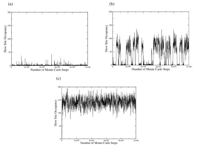
Figure 3: Graphs showing the number of particles on the slow site against time for $\lambda=4$, $p=0.2$ with $M=1000$, obtained via Monte Carlo simulation. (a) System is at $\varphi=0.29$, between expected critical density, in this case $0.25$, and maximum of the overshoot. This is an extension of the fluid phase. (b) System is at $\varphi=0.34$, just past the maximum of the overshoot. This is the coexistence region, a small condensate is seen to appear intermittently, but is not stable over long periods of time. (c) System is at $\varphi=0.40$, beyond the ‘end’ of the overshoot region where the current is approaching its expected maximum value $v=p$. Here the large pile of particles at the slow site is stable and the system is in the condensed phase.

Of course, on a finite system, strictly one cannot identify thermodynamic phases. However, it is useful to think of putative phases emerging in large systems. In the following and Figure 3 ‘phase’ is often taken to mean such a putative phase.

Inspecting Figure 3 we see that the overshoot is initially an extension of the fluid phase (Figure 3a); up to the maximum of $v$ the system is still in the fluid phase. At the maximum a condensate begins to emerge on the slow site. In the range of densities just beyond the maximum of the overshoot the emergent condensate appears intermittently, but is not stable over long time periods (Figure 3b). We interpret this as ‘coexistence’ between the fluid and condensed phases, i. e. at any given time the system is in one or the other. Eventually this coexistence gives way to a clear condensate as $v$ drops back down to its predicted maximum value of $p$ (Figure 3c).

Having established what takes place in the overshoot region, we proceed in the next section to give an analytical account for this effect working within the canonical ensemble.

V Canonical analysis

The SDS detailed in (12, 13), has a convenient property in that the canonical normalisation, $\mathrm{Z}(M,L)$ (3), can be reduced to a single sum. This makes it possible to analyse the model directly within the canonical ensemble.

The form that $\mathrm{Z}(M,L)$ takes for the SDS model is

$$\mathrm{Z}(M,L)=\sum_{n=0}^{L}p^{-n}\frac{n!}{(1+\lambda)_{n}}\binom{L+M-n-2}{M-2}\;.$$ (43)

Here we have simply inserted the $\mathrm{f}_{\mu}$ (14,15) into the general expression for $\mathrm{Z}(M,L)$ (3). The simple form of the hopping rates for sites $\mu>1$ (13) allows the sum over $n_{2}\dots n_{M}$ to be performed easily, yielding the combinatoric factor which comes from the delta function in (3). We also re-label $n_{1}$ as $n$ for convenience.

The normalisation is the sum over all un-normalised probabilities of occupancies of the sites. This means that the magnitude of the $n^{\mathrm{th}}$ term in the sum (43) is proportional to the probability of the slow site having occupancy $n$. Thus if $\mathrm{Z}(M,L)$ is dominated by a maximum at low $n$, the corresponding system is in the fluid phase. Conversely, if $\mathrm{Z}(M,L)$ is dominated by a maximum at large $n$, the corresponding system is in the condensed phase. If there are two maxima of similar magnitudes we interpret this as phase coexistence. Thus investigating the maxima of this sum should furnish us with an explanation of the overshoot.

To investigate the maxima of this sum, we look for its stationary points, i. e. points where the ratio of two consecutive terms tends to one. Solving for these points gives a quadratic equation in $n$, the solutions of which are:

$$n=\frac{M}{2}\left[\varphi-\varphi_{\mathrm{c}}\right]+\frac{A}{2}{}\pm\frac{M}{2}\left[\left(\varphi-\varphi_{\mathrm{c}}\right)^{2}+\frac{1}{M}\left\{2\left(\varphi-\varphi_{\mathrm{c}}\right)A-4\lambda\varphi_{\mathrm{c}}(1+\varphi)\right\}\right.\\ \left.{}+\frac{1}{M^{2}}\left\{A^{2}+4\lambda\varphi_{\mathrm{c}}\right\}\right]^{\frac{1}{2}}\;,$$ (44)

where $\varphi_{\mathrm{c}}=p/(1-p)$ is the expected critical density and the constant $A=\varphi_{\mathrm{c}}/p+\varphi_{\mathrm{c}}(1+\lambda)$.

The nature of these turning points can be determined by considering the ratio of the first two terms and also of the last two in (43). In the following we also assume that $p\leq 1/(1+\lambda)$ for simplicity, although this turns out to make little difference to the overall picture.

First we note that the roots in (44) become real at a density $\varphi_{2}$ given by

$$\varphi_{2}=\frac{p}{1-p}-\frac{1}{M}\left(\frac{1+p(1-\lambda)}{1-p}\right)+\left[\frac{1}{M}\frac{4\lambda p}{(1-p)^{2}}-\frac{1}{M^{2}}\frac{8\lambda p}{(1-p)^{2}}\right]^{\frac{1}{2}}\;.$$ (45)

Thus on increasing the density from zero the profile of the terms in the sum goes through the sequence illustrated in Figure 4: (a) For $\varphi<\varphi_{2}$ there is a boundary maximum at $n=0$; (b) at $\varphi=\varphi_{2}$ a stationary point emerges; (c) for $\varphi>\varphi_{2}$ a maximum emerges at large $n$ in addition to the local maximum at $n=0$; (d) the maximum at large $n$ increases and dominates, with $n=0$ eventually becoming a boundary minimum.

Figure 4: Graphs showing the logarithm of the terms from the normalisation sum $\mathrm{Z}(M,L)$ (43), for a system of size $M=1000$, with $\lambda=4$ and $p=0.15$. (a) $L=200$ ($\varphi<\varphi_{2}$), boundary maximum at $n=0$, no turning points. (b) $L=233$ ($\varphi=\varphi_{2}$), boundary maximum at $n=0$ and stationary point at higher $n$. (c) $L=300$ ($\varphi>\varphi_{2}$), boundary maximum at $n=0$ with greater maximum at high $n$. (d) $L=500$ ($\varphi\gg\varphi_{2}$), boundary minimum at $n=0$ and maximum at high $n$.

We interpret this sequence as follows. At low density, $\varphi<\varphi_{2}$ there are no turning points in the physical region $0\leq n\leq L$, with $n$ real. Thus the values of $n$ near $n=0$ dominate and this corresponds to the fluid phase. If we were to consider the $M\to\infty$ limit of (45) we would obtain $\varphi_{2}=\varphi_{\mathrm{c}}$. However for $M$ finite, the square root part of (44) remains imaginary up to $\varphi_{2}>\varphi_{\mathrm{c}}$ and the system remains in the fluid phase until this point. Thus the maximum at high $n$ emerges beyond the expected critical density $\varphi_{\mathrm{c}}=p/(1-p)$ by an amount ${\cal O}(M^{-1/2})$:

$$\varphi_{2}=\frac{p}{1-p}+\frac{2}{1-p}\left(\frac{\lambda p}{M}\right)^{1/2}+{\cal O}(\frac{1}{M})\;.$$ (46)

When $\varphi$ is just greater than $\varphi_{2}$ we interpret the boundary maximum at $n=0$ and the turning point at large $n$ as coexisting fluid and condensed phases. Finally, for $\varphi$ much larger than $\varphi_{2}$ the maximum at high $n$ dominates and we interpret this as the condensed phase.

We expect that the maximum of the overshoot will be near to the point $\varphi_{2}$ as this is where a putative condensate can begin to form and reduce the current. We see that an amount ${\cal O}(M^{-1/2})$ beyond $\varphi_{\mathrm{c}}$ is consistent with the data from exact numerical calculation of the current (Figure 2). In fact, we compared the peak of the overshoot with $\varphi_{2}$ for systems of size $M=1000$ we found very good agreement for $\lambda\approx 1\dots 6$. Outwith this range we believe that further finite size effects are becoming important.

The form of $\mathrm{Z}(M,L)$, given in equation (43), also allows the behaviour of the current in the condensed phase to be analysed. One finds that the asymptotic behaviour of the current for large particle number (i. e. where the sum in (43) is dominated by a maximum at large $n$) is

$$v=p\left[1+\frac{1}{M}\frac{\lambda}{(\varphi-\varphi_{\mathrm{c}})}+{\cal O}\left(\frac{1}{M^{2}}\right)\right]\;.$$ (47)

Thus for $\lambda>0$ the current approaches its asymptotic value from above as $\varphi\to\infty$. It should be noted that the second term in the expansion is small only for $\varphi-\varphi_{\mathrm{c}}\gg\lambda/M$.

VI Discussion

In this work we have studied the condensation transitions of a ZRP with a single defect site, in both the grand canonical and canonical ensembles. Analysis in the grand canonical ensemble predicts the two different condensation mechanisms (A and B) discussed in Section II.3.1. For $\lambda>2$ mechanism A applies which predicts a finite size overshoot in the current. The approach of $v$ to its saturation value $p$ is $v/p=1+{\cal O}(\ln L/L)$. For $\lambda\leq 2$ mechanism B applies and there should be no overshoot.

However, simulations in the canonical ensemble reveal an overshoot for all $\lambda>0$; only for $\lambda=0$ do we see the expected mechanism B behaviour. Analysis within the canonical ensemble confirms this and predicts that for $\lambda>0$ the overshoot in the current peaks at a density $\varphi=\varphi_{\mathrm{c}}+{\cal O}(M^{-1/2})$. The approach of $v$ to its saturation value as particle number increases is $v/p=1+{\cal O}(1/L)$. Thus it is not clear to what extent the mechanisms A and B are relevant or well-defined within the canonical ensemble. Moreover, from the point of view of finite size critical behaviour, the two ensembles are not equivalent.

It would be interesting to further understand the finite size inequivalence of the ensembles. In order to shed some light on this one can follow a standard approach khuangbook ; BBJ ; BrazJPhysMRE to evaluating the canonical normalisation (3) in terms of the grand canonical partition function (5). We use the integral representation of the delta function to write the canonical normalisation as a contour integral in the complex plane

$$\mathrm{Z}(M,L)=\oint\frac{\mathrm{d}s}{2\pi i}s^{-L+1}{\cal Z}(s)\;.$$ (48)

Then for large system size and particle number, $M$ and $L$ respectively, this integral will be dominated by its saddle point, given by

$$\varphi=\frac{s}{M}\sum_{\mu=1}^{M}\frac{\mathrm{F}_{\mu}^{\prime}(s)}{\mathrm{F}_{\mu}(s)}\;,$$ (49)

where $\varphi$ is the particle density ($L/M$). This equation precisely recovers (10). However it must be borne in mind that (49) holds only when the saddle point of (48) is valid, i. e. when it dominates the integral (48). It would not be surprising for the saddle point to break down when it approaches the radius of convergence of ${\cal Z}(s)$ in a way that depends on system size, as in the analysis of (10) in section II.3. Further analysis of this phenomenon would be enlightening.

Finally it would be of interest to perform simulations within the grand canonical ensemble to confirm our analytical predictions. To do this one would introduce transitions whereby particles are created and annihilated with appropriate rates.

- (1) M. R. Evans, Braz. J. Phys. 30, 42 (2000)
- (2) O. J. O’Loan, M. R. Evans and M. E. Cates, Phys. Rev. E 58, 1404 (1998)
- (3) S. N. Majumdar, S. Krishnamurthy and M. Barma, Phys. Rev. Lett. 81, 3691-3694 (1998)
- (4) D. Chowdhury, L. Santen, A. Schadschneider, Physics Reports 329, 199 (2000)
- (5) F. Spitzer, Advances in Math. 5, 246 (1970)
- (6) S. Grosskinsky, G. M. Schütz and H. Spohn, J. Stat. Phys. 113, 389 (2003)
- (7) Y. Kafri, E. Levine, D. Mukamel, G. M. Schütz and J. Török, Phys. Rev. Lett. 89, 035702, (2002)
- (8) M. R. Evans, Europhys. Lett. 36, 13 (1996)
- (9) J. Krug and P. A. Ferrari, J. Phys. A 29, L465 (1996)
- (10) M. R. Evans, J. Phys. A 30, 5669 (1997)
- (11) R. Barlovic, L. Santen, A. Schadschneider and M. Schreckenberg, Eur. Phys. J. B 5, 793, (1998)
- (12) K. Huang, Statistical Mechanics, (John Wiley and Sons, 1987)
- (13) Y. Kafri, D. Mukamel and L. Peliti, Eur. Phys. J. B 27, 135 (2002)
- (14) G. E. Andrews, R. Askey and P. Roy, Ed. G. -C. Rota, Special Functions (Encyclopedia of Mathematics and its Applications vol. 71), (Cambridge University Press, 1999)
- (15) P. Bialas, Z. Burda and D. Johnston, Nucl. Phys. B 493, 505 (1997)