Nambu-Goldstone Mode in a Rotating Dilute Bose-Einstein Condensate

Abstract

The Nambu-Goldstone mode, associated with vortex nucleation in a harmonically confined, two-dimensional dilute Bose-Einstein condensate, is identified with the lowest-lying envelope of octupole-mode branches, which are separated from each other by the admixture of quadrupolar excitations. As the vortex approaches the center of the condensate and the system’s axisymmetry is restored, the Nambu-Goldstone mode becomes massive due to its coupling to higher rotational bands.

One of the unique features of a gaseous Bose-Einstein condensate (BEC) is the fine tunability of interatomic interactions due to the Feshbach resonance MIT ; JILA . This degree of freedom can be utilized to explore some unique features of a rotating BEC by making the strength of interaction close to zero; then as the angular momentum (AM), $L$, of the system increases, the low-lying states of the BEC in a harmonic potential become quasi-degenerate WGS ; Mottelson and hence highly susceptible to symmetry-breaking perturbations. Such high susceptibility is considered to be the origin of vortex nucleation. Both experiments Madison and mean-field theories Butts ; Tsubota have demonstrated that as $L$ increases, vortices enter the system from the outskirts of the BEC by spontaneously breaking the system’s axisymmetry. Associated with this symmetry breaking must be a Nambu-Goldstone mode (NGM) which, however, has been elusive. This paper reveals the NGM using many-body theory and shows that this mode becomes massive as the vortex approaches the center of BEC at which point the axisymmetry of the system is restored.

We consider a system of $N$ identical bosons, each with mass $M$, that undergo contact interactions and are confined in a two-dimensional harmonic potential with frequency $\omega$. Throughout this paper, we measure the length, energy, and AM in units of $(\hbar/M\omega)^{1/2}$, $\hbar\omega$, and $\hbar$, respectively. The single-particle and interaction Hamiltonians are then given by $H_{0}=\sum_{j=1}^{N}(-2\partial^{2}/\partial z_{j}\partial z_{j}^{*}+|z_{j}|^{2}/2)$ and $V=2\pi g\sum_{j\neq k}\delta(z_{j}-z_{k})$, where $z_{j}\equiv x_{j}+iy_{j}$ is the complex coordinate of the $j$-th particle and $g$ gives the ratio of the mean-field interaction energy per particle to $\hbar\omega$. When $g\ll 1$, it is legitimate to restrict the Hilbert space to that spanned by the basis functions $\phi_{m}(z)=(z^{m}/\sqrt{\pi m!})\,e^{-|z|^{2}/2}\ (m=0,1,2,\cdots)$, where $m$ is the AM quantum number. In this “lowest-Landau-level” approximation, the field operator is expanded as $\hat{\Psi}(z)=\sum_{m=0}^{\infty}\hat{b}_{m}\phi_{m}(z)$, where $\hat{b}_{m}$ is the annihilation operator of a boson with AM $m$. The second-quantized form of $V$ then reads BP $\hat{V}=g\sum_{m_{1},\cdots,m_{4}}V_{m_{1},\cdots,m_{4}}\hat{b}_{m_{1}}^{\dagger}\hat{b}_{m_{2}}^{\dagger}\hat{b}_{m_{3}}\hat{b}_{m_{4}}$, where $V_{m_{1},\cdots,m_{4}}=\delta_{m_{1}+m_{2},m_{3}+m_{4}}(m_{1}+m_{2})!/(2^{m_{1}+m_{2}}\sqrt{m_{1}!m_{2}!m_{3}!m_{4}!})$. Since $\hat{H}_{0}=L+N$ is constant for given $L$ and $N$, the dynamics of the system is determined by $\hat{V}$ alone. The lowest-energy state of this system at a given $L$ is referred to as the yrast state, whose interaction energy is given for a repulsive case by $gN(N-1-L/2)$ BP ; SW . The trace of the yrast state viewed as a function of $L$ is called the yrast line. In the following we will measure the energy of the system from that of the yrast state.

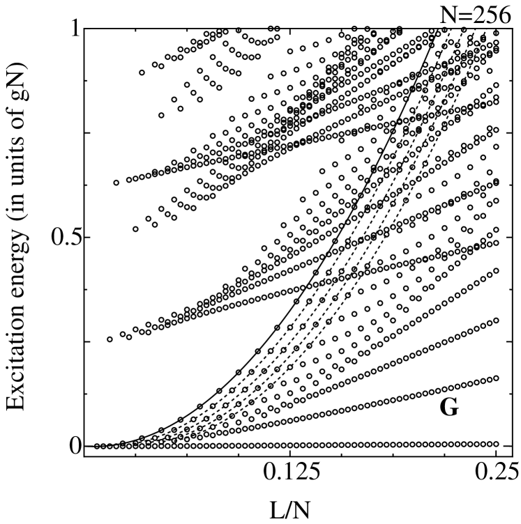
Figure 1: Nambu-Goldstone mode (labeled G) and its mass acquisition in a rotating BEC. The energy is measured from the yrast line (horizontal bottom line). The solid curve shows the branch that arises from octupole-mode excitations alone and is described by $(27g/34)n_{3}(n_{3}-1)$, where $n_{3}$ denotes the number of octupole-mode excitations. The solid and dotted curves are obtained from the least-squares fit of the data to quadratic polynomials. The dotted curves are displaced from the solid one by 2, 4, 6, 8 units of angular momentum. These shifts are caused by the admixture of quadrupole-mode excitations. The lowest-energy envelope of these branches constitutes the Nambu-Goldstone mode which acquires mass as $L$ increases, as evident from the curve labeled G. The excited states that involve the center-of-mass motion are not shown.

NGM in a rotating BEC–. The NGM should appear when the vortex is about to nucleate; that is, when the axisymmetry of the system is being broken. In this regime ($L\ll N$), the excitation spectrum is divided into two groups having different characters UN . One of them involves excitations whose energies are on the order of $gN$, and the other involves pairwise repulsive interactions between octupole modes with excitation energies given by $\hat{O}=(27g/34)\hat{b}_{3}^{\dagger}\hat{b}_{3}(\hat{b}_{3}^{\dagger}\hat{b}_{3}-1)$ UN . Because the energy scale ($\sim g$) of the latter group is smaller, by a factor of $1/N$, than that of the former one and hence vanishes in the thermodynamic limit, one might suspect that $\hat{O}$ is the NGM. However, this is not the case. We show that the NGM is the envelope of equally-spaced octupole-mode branches. The envelope is labeled G in Fig. 1, which is obtained by exact diagonalization of $\hat{V}$ for $N=256$. This beautiful structure was not found previously because it emerges only for large $N$ and for relatively large values of $L/N$ Note . In Fig. 1, octupole-mode branches are indicated by solid and dotted curves, which are equally spaced with $\Delta L=2$. We have confirmed that this spacing is caused by the admixture of one quadrupole-mode excitation.

For a mode to qualify as a NGM, it must meet three conditions. It must be massless, it must be associated with a broken symmetry, and it must play the role of restoring the broken symmetry. Because the G mode belongs to the second group discussed above, the excitation energy vanishes in the thermodynamic limit. Thus the first condition is met. Since the yrast states for $L\leq N$ are energetically degenerate under a rotation with angular velocity $\Omega=\frac{\partial E_{\rm tot}}{\partial L}=\omega(1-\frac{gN}{2})$, an axisymmetry breaking is expected to occur even for an infinitesimal, anisotropic symmetry-breaking perturbation. In fact, as the vortex enters the system, the axisymmetry is broken as seen in mean-field density profiles in Fig. 2 (a). Thus the second condition is met. The symmetry-restoring force is a correction to the mean-field result, so that many-body theory must be invoked to find out whether the third condition is met. We note that in exact diagonalization calculations the single-particle density-distribution function, $\rho({\bf r})=\langle\hat{\Psi}^{\dagger}({\bf r})\hat{\Psi}({\bf r})\rangle$, is isotropic [i.e., $\rho({\bf r})=\rho(|{\bf r}|)$] and is not suitable for studying the problem of axisymmetry breaking. The symmetry breaking can be studied with the conditional distribution function (CDF) cpf defined as $\rho({\bf r};{\bf r}_{0})=\frac{1}{\rho({\bf r}_{0})}\,\langle\hat{\Psi}^{\dagger}({\bf r})\hat{\Psi}^{\dagger}({\bf r}_{0})\hat{\Psi}({\bf r}_{0})\hat{\Psi}({\bf r})\rangle$, where ${\bf r}_{0}$ is the position of a test particle. In order to ensure that the back action of placing the test particle on the system is negligible, we take $|{\bf r}_{0}|=3$ which is well outside the condensate. We set ${\bf r}_{0}=(r_{0},0)$ without loss of generality. Expanding the CDF in terms of $\cos(m\theta)$, we have

$${\tilde{\rho}}({\bf r};{\bf r}_{0}) \equiv \frac{N}{N-1}\,\rho({\bf r};{\bf r}_{0})-\rho(|{\bf r}|)$$ (1)

$$= \sum_{m=0}^{\infty}C_{m}(r;|{\bf r}_{0}|)\,\frac{\cos(m\theta)}{\sqrt{\pi}},$$

where $r$ and $\theta$ are the polar coordinates of ${\bf r}$.

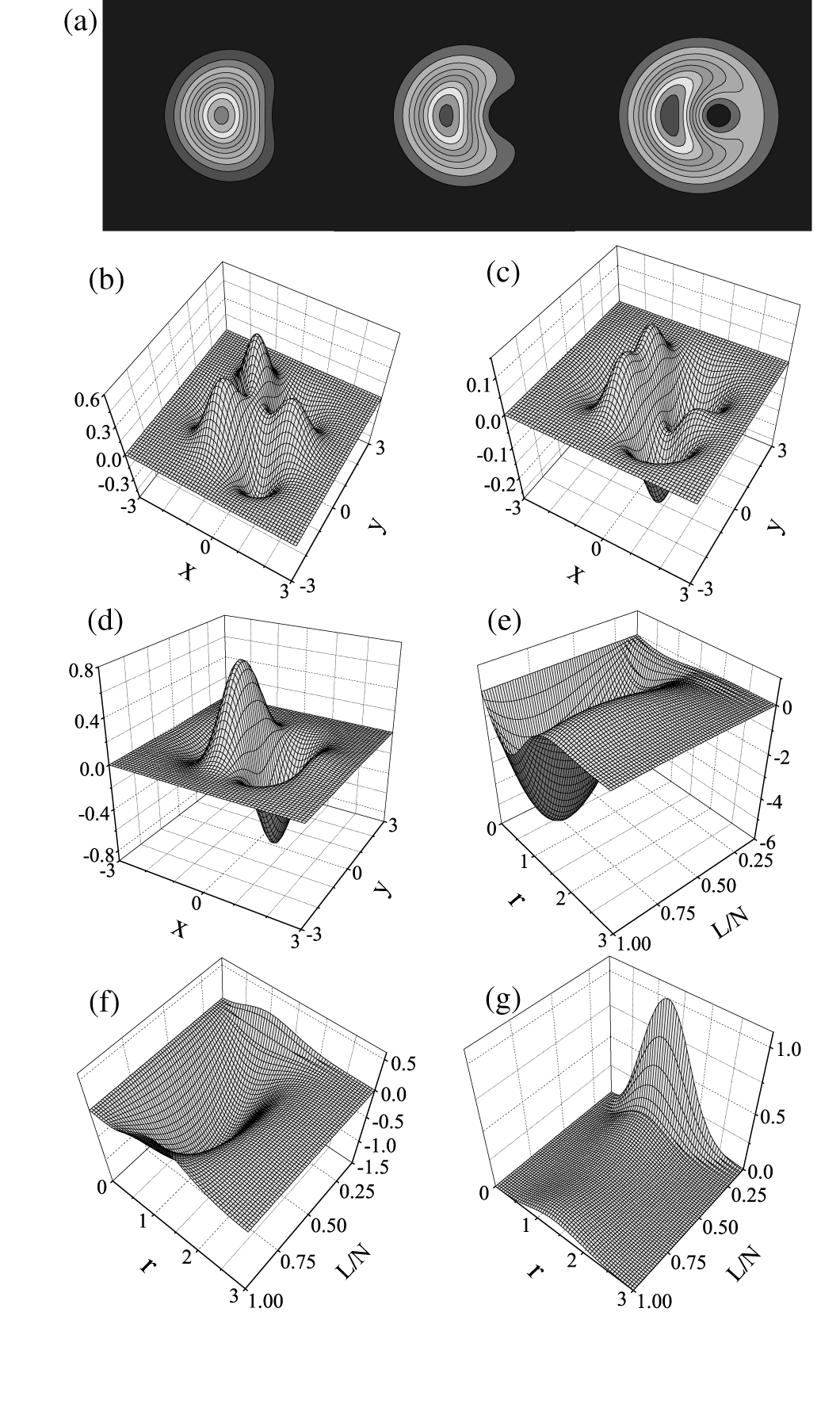
Figure 2: (a) Mean-field density profiles of BEC for $L/N=0.1,0.4,$ and 0.8. (b)-(c) Conditional distribution functions (CDFs) ${\tilde{\rho}}({\bf r};|{\bf r}_{0}|=3)$ defined in Eq. (1) for the quasi-degenerate lowest-lying excited state with $L=6$ (b) and $L=12$ (c). (d) CDF for the yrast state at $L=12$. (e)-(g) show expansion coefficients $C_{m}(r;|{\bf r}_{0}|=3)$ for $m=1,2$, and $3$, respectively, for the lowest-lying excited state for each $L$ satisfying $8\leq L\leq N=76$.

Figures 2(b) and (c) illustrate the CDF ${\tilde{\rho}}({\bf r};|{\bf r}_{0}|=3)$ for the lowest-lying excited states of 76 bosons with $L=6$ and $L=12$, respectively. The CDF in Fig. 2(b) features three-fold symmetry, reflecting the fact that the AM of this state is carried mostly by octupole-mode excitations. We also note that one of the peaks is located near the boundary of the condensate where the vortex comes in. This implies that the octupole-mode excitations compensate for the density depletion caused by the entrance of the vortex and thus plays the role of restoring the axisymmetry of the system. A further increase in $L$ is caused by quadrupole-mode excitations (see dotted curves in Fig. 1), so that the lowest-lying excited state gradually loses the character of three-fold symmetry, as illustrated in Fig. 2(c), and for larger $L$ the CDF eventually shows a dipole-like structure. On the other hand, Fig. 2(d) shows the CDF of the yrast state at $L=12$, featuring a dipole-like structure. The dipole-like distribution supports the entrance of the first vortex into the condensate by breaking the axisymmetry of the system.

Figures 2(e), (f), and (g) show the expansion coefficients $C_{m}(r;|{\bf r}_{0}|=3)$ in Eq. (1) for $m=1$, 2, and 3, respectively, for the lowest-lying excited states, which are constituting the G branch in Fig. 1. We note that $C_{1}(r;|{\bf r}_{0}|=3)$ is negative with large magnitude around $r=1$ (i.e., around the periphery of the condensate), which suggests that this component is responsible for the invasion of the vortex. On the other hand, the signs of $C_{m}(r;|{\bf r}_{0}|=3)$ for $m=2$ and $m=3$ are positive for $L\ll N$, and their magnitudes are maximal around $r=1$. This suggests that these two modes cooperate with each other to counteract the density depletion caused by the entrance of a vortex, in agreement with what is stated above. We note that the amplitudes of $C_{2}$ and $C_{3}$ dwindle rapidly and that $C_{2}$ changes its sign when $L$ increases beyond the quasi-degenerate region. This, too, supports our claim that they constitute the NGM. We have confirmed that the signs of $C_{4}$ and $C_{5}$ are also positive, but that their magnitudes are negligible compared with that of $C_{3}$.

Mass Acquisition of the NGM–. Finally, we investigate the mechanism by which the NGM becomes massive as $L$ increases. To this end, we separate the coordinates into center-of-mass (COM) $z_{\rm c}=(1/N)\sum_{j=1}^{N}z_{j}$ and relative ones $u_{j}\equiv z_{j}-z_{\rm c}$, where $\sum_{i=1}^{N}u_{i}=0$. Accordingly, $H_{0}$ is decomposed into the COM part $H^{\rm com}=-(2/N)\partial^{2}/\partial z_{\rm c}\partial z_{\rm c}^{*}+N|z_{\rm c}|^{2}/2$ and the relative part $H^{\rm rel}=(2/N)\sum_{j,k=1}^{N-1}(1-N\delta_{jk})\partial^{2}/\partial u_{j}\partial u_{k}^{*}+\sum_{j=1}^{N}|u_{j}|^{2}/2$. The total Hamiltonian is thus decomposed into the COM part $H^{\rm com}$ and the relative part $H^{\rm rel}+V$, where $V=2\pi g\sum_{j\neq k}\delta(u_{j}-u_{k})$. Therefore, a many-body wave function is separated into their counterparts: $\Psi(z_{1},z_{2},\cdots,z_{N})=\Psi^{\rm com}(z_{\rm c})\Psi^{\rm rel}(u_{1},u_{2},\cdots,u_{N-1})$. In what follows, we will ignore the COM part because it is decoupled from $V$.

We introduce a projection operator $e_{i}$, whose action is to eliminate those terms that contain the factor $u_{i}$ in the operand. For example, $e_{i}u_{j}=(1-\delta_{ij})u_{j},\ e_{i}u_{j}u_{k}=(1-\delta_{ij})(1-\delta_{ik})u_{j}u_{k}$, etc. As shown below, many-body wave functions can be constructed in a systematic way by appropriate operation of $e_{i}$ on the yrast-state wave function, which is known for $0\leq L\leq N$ to be $Y_{L}=\sum_{1\leq i_{1}<\cdots<i_{L}\leq N}u_{i_{1}}\cdots u_{i_{L}}$ BP . The low-lying excitations of interacting Bose systems are collective in nature Mottelson ; we claim that the main features (i.e., a large energy gap and almost linear rotational bands) of the excitation spectrum arise from a particular set of coupled collective excitations generated by operators $P_{m}=\sum_{i=1}^{N}u_{i}^{m}e_{i}$  ($m=0,1,\cdots$). These operators are analogous to Mottelson’s multipolar operators $Q_{m}\propto\sum_{i}z_{i}^{m}$ Mottelson but differ in that $z_{i}$ is replaced by $u_{i}$ and in that the projection operator $e_{i}$ is incorporated. Both of these modifications are essential for identifying an invariant subspace spanned by the yrast states and for constructing upon it the desired many-body excited states.

We consider a linear superposition of the states $M_{L}^{(m)}\equiv P_{m}Y_{L-m}$  ($m=3,4,\cdots,L$), where $M_{L}^{(m)}$ describes an excitation in which one particle carries AM $m$ and $L-m$ particles each carry a unit AM, for

$$M_{L}^{(m)}=\sum_{i_{1}<\cdots<i_{L-m+1}}\!\!\!\sum_{k=1}^{L-m+1}\!\!u_{i_{k}}^{m-1}\!\!\prod_{l=1}^{L-m+1}\!\!\!u_{i_{l}}.$$

The remaining $N-L+m-1$ particles carry no AM, and thus the condition $L\leq N+m-1$ must be met.

The transformation law of $M_{L}^{(m)}$ under the application of $V$ can be obtained as follows. The application of $2\pi\delta(u_{i}-u_{j})$ on $M_{L}^{(m)}$ gives

$$\!\!\!\!\!\!\!\!2\pi\delta(u_{i}-u_{j})M_{L}^{(m)}=M_{L}^{(m)}+\frac{(u_{i}-u_{j})^{2}}{4}e_{i}e_{j}M_{L-2}^{(m)}$$

$$\!\!\!\!\!\!\!\!+\left[\frac{(u_{i}+u_{j})^{m}}{2^{m-1}}-(u_{i}^{m}+u_{j}^{m})\right]e_{i}e_{j}Y_{L-m}$$

$$\!\!\!\!\!\!\!\!+\left[\frac{(u_{i}+u_{j})^{m+1}}{2^{m}}-(u_{i}^{m}u_{j}+u_{i}u_{j}^{m})\right]e_{i}e_{j}Y_{L-m-1}.$$ (2)

Summing both sides of this equation over $i$ and $j(\neq i)$, we obtain for $m\geq 3$

$$\!\!\!\!\tilde{V}M_{L}^{(m)}=\left\{(m+2^{3-m}-4)N+[2^{2-m}(m-1)+1]\right.$$

$$\left.\!\!\!\!\times(L-m)+4(1-2^{1-m})\right\}M_{L}^{(m)}/2-(1-2^{2-m})$$

$$\!\!\!\!\times(N-L+m)M_{L}^{(m+1)}/2+2^{2-m}m(L-m+1)$$

$$\!\!\!\!\!\times M_{L}^{(m-1)}+R_{m+1}+\theta(m\geq 4)R_{m},$$ (3)

where $\tilde{V}\equiv V-N(N-1-L/2)$ and

$$R_{m}=2^{1-m}\sum_{k=2}^{m-2}\frac{m!}{k!(m-k)!}P_{m-k}M_{L-m+k}^{(k)}.$$ (4)

Equation (3), together with (4), is the desired recursion relation. We see that each mode described by $M^{(m)}_{L}$ is coupled with other modes $M^{(k)}_{L}$ with $k=3,4,\cdots,m-1$, and $k=m+1$. Since the coefficient of $M^{(m+1)}_{L}$ in Eq. (3) includes a factor $N-L+m$ , the weight of this term decreases monotonically with increasing $L$. By introducing the truncation approximation discussed below and ignoring contributions from higher-order terms such as $M_{l}^{(l)}M_{L-l}^{(m)}$, we obtain a closed set of linear equations that can be solved easily even for a large value of $m$. It turns out that to quantitatively reproduce the G mode labeled in Fig. 1, we must take into account $m$ up to a relatively large value, such as 7, because higher rotational bands couple strongly to the G mode, as discussed below. Writing Eq. (3) explicitly for $m=3,4$, and $5$, we obtain

$$\tilde{V}M_{L}^{(3)} = (L-\frac{9}{4})M_{L}^{(3)}-\frac{N-L+3}{4}M_{L}^{(4)}$$

$$-\frac{3}{4}L(L-2)Y_{L},$$

$$\tilde{V}M_{L}^{(4)} = -\frac{L}{4}M_{L}^{(3)}+\frac{2N+7L-24}{8}M_{L}^{(4)}$$

$$-\frac{3}{8}(N-L+4)M_{L}^{(5)}+\frac{3}{4}L(L-2)Y_{L},$$

$$\tilde{V}M_{L}^{(5)} = -\frac{5}{8}(L-3)M_{L}^{(3)}-\frac{5}{16}(L-2)M_{L}^{(4)}$$ (5)

$$+\frac{10N+12L-55}{16}M_{L}^{(5)}$$

$$-\frac{7}{16}(N-L+5)M_{L}^{(6)},$$

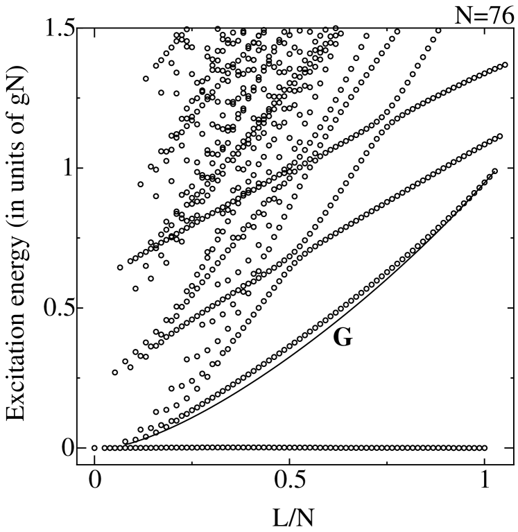
Figure 3: Comparison between the excitation energy of the G mode obtained by solving a set of linearized equations for $m=3,4,\cdots,7$ (solid curve) and those obtained by the exact diagonalization of the Hamiltonian (open circles). The energy is measured from the yrast state, which corresponds to the horizontal bottom line.

We note that the diagonal coefficients of $M_{L}^{(m)}$ in Eq. (5), are $(2N+7L)/8$ and $(5N+6L)/8$ for $m=4$ and $5$, respectively, and that they already reproduce rather well the almost linear spectra in Fig. 3. We refer to these as higher rotational bands. We also note the coupling of $M_{L}^{(m)}$ ($m\geq 4$) to $M_{L}^{(3)}$ becomes very strong, on the order of $O(N)$, near $L\sim N$. To reproduce the lowest-lying branch consisting mainly of $M_{L}^{(3)}$, we have to solve the coupled equations for $m=3,4,\cdots$. The solid curve in Fig. 3 shows the lowest excitation energy obtained by solving the above closed set of equations. It matches the G mode rather well.

In conclusion, we investigated the Nambu-Goldstone mode (NGM) of a rotating BEC associated with axisymmetry breaking due to vortex nucleation, and identified this mode with the lowest-lying envelope comprised of octupole branches that are equidistantly displaced by the admixture of quadrupole excitations. We found that as the angular momentum of the system increases, the NGM acquires mass due to its strong coupling to higher rotational bands.

References

• (1) S. Inouye, et al., Nature 392, 151 (1998).
• (2) S.L. Cornish, et al., Phys. Rev. Lett. 85, 1795 (2000).
• (3) N.K. Wilkin, et al., Phys. Rev. Lett. 80, 2265 (1998).
• (4) B. Mottelson, Phys. Rev. Lett. 83, 2695 (1999).
• (5) K. W. Madison, et al., Phys. Rev. Lett. 84, 806 (2000).
• (6) D. A. Butts and D. S. Rokhsar, Nature 397, 327 (1999).
• (7) M. Tsubota, et al., Phys. Rev. A 65, 023603 (2002).
• (8) G.F. Bertsch and T. Papenbrock, Phys. Rev. Lett. 83, 5412 (1999).
• (9) R.A. Smith and N.K. Wilkin, Phys. Rev. A 62, 61602 (2000); T. Papenbrock and G.F. Bertsch, ibid. 63, 023616 (2001).
• (10) T. Nakajima and M. Ueda, Phys. Rev. A 63, 043610 (2001); M. Ueda and T. Nakajima, ibid. 64, 063609 (2001); G.M. Kavoulakis, et al., ibid. 62, 063605 (2000); G.M. Kavoulakis, et al., ibid. 63, 055602 (2001); V. Bardek, et al., ibid. 64, 015603 (2001); V. Bardek and S. Meljanac, ibid. 65, 013602 (2002).
• (11) In a previous paper [T. Nakajima and M. Ueda, Phys. Rev. Lett. 91, 140401 (2003)], we reported the results of similar exact diagonalization calculations for $N=25$. However, this size is too small to reveal a quasi-degenerate spectrum on the order of $g$ so that we can distinguish the NGM from the yrast line. On the other hand, if we restrict $L$ as $L\ll N$, we can perform exact diagonalization calculations for a much larger $N$, say, $N=10000$, but then we are not able to cover $L$ up to $L/N\sim 0.1$, which is necessary in order to investigate how the NGM becomes massive with increasing $L$.
• (12) X.J. Liu, et al., Phys. Rev. Lett. 87, 030404 (2001).