Evaluation of Decoherence for Quantum Control and Computing

Abstract

Different approaches in quantifying environmentally-induced decoherence are considered. We identify a measure of decoherence, derived from the density matrix of the system of interest, that quantifies the environmentally induced error, i.e., deviation from the ideal isolated-system dynamics. This measure can be shown to have several useful features. Its behavior as a function of time has no dependence on the initial conditions, and is expected to be insensitive to the internal dynamical time scales of the system, thus only probing the decoherence-related time dependence. For a spin-boson model—a prototype of a qubit interacting with environment—we also demonstrate the property of additivity: in the regime of the onset of decoherence, the sum of the individual qubit error measures provides an estimate of the error for a several-qubit system, even if the qubits are entangled, as expected in quantum-computing applications. This makes it possible to estimate decoherence for several-qubits quantum computer gate designs for which explicit calculations are exceedingly difficult.

I Introduction

Dynamics of open quantum systems has increasingly attracted open ; CL ; Chakravarty ; Grabert ; vanKampen the attention of the community of scientists in diverse fields, working on realizations of quantum information processing. Recent interest in quantum computing has stimulated studies nonMarkov ; Anastopoulos ; Ford ; Braun ; Lewis ; Wang ; Lutz ; Khaetskii ; OConnell ; Strunz ; Haake ; PMV ; short ; Privman of environmental effects that cause small deviations from the isolated-system quantum dynamics. To perform large-scale quantum computation, environment-induced relaxation/decoherence effects during each short time interval of “quantum-gate” functions must be kept below a certain threshold in order to allow fault-tolerant quantum error correction qec ; Steane ; Bennett ; Calderbank ; SteanePRA ; Aharonov ; Gottesman ; Knill . The reduced density matrix of the quantum system, with the environment traced out, is usually evaluated within some approximation scheme, e.g., apscheme ; SPIE ; Zurek ; Shnirman . In this work, we focus on an additive measure of the deviation of the density matrix of a several-qubit system from the “ideal” density matrix of the system norm ; dd ; addnorm . The latter would describe the “ideal” dynamics, i.e., the system completely isolated from the environment. For a spin-boson model of a single two-state system (a qubit), this measure is calculated explicitly for the environment modeled as a bath of harmonic modes Caldeira , e.g., phonons or photons. We also establish that for a several-qubit quantum system, the introduced measure of decoherence is approximately additive for the time scales of interest, i.e., for short “gate function” times. The fact that this measure can be evaluated by summing up the deviation measures of the constituent qubits, which can be, in general, entangled, allows to avoid lengthy, tedious, and in most cases, intractable, many-body calculations. This new short-time additivity property is reminiscent of the approximate additivity expected for relaxation rates of exponential approach to equilibrium at large times, though the two properties are not related.

Let us briefly outline the commonly accepted scheme for implementing quantum algorithms in physical systems. The input data are encoded into the quantum states of several separated two-level systems (qubits). Then, their evolution is controlled by a Hamiltonian consisting of single-qubit operators and of two-qubit interaction terms Lloyd ; Barenco . Parameters of the Hamiltonian can be varied (controlled) externally to implement a given algorithm. In most quantum computer proposals Lloyd ; Barenco ; Lloyd2 ; Turchette ; Cirac ; Ekert ; Kventsel ; Kane ; Loss ; Imamoglu ; Rossi ; Nakamura ; Tanamoto ; Platzman ; Sanders ; Burkard ; Vrijen ; Fedichkin ; Bandyopadhyay ; Larionov this control is achieved by changing local electromagnetic fields around the qubits. Of course, this ideal model does not include the influence of the environment on the computation, which necessitates quantum error correction. The latter involves inevitably the implementation of non-unitary measurement-type operations qec ; Steane ; Bennett ; Calderbank ; SteanePRA ; Aharonov ; Gottesman ; Knill and cannot be described as Hamiltonian-governed dynamics of a closed system.

To study the effect of the environment, one needs to choose a suitable model for the environmental and its coupling to the system of interest. The accepted approach to evaluate environmentally induced decoherence involves a model in which each qubit is coupled to a bath of environmental modes Caldeira . The reduced density matrix of the system, with the bath modes traced out, then describes the time-dependence of the system evolution nonMarkov ; Anastopoulos ; Ford ; Braun ; Lewis ; Wang ; Lutz ; Khaetskii ; OConnell ; Strunz ; Haake ; PMV ; Markov ; Louisell ; Abragam ; Blum ; apscheme ; SPIE ; Zurek ; Shnirman . Due to the interaction with the environment, after each computational cycle the state of the qubits will deviate slightly from the ideal state. The deviation accumulates at each cycle, so that large-scale quantum computation is not possible without performing fault-tolerant error correction schemes qec ; Steane ; Bennett ; Calderbank ; SteanePRA ; Aharonov ; Gottesman ; Knill ; Kitaev ; Kitaev2 ; Kitaev3 . These schemes require the environmentally induced decoherence of the quantum state in one cycle to be below some threshold. The value of threshold, defined for uncorrelated single qubit error rates, was estimated Preskill ; DiVincenzo to be between $10^{-6}$ and $10^{-4}$.

To study decoherence for a given system, one should first obtain the evolution of its density matrix. This can be done by using various approximations nonMarkov ; Anastopoulos ; Ford ; Braun ; Lewis ; Wang ; Lutz ; Khaetskii ; OConnell ; Strunz ; Haake ; PMV ; short ; Markov ; Louisell ; Abragam ; Blum ; apscheme ; SPIE ; Zurek ; Shnirman . During each computational step the Hamiltonian of the studied system is usually considered to be constant. The most familiar are the Markovian-type approximations Markov ; Louisell ; Abragam ; Blum , used to evaluate approach to the thermal state at large times. It has been pointed out recently that these approximations are not suitable for quantum computing purposes because they are usually not valid vanKampen ; short at low temperatures and for short cycle times of quantum computation. Several non-Markovian approaches nonMarkov ; Anastopoulos ; Ford ; Braun ; Lewis ; Wang ; Lutz ; Khaetskii ; OConnell ; Strunz ; Haake ; PMV ; short ; Privman ; apscheme ; SPIE ; Zurek have been developed to evaluate the short-time dynamics of open quantum systems.

When one tries to study decoherence of several-qubit systems, additional difficulties should be taken into account. Namely, one has to consider the degree to which noisy environments of different qubits are correlated Storcz . For example, if all constituent qubits are effectively immersed in the same bath, then there is a way to reduce decoherence for this group of qubits without error correction algorithms. The reduction of error rate can be achieved by encoding the state of one logical qubit in a decoherence free subspace of the states of several physical qubits Palma ; DFS ; Zanardi ; Lidar . Therefore, in a large scale quantum information processor consisting of many thousands of qubits, it is more appropriate to consider qubits immersed in distinct baths, because these errors represent the “worst case scenario” that necessitates error-correction.

After obtaining the density matrix $\rho(t)$ for a single- or few-qubit system evaluated in some approximation, we have to compare it to the ideal density matrix $\rho^{(i)}(t)$ corresponding to quantum algorithm without environmental influences. It is convenient to define some measure of decoherence to compare with the fault-tolerance criteria qec ; Steane ; Bennett ; Calderbank ; SteanePRA ; Aharonov ; Gottesman ; Knill . It is desirable to have the measure nonnegative, and vanishing if and only if the system evolves in complete isolation. Since explicit calculations beyond one or very few qubits are exceedingly difficult, it would be also useful to find a measure which is additive (or at least sub-additive), i.e., the measure of decoherence, $D$ of a composite system will be the sum (or not greater than the sum) of the measures of decoherence, $D_{j}$, of its subsystems,

$$D\leq\sum_{j}D_{j}.$$ (1)

In this work, we identify a measure of decoherence which has these desirable properties. In Section II, we give an overview of different methods for quantifying decoherence. We note that in some cases these numerical measures have oscillations on the time scales of the internal system frequencies, which do not reflect the nature of decoherence. Therefore, in the next Section III we define the norm that is subadditive for non-interacting initially unentangled qubits and in most cases is a monotonic function of time. To establish stronger properties of subadditivity of this norm even for initially entangled qubits we will use a more sophisticated diamond norm. It is defined in Section IV. Relation between these norms and conditions for subadditivity for initially entangled qubits are also discussed. In Section V, we consider a specific model of a qubit interacting with a bosonic bath of environmental modes. For two types of interaction we explicitly obtain norms $D$ and $K$ for one qubit and prove asymptotic additivity for short times, $t$,

$$D(t)=\sum_{j}D_{j}(t)+o\left(\sum_{j}D_{j}(t)\right).$$ (2)

This result should apply as a good approximation up to intermediate, inverse-system-energy-gap times short , and it is consistent with the recent finding Dalton that at short times decoherence of a trapped-ion quantum computer scales approximately linearly with the number of qubits.

II Different Approaches to Quantifying Decoherence

Typically, the total Hamiltonian of an open quantum system interacting with environment has the form

$$H=H_{S}+H_{B}+H_{I},$$ (3)

where $H_{S}$ is the internal system Hamiltonian, $H_{B}$ is the Hamiltonian of the environment (bath), $H_{I}$ is the system-bath interaction Hamiltonian. Over gate-function cycles, and between them, the terms in $H$ will be considered constant norm ; dd . Therefore, the overall density matrix $R(t)$ of the system and bath evolves according to

$$R(t)=e^{-iHt}R(0)e^{iHt}.$$ (4)

Here and in the following we use the convention $\hbar=1$.

Usually the initial density matrix is assumed Markov ; Louisell ; Abragam ; Blum to be a direct product of the initial density matrix of the system, $\rho(0)$, and the thermalized density matrix of the bath, $\Theta$,

$$R(0)=\rho(0){\raise 2.0pt\hbox{$\scriptscriptstyle{\otimes}$}}\Theta.$$ (5)

The reduced density matrix of the system is obtained by tracing out the bath modes,

$$\rho(t)={\rm Tr}_{\,B}\,R(t).$$ (6)

Usually the environment is assumed to be a large macroscopic system in thermal equilibrium at temperature $T$. Interaction with it leads to thermalization of the quantum system, so that the reduced density matrix at large times approaches

$$\rho\to\frac{{{e^{-\beta H_{S}}}}}{{{{\rm Tr}_{\,S}\left(e^{-\beta H_{S}}\right)}}},\qquad{\rm as}\;\;t\to\infty,$$ (7)

where $\beta=1/k_{B}T$. Markovian type approximations which are used to quantify this process yield exponential decay of the density matrix elements in the energy basis of the Hamiltonian $H_{S}$ Markov ; Louisell ; Abragam ; Blum ,

$$\rho_{nn}(t)-\rho_{nn}(\infty)\propto e^{-t/T_{nn}},$$ (8)

$$\rho_{nm}(t)\propto e^{-t/T_{nm}}\qquad(n\neq m).$$ (9)

The shortest times among $T_{nn}$ and $T_{n\neq m}$ are identified as characteristic times of thermalization $T_{1}$ and decoherence $T_{2}$, respectively. Thermalization of the quantum system requires the energy exchange with the environment while decoherence can include other faster processes without energy exchange. Therefore, it is commonly believed Blum that $T_{2}$ is much shorter than $T_{1}$ for low-temparature, well isolated from the environment systems appropriate for quantum computing realizations. The shorter time $T_{2}$ can be compared with $T_{g}$ needed for elementary quantum gate functions Privman2 . The ratio $T_{g}/T_{2}$ must be small in order to satisfy fault-tolerance criteria Preskill ; DiVincenzo . However, since $T_{2}$ is a large-time asymptotic property, other measures, representative of the short-time, $t\ll T_{2}$, decoherence properties, are preferred for actual numerical evaluations short .

The exponential behavior of the density matrix elements inherent to the Markovian approximation is valid on the time scale which is much larger than the internal inverse-system-energy-gap times of the quantum system. To measure effects of decoherence on these time scales one can use the entropy Neumann ,

$$S(t)=-{\rm Tr}\left(\rho\ln\rho\right),$$ (10)

or the idempotency defect, called also the first order entropy Kim ; Zurek2 ; Zagur ,

$$s(t)=1-{\rm Tr}\left(\rho^{2}\right).$$ (11)

Both expressions are zero only if the quantum system density operator is a projector $\rho(0)=|\varphi\rangle\langle\varphi|$. Any deviation from a pure state leads to the increase in the value of both measures. Expressions (10, 11) provide numerical measure of the system “purity” which does not rely on preferred basis. However, entropy measures do not distinguish different pure states.

The next step in analyzing the effect of the interaction with the environment is to define the “ideal” (without interaction) density operator evolution according to

$$\rho^{(i)}(t)\equiv e^{-iH_{S}t}\rho(0)e^{iH_{S}t}.$$ (12)

One of the measures that characterizes decoherence in term of the difference between the “real” evolution, $\rho(t)$, and “ideal” one, $\rho^{(i)}$, is the fidelity Dalton ; Fidelity2 ,

$$F(t)={\rm Tr}_{\,S}\left[\,\rho^{(i)}(t)\,\rho(t)\,\right].$$ (13)

It is particularly useful when $\rho^{(i)}(t)$ remains a projection operator (pure state) for all times $t\geq 0$, because it then attains the maximum value of 1 only when $\rho(t)=\rho^{(i)}(t)$.

An alternative way to quantify the effect of the interaction with the bath norm , is to consider the deviation, $\sigma(t)$,

$$\sigma(t)=\rho(t)-\rho^{(i)}(t),$$ (14)

of the reduced density matrix from the ideal one. As numerical measures of decoherence one can use the operator norm $\left\|\sigma\right\|_{\lambda}$ or trace norm $\left\|\sigma\right\|_{\rm Tr}$. Both norms are standard in in the theory of linear operators Kato . For an arbitrary linear operator, $A$, these norms are defined as follows,

$$\left\|A\right\|_{\lambda}=\mathop{\sup}\limits_{\varphi\neq 0}\left({\frac{{\langle\varphi|A^{\dagger}A|\varphi\rangle}}{{\langle\varphi|\varphi\rangle}}}\right)^{1/2},$$ (15)

$$\left\|A\right\|_{\rm Tr}={\rm Tr}\,\sqrt{A^{\dagger}A}.$$ (16)

For a finite-dimensional Hermitian deviation operator (14) these definitions are equivalent to

$$\left\|\sigma\right\|_{\lambda}={\max_{i}}\left|{\lambda_{i}}\right|,$$ (17)

$$\left\|\sigma\right\|_{{\rm Tr}}=\sum\limits_{i}{\left|{\lambda_{i}}\right|},$$ (18)

where $\lambda_{i}$ are the eigenvalues of $\sigma$.

In the simplest case of a two-level system (qubit), the two norms are proportional to each other and given by

$$\left\|\sigma\right\|_{\lambda}=\sqrt{\left|{\sigma_{11}}\right|^{2}+\left|{\sigma_{12}}\right|^{2}}={\frac{1}{2}}\left\|\sigma\right\|_{{\rm Tr}}.$$ (19)

The deviation norm $\left\|\sigma\right\|_{\lambda}$ has the minimal value, 0, only for $\rho(t)=\rho^{(i)}(t)$ without any additional conditions.

Note that the measures $\left\|\sigma\right\|_{\lambda}$ and $\left\|\sigma\right\|_{\rm Tr}$ are not only functions of time, but also depend on the initial density operator $\rho(0)$. Due to decoherence, they will deviate from zero for $t>0$. However, their time-dependence will also contain oscillations at the frequencies of the internal system dynamics, as will be illustrated below for $\left\|\sigma\right\|_{\lambda}$; see addnorm ; norm and Fig. 1. In the next section we define the maximal deviation norm, $D(t)$, which is typically a monotonic function of time.

III The Maximal Deviation Norm

To characterize decoherence for an arbitrary initial state, pure or mixed, we propose to use the maximal norm, $D$, which is determined as an operator norm maximized over all the possible initial density matrices. For instance, we can define

$$D(t)=\sup_{\rho(0)}\bigg{(}\left\|\sigma(t,\rho(0))\right\|_{\lambda}\bigg{)}.$$ (20)

One can show that $0\leq D(t)\leq 1$. This measure of decoherence will typically increase monotonically from zero at $t=0$, saturating at large times at a value $D(\infty)\leq 1$. The definition of the maximal decoherence measure $D(t)$ looks rather complicated for a general multiqubit system. However, we will show that it can be evaluated in closed form for short times, appropriate for quantum computing, for a single-qubit (two-state) system. We then establish an approximate additivity that allows us to estimate $D(t)$ for several-qubit systems as well.

In the superoperator notation the evolution of the reduced density operator of the system (6) and the one for the ideal density matrix (12) can be formally expressed Kitaev ; Kitaev2 ; Kitaev3 in the following way

$$\rho(t)=T(t)\rho(0),$$ (21)

$$\rho^{(i)}(t)=T^{(i)}(t)\rho(0),$$ (22)

where $T$, $T^{(i)}$ are linear superoperators. In this notation the deviation can be expressed as

$$\sigma(t)=\left[T(t)-T^{(i)}(t)\right]\rho(0).$$ (23)

The initial density matrix can always be written in the following form,

$$\rho(0)=\sum_{j}p_{j}|\psi_{j}\rangle\langle\psi_{j}|,$$ (24)

where $\sum_{j}p_{j}=1$ and $0\leq p_{j}\leq 1$. Here the set of the wavefunctions $|\psi_{j}\rangle$ is not assumed to have any orthogonality properties. Then, we get

$$\sigma\left(t,\rho(0)\right)=\sum_{j}p_{j}\left[T(t)-T^{(i)}(t)\right]\left|\psi_{j}\right\rangle\left\langle\psi_{j}\right|.$$ (25)

The deviation norm can thus be bounded,

$$\|\sigma(t,\rho(0))\|_{\lambda}\leq\left\|\left[T(t)-T^{(i)}(t)\right]|\phi\rangle\langle\phi|\right\|_{\lambda}.$$ (26)

Here $|\phi\rangle$ is defined according to

$$\left\|\left[T-T^{(i)}\right]|\phi\rangle\langle\phi|\right\|_{\lambda}=\max_{j}\left\|\left[T-T^{(i)}\right]|\psi_{j}\rangle\langle\psi_{j}|\right\|_{\lambda}.$$

It transpires that for any initial density operator which is a statistical mixture, one can always find a density operator which is pure-state, $|\phi\rangle\langle\phi|$, such that $\|\sigma(t,\rho(0))\|_{\lambda}\leq\|\sigma(t,|\phi\rangle\langle\phi|)\|_{\lambda}$. Therefore, evaluation of the supremum over the initial density operators in order to find $D(t)$, see (20), one can done over only pure-state density operators.

Let us consider strategies of evaluation of $D(t)$ for a single qubit. We can parameterize $\rho(0)$ as

$$\rho(0)=U\left(\begin{array}[]{cc}P&0\\ 0&1-P\\ \end{array}\right)U^{\dagger},$$ (27)

where $0\leq P\leq 1$, and $U$ is an arbitrary $2\times 2$ unitary matrix,

$$U=\left(\begin{array}[]{cc}e^{i(\alpha+\gamma)}\cos\theta&e^{i(\alpha-\gamma)}\sin\theta\\ -e^{i(\gamma-\alpha)}\sin\theta&e^{-i(\alpha+\gamma)}\cos\theta\\ \end{array}\right).$$ (28)

Then, one should find a supremum of the norm of deviation (17) over all the possible real parameters $P$, $\alpha$, $\gamma$ and $\theta$. As shown above, it suffices to consider the density operator in the form of a projector and put $P=1$. Thus, one should search for the maximum over the remaining three real parameters $\alpha$, $\gamma$ and $\theta$.

Another parametrization of the pure-state density operators, $\rho(0)=|\phi\rangle\langle\phi|$, is to express an arbitrary wave function $|\phi\rangle=\sum_{j}(a_{j}+ib_{j})|j\rangle$ in some convenient ortonormal basis $|j\rangle$, where $j=1,\ldots,N$. For a two-level system,

$$\rho(0)=\left(\begin{array}[]{cc}a_{1}^{2}+b_{1}^{2}&(a_{1}+ib_{1})(a_{2}-ib_{2})\\ (a_{1}-ib_{1})(a_{2}+ib_{2})&a_{2}^{2}+b_{2}^{2}\\ \end{array}\right),$$ (29)

where the four real parameters $a_{j},b_{j}$, with $j=1,2$ satisfy $a_{1}^{2}+b_{1}^{2}+a_{2}^{2}+b_{2}^{2}=1$, so that the maximization is again over three independent real numbers. In the following sections, we will consider examples of evaluation of $D(t)$ for single-qubit systems.

In quantum computing, the error rates can be significantly reduced by using several physical qubits to encode each logical qubit DFS ; Zanardi ; Lidar . Therefore, even before active quantum error correction is incorporated qec ; Steane ; Bennett ; Calderbank ; SteanePRA ; Aharonov ; Gottesman ; Knill , evaluation of decoherence of several qubits is an important, but formidable task. Consider a system consisting of two initially unentangled subsystems $S_{1}$ and $S_{2}$, with decoherence norms $D_{S_{1}}$ and $D_{S_{2}}$, respectively. We denote the density matrix of the full system as $\rho_{S_{1}S_{2}}$ and its deviation as $\sigma_{S_{1}S_{2}}$, and use a similar notation with subscripts $S_{1}$ and $S_{2}$ for the two subsystems. If the evolution of system is governed by the “noninteracting” Hamiltonian of the form $H_{S_{1}S_{2}}=H_{S_{1}}+H_{S_{2}}$, where the terms $H_{S_{1}}$, $H_{S_{2}}$ act only on variables of the system $S_{1}$, $S_{2}$, respectively, then the overall norm $D_{S_{1}S_{2}}$ can be bounded by the sum of the norms $D_{S_{1}}$ and $D_{S_{2}}$,

$$D_{S_{1}S_{2}}^{\vphantom{(i)}}=\sup_{\rho(0)}\|\sigma_{S_{1}S_{2}}^{\vphantom{(i)}}\|_{\lambda}=\sup_{\rho(0)}\|\rho_{S_{1}S_{2}}^{\vphantom{(i)}}-\rho^{(i)}_{S_{1}S_{2}}\|_{\lambda}$$ (30)

$$=\sup_{\rho(0)}\|\rho_{S_{1}}^{\vphantom{(i)}}\!{\raise 2.0pt\hbox{$\scriptscriptstyle{\otimes}$}}\rho_{S_{2}}^{\vphantom{(i)}}\!-\rho_{S_{1}}^{(i)}{\raise 2.0pt\hbox{$\scriptscriptstyle{\otimes}$}}\rho_{S_{2}}^{(i)}\|_{\lambda}=\sup_{\rho(0)}\|\sigma_{S_{1}}^{\vphantom{(i)}}\!{\raise 2.0pt\hbox{$\scriptscriptstyle{\otimes}$}}\rho_{S_{2}}^{\vphantom{(i)}}\!+\rho_{S_{1}}^{(i)}{\raise 2.0pt\hbox{$\scriptscriptstyle{\otimes}$}}\sigma_{S_{2}}^{\vphantom{(i)}}\|_{\lambda}$$

Since the operator norm obeys the triangle inequality Kato

$$\|\sigma_{S_{1}}^{\vphantom{(i)}}\!{\raise 2.0pt\hbox{$\scriptscriptstyle{\otimes}$}}\rho_{S_{2}}^{\vphantom{(i)}}\!+\rho_{S_{1}}^{(i)}{\raise 2.0pt\hbox{$\scriptscriptstyle{\otimes}$}}\sigma_{S_{2}}^{\vphantom{(i)}}\|_{\lambda}\leq\|\sigma_{S_{1}}^{\vphantom{(i)}}\!{\raise 2.0pt\hbox{$\scriptscriptstyle{\otimes}$}}\rho_{S_{2}}^{\vphantom{(i)}}\!\|_{\lambda}+\|\rho_{S_{1}}^{(i)}{\raise 2.0pt\hbox{$\scriptscriptstyle{\otimes}$}}\sigma_{S_{2}}^{\vphantom{(i)}}\|_{\lambda},$$ (31)

we can estimate the last expression as

$$D_{S_{1}S_{2}}^{\vphantom{(i)}}=\sup_{\rho(0)}\|\sigma_{S_{1}}^{\vphantom{(i)}}\!{\raise 2.0pt\hbox{$\scriptscriptstyle{\otimes}$}}\rho_{S_{2}}^{\vphantom{(i)}}\!+\rho_{S_{1}}^{(i)}{\raise 2.0pt\hbox{$\scriptscriptstyle{\otimes}$}}\sigma_{S_{2}}^{\vphantom{(i)}}\|_{\lambda}\leq\sup_{\rho(0)}\|\sigma_{S_{1}}^{\vphantom{(i)}}{\raise 2.0pt\hbox{$\scriptscriptstyle{\otimes}$}}\rho_{S_{2}}^{\vphantom{(i)}}\|_{\lambda}+\sup_{\rho(0)}\|\rho_{S_{1}}^{(i)}{\raise 2.0pt\hbox{$\scriptscriptstyle{\otimes}$}}\sigma_{S_{2}}^{\vphantom{(i)}}\|_{\lambda}.$$ (32)

Each eigenvalue of the tensor product of two linear operators is formed as a pairwise product of eigenvalues of the two operators. Therefore, the operator norm of the tensor product of two operators is equal to product of their operator norms,

$$\|A_{1}{\raise 2.0pt\hbox{$\scriptscriptstyle{\otimes}$}}A_{2}\|_{\lambda}=\|A_{1}\|_{\lambda}\|A_{2}\|_{\lambda}.$$ (33)

We use this property and the fact that the eigenvalues of density matrices $\rho_{S_{1}},\rho_{S_{2}}$ are in $[0,1]$ to derive the estimate

$$D_{S_{1}S_{2}}^{\vphantom{(i)}}\leq\sup_{\rho_{S_{1}}(0)}\|\sigma_{S_{1}}^{\vphantom{(i)}}\|_{\lambda}+\sup_{\rho_{S_{2}}(0)}\|\sigma_{S_{2}}^{\vphantom{(i)}}\|_{\lambda}=D_{S_{1}}^{\vphantom{(i)}}+D_{S_{2}}^{\vphantom{(i)}}.$$ (34)

In general, initially unentangled qubits will remain nearly unentangled for short times, because they didn’t have enough time to interact. Therefore, the inequality

$$D\lesssim\sum_{q}D_{q},$$ (35)

is expected to provide a good approximate estimate for the norm of a multiqubit system $D$ in terms of the norms $D_{q}$ calculated in the space of each individual qubit, i.e., the measures of decoherence for the individual qubits can be considered approximately additive. For large times, the separate measures become of order 1, so such a bound is not useful. Instead, the rates of approach of various quantities to their asymptotic values are approximately additive in some cases.

In the rest of this work, we focus on the short-time and adiabatic (i.e., no energy exchange with the bath basis ) regimes, and establish a much stronger property: We prove the approximate additivity for the initially entangled qubits whose dynamics is governed by

$$H=\sum_{q}H_{q}=\sum_{q}\left(H_{Sq}+H_{Bq}+H_{Iq}\right),$$ (36)

where $H_{Sq}$ is the Hamiltonian of the $q$th qubit itself, $H_{Bq}$ is the Hamiltonian of the environment of the $q$th qubit, and $H_{Iq}$ is corresponding qubit-environment interaction. For this purpose, in the next section we consider a more complicated (for actual evaluation) diamond norm Kitaev ; Kitaev2 ; Kitaev3 , $K(t)$, as an auxiliary quantity used to establish the additivity of the more easily calculable operator norm $D(t)$.

IV The Diamond Norm

The establishment of the upper-bound estimate for the maximal deviation norm of a multiqubit system, involves several derivations. We bound this norm by the recently introduced (in the contexts of quantum computing) Kitaev ; Kitaev2 ; Kitaev3 diamond norm, $K(t)$. Actually, for single qubits, in several models the diamond norm can be expressed via the corresponding maximal deviation norm. At the same time, the diamond norm for the whole quantum system is bounded by sum of the norms of the constituent qubits by using a specific stability property of the diamond norm. The use of diamond norm was proposed by Kitaev Kitaev ; Kitaev2 ; Kitaev3 ,

$$K(t)=\|T-T^{(i)}\|_{\diamond}=\sup_{\varrho}\|\{[T-T^{(i)}]{\raise 2.0pt\hbox{$\scriptscriptstyle{\otimes}$}}I\}{\varrho}\|_{\rm Tr}.$$ (37)

The superoperators $T$, $T^{(i)}$ characterize the actual and ideal evolutions according to (21, 22), $I$ is the identity superoperator on a Hilbert space $G$ whose dimension is the same as that of the corresponding space of the superoperators $T$ and $T^{(i)}$, and $\varrho$ is an arbitrary density operator in the product space of twice the number of qubits.

The diamond norm has an important stability property, proved in Kitaev ; Kitaev2 ; Kitaev3 ,

$$\|T_{1}{\raise 2.0pt\hbox{$\scriptscriptstyle{\otimes}$}}T_{2}\|_{\diamond}=\|T_{1}\|_{\diamond}\|T_{2}\|_{\diamond},$$ (38)

which should be compared with (33). Note that (38) is a property of the evolution superoperators rather than that of the density operators: The importance of this difference will become obvious shortly.

Consider again a composite system consisting of the two subsystems $S_{1}$, $S_{2}$, with the noninteracting Hamiltonian

$$H_{S_{1}S_{2}}=H_{S_{1}}+H_{S_{2}}.$$ (39)

The evolution superoperator of the system will be

$$T_{S_{1}S_{2}}=T_{S_{1}}{\raise 2.0pt\hbox{$\scriptscriptstyle{\otimes}$}}T_{S_{2}},$$ (40)

and the ideal one

$$T_{S_{1}S_{2}}^{(i)}=T_{S_{1}}^{(i)}{\raise 2.0pt\hbox{$\scriptscriptstyle{\otimes}$}}T_{S_{2}}^{(i)}.$$ (41)

The diamond measure for the system can be expressed as

$$K_{S_{1}S_{2}}^{\vphantom{(i)}}=\|T_{S_{1}S_{2}}^{\vphantom{(i)}}-T_{S_{1}S_{2}}^{(i)}\|_{\diamond}=\|(T_{S_{1}}^{\vphantom{(i)}}-T_{S_{1}}^{(i)}){\raise 2.0pt\hbox{$\scriptscriptstyle{\otimes}$}}T_{S_{2}}^{\vphantom{(i)}}+T_{S_{1}}^{(i)}{\raise 2.0pt\hbox{$\scriptscriptstyle{\otimes}$}}(T_{S_{2}}^{\vphantom{(i)}}-T_{S_{2}}^{(i)})\|_{\diamond}$$

$$\leq\|(T_{S_{1}}^{\vphantom{(i)}}-T_{S_{1}}^{(i)}){\raise 2.0pt\hbox{$\scriptscriptstyle{\otimes}$}}T_{S_{2}}^{\vphantom{(i)}}\|_{\diamond}+\|T_{S_{1}}^{(i)}{\raise 2.0pt\hbox{$\scriptscriptstyle{\otimes}$}}(T_{S_{2}}^{\vphantom{(i)}}-T_{S_{2}}^{(i)})\|_{\diamond}.$$ (42)

By using the stability property (38), we get

$$K_{S_{1}S_{2}}^{\vphantom{(i)}}\leq\|(T_{S_{1}}^{\vphantom{(i)}}-T_{S_{1}}^{(i)}){\raise 2.0pt\hbox{$\scriptscriptstyle{\otimes}$}}T_{S_{2}}^{\vphantom{(i)}}\|_{\diamond}+\|T_{S_{1}}^{(i)}{\raise 2.0pt\hbox{$\scriptscriptstyle{\otimes}$}}(T_{S_{2}}^{\vphantom{(i)}}-T_{S_{2}}^{(i)})\|_{\diamond}=\|T_{S_{1}}^{\vphantom{(i)}}-T_{S_{1}}^{(i)}\|_{\diamond}\|T_{S_{2}}^{\vphantom{(i)}}\|_{\diamond}+$$

$$\|T_{S_{1}}^{(i)}\|_{\diamond}\|T_{S_{2}}^{\vphantom{(i)}}-T_{S_{2}}^{(i)}\|_{\diamond}=\|T_{S_{1}}^{\vphantom{(i)}}-T_{S_{1}}^{(i)}\|_{\diamond}+\|T_{S_{2}}^{\vphantom{(i)}}-T_{S_{2}}^{(i)}\|_{\diamond}=K_{S_{1}}^{\vphantom{(i)}}+K_{S_{2}}^{\vphantom{(i)}}.$$ (43)

The approximate inequality

$$K\lesssim\sum_{q}K_{q},$$ (44)

for the diamond norm $K(t)$ has thus the same form as for the norm $D(t)$, (35). Let us emphasize that both relations apply assuming that for short times the subsystem interactions, directly with each other or via their coupling to the bath modes, have had no significant effect. However, there is an important difference in that the relation for $D(t)$ further requires the subsystems to be initially unentangled. This restriction does not apply for the relation derived for $K(t)$. This property is particularly useful for quantum computing, the power of which is based on qubit entanglement. However, even in the simplest case of the diamond norm of one qubit, the calculations are extremely cumbersome. Therefore, the measure $D(t)$ is preferrable for actual calculations.

The two deviation-operator norms considered Section II are related by the following inequality

$$\left\|\sigma\right\|_{{\lambda}}\leq\frac{1}{2}\left\|\sigma\right\|_{{\rm Tr}}\leq 1.$$ (45)

Here the left-hand side follows from

$$\rm{Tr}\,\sigma=\sum_{j}\lambda_{j}=0.$$ (46)

It follows that the $\ell$th eigenvalue of the deviation operator $\sigma$ that has the maximum absolute value, $\lambda_{\ell}=\lambda_{\rm{max}}$, can be expressed as

$$\lambda_{\ell}=-\sum_{j\neq\ell}\lambda_{j}.$$ (47)

Therefore, we have

$$\left\|\sigma\right\|_{{\lambda}}=\frac{1}{2}\left(2|\lambda_{\ell}|\right)\leq\frac{1}{2}\left(|\lambda_{\ell}|+\sum_{j\neq\ell}|\lambda_{j}|\right)=\frac{1}{2}\left(\sum_{j}|\lambda_{j}|\right)=\frac{1}{2}\left\|\sigma\right\|_{\rm Tr}.$$ (48)

The right-hand side of (45) then also follows, because any density matrix has trace norm 1,

$$\|\sigma\|_{{\rm Tr}}=\|\rho-\rho^{(i)}\|_{{\rm Tr}}\leq\|\rho\|_{{\rm Tr}}+\|\rho^{(i)}\|_{{\rm Tr}}=2.$$ (49)

From the relation (49) it follows that

$$K(t)\leq 2.$$ (50)

By taking supremum of the both sides of the relation (48) we get

$$D(t)=\sup_{\rho(0)}\left\|\sigma\right\|_{{\lambda}}\leq\frac{1}{2}\sup_{\rho(0)}\left\|\sigma\right\|_{\rm Tr}\leq\frac{1}{2}K(t),$$ (51)

where the last step involves technical derivation details not reproduced here. In fact, in the following sections we show that for a single qubit, calculations within selected models actually give

$$D(t)=\frac{1}{2}K(t).$$ (52)

Since $D$ is generally bounded by (or equal to) $K/2$, it follows that the multiqubit norm $D$ is approximately bounded from above by the sum of the single-qubit norms even for the initially entangled qubits,

$$D(t)\leq\frac{1}{2}K(t)\lesssim\frac{1}{2}\sum_{q}K_{q}=\sum_{q}D_{q},$$ (53)

where $q$ labels the qubits.

V Decoherence in the Short-Time Approximation

Typically the environment, a large macroscopic system, is modelled by a bath of an infinite number of modes. Each mode is represented by its own Hamiltonian $M_{k}$,

$$H_{B}=\sum\limits_{k}\,M_{k}.$$ (54)

The interaction with the bath is often described by the coupling of its modes to Hermitian operator $\Lambda_{S}$ of the quantum system,

$$H_{I}=\Lambda_{S}\sum\limits_{k}\,J_{k}.$$ (55)

For a bosonic-mode heat bath Leggett we take

$$M_{k}=\omega_{k}a_{k}^{\dagger}a_{k}^{\vphantom{\dagger}},\quad J_{k}=g_{k}^{\vphantom{\dagger}}a_{k}^{\dagger}+g_{k}^{*\vphantom{\dagger}}a_{k}^{\vphantom{\dagger}}.$$ (56)

Here $\omega_{k}$ are the bath mode frequencies, $a_{k}^{\vphantom{\dagger}},\,a_{k}^{\dagger}$ are the bosonic annihilation and creation operators, and $g_{k}$ are the coupling constants. Two eigenbases of the operators $H_{S}$ and $\Lambda_{S}$ are

$$H_{S}|n\,\rangle=E_{n}|n\,\rangle,\quad\Lambda_{S}|\gamma\,\rangle=\lambda_{\gamma}|\gamma\,\rangle.$$ (57)

At the the initial time $t=0$ the total density matrix of the system and bath is a direct product $R(0)=\rho(0){\raise 2.0pt\hbox{$\scriptscriptstyle{\otimes}$}}\Theta$ of the initial density matrix of the system $\rho(0)$ and the density matrix of the bath $\Theta$. The latter is a product $\Theta=\theta_{1}{\raise 2.0pt\hbox{$\scriptscriptstyle{\otimes}$}}\,\theta_{2}\cdots$ of the bath modes density matrices $\theta_{k}$. Each bath mode $k$ is assumed to be thermalized,

$$\theta_{k}=\frac{e^{-\beta M_{k}}}{\mathop{\,{\rm{Tr}}\,}\nolimits_{k}\left(\,e^{-\beta M_{k}}\right)}.$$ (58)

In the short-time approximation short the exponentials in (4) representing the time evolution of the total density matrix $R(t)$ are approximated as

$$e^{i(H_{S}+H_{B}+H_{I})t+O(t^{3})}=e^{iH_{S}t/2}\,e^{i(H_{B}+H_{I})t}\,e^{iH_{S}t/2}.$$ (59)

The matrix elements of the reduced density matrix $\rho(t)$ in the free energy basis can be expressed as

$$\rho_{mn}(t) = \mathop{\,{\rm{Tr}}\,}\nolimits_{B}\langle m|e^{-iH_{S}t/2}\,e^{-i(H_{B}+H_{I})t}\,e^{-iH_{S}t/2}R(0)\,e^{iH_{S}t/2}\,e^{i(H_{B}+H_{I})t}\,e^{iH_{S}t/2}|n\rangle\$$ (60)

After cumbersome calculations short , utilizing the fact that the trace over the bath modes can be carried out separately for each mode, for the bosonic bath case one obtains

$$\rho_{mn}(t)=\sum\limits_{p,q,\mu,\nu}\langle m|\mu\rangle\langle\mu|p\rangle\langle q|\nu\rangle\langle\nu|n\rangle e^{i[(E_{q}+E_{n}-E_{p}-E_{m})t/2]}\rho_{pq}(0)e^{-B^{2}(t)(\lambda_{\mu}-\lambda_{\nu})^{2}/4+iC(t)(\lambda_{\mu}^{2}-\lambda_{\nu}^{2})},$$ (61)

where

$$B^{2}(t)\equiv 8\sum\limits_{k}{}\displaystyle\frac{{\left|{g_{k}}\right|^{2}}}{{\omega_{k}^{2}}}\sin^{2}{\displaystyle{\frac{\omega_{k}t}{2}}}\coth{\displaystyle{\frac{\beta\omega_{k}}{2}}},$$ (62)

$$C(t)\equiv\sum\limits_{k}{}\displaystyle\frac{{\left|{g_{k}}\right|^{2}}}{{\omega_{k}^{2}}}(\omega_{k}t-\sin\omega_{k}t).$$ (63)

Here the Roman-labeled states, $|i\rangle$, are the eigenstates of $H_{S}$ corresponding to the eigenvalues $E_{i}$, with $i=m,n,p,q$. The Greek-labeled states, $|\zeta\rangle$, are the eigenstates of $\Lambda_{S}$ with the eigenvalues $\lambda_{\zeta}$, where $\zeta=\mu,\nu$. Details, more general expressions, and additional discussion can be found in short .

VI The Spin-Boson Model

Let us consider a system which is a spin-1/2 particle in an applied magnetic field, interacting with the boson bath. In this case the system Hamiltonian is

$$H_{S}={-\frac{\Omega}{2}}\sigma_{z}$$ (64)

and interaction can be chosen as $\Lambda_{S}=\sigma_{x}$, where $\sigma_{x}$ and $\sigma_{z}$ are the Pauli matrices, and $\Omega>0$ is the energy gap between the ground (up, $|1\rangle=\mid\uparrow\rangle$) and excited (down, $|2\rangle=\mid\downarrow\rangle$) states of the qubit. The eigenstates of $\sigma_{x}$ will be denoted by

$$\sigma_{x}|\pm\rangle=\pm|\pm\rangle,$$ (65)

where

$$|\pm\rangle=\frac{1}{{\sqrt{2}}}\left(|1\rangle\pm|2\rangle\right).$$ (66)

The dynamics of the system can be obtained in closed form as

$$\rho_{mn}(t)=\sum\limits_{{p,q=1,2}\atop{\mu,\nu=\pm}}\langle m|\mu\rangle\langle\mu|p\rangle\langle q|\nu\rangle\langle\nu|n\rangle\rho_{pq}(0)e^{i(n-m)\delta_{mp}\delta_{nq}\Omega t-B^{2}(t)(1-\delta_{\mu\nu})},$$ (67)

where $\delta_{mn}$ is Kronecker symbol.

Note that this result depends only on the spectral function $B^{2}(t)$, defined in (62), because

$$\lambda_{\mu}^{2}=\lambda_{\nu}^{2}=1.$$ (68)

This function is obtained by integration over the bath mode frequencies. When the summation in (62) is converted to integration in the limit of infinite number of the bath modes basis ; vanKampen ; Palma , we get

$$B^{2}(t)=8\int d\omega N(\omega)|g(\omega)|^{2}\omega^{-2}\sin^{2}{\displaystyle{\frac{\omega t}{2}}}\coth{\displaystyle{\frac{\beta\omega}{2}}},$$ (69)

where $N(\omega)$ is the density of states. In many realistic models of the bath, the density of states increases as a power of $\omega$ for small frequencies and has a cutoff, $\omega_{c}$, at large frequencies (Debye cutoff in the case of a phonon bath). Therefore, approximately setting

$$N(\omega)|g(\omega)|^{2}\propto\omega^{n}\exp\left(-\omega/\omega_{c}\right)$$ (70)

can yield a good qualitative estimate of the relaxation behavior vanKampen ; Palma . For a popular case of Ohmic dissipation Leggett , $n=1$ and the function $B^{2}(t)$ has the initial stage of quadratic growth, intermediate region of logarithmic growth, and linear-in-$t$ large-time behavior.

Evaluation of (67) yields the following expressions,

$$\rho_{22}(t)=\left[1+e^{-B^{2}(t)}\right]\frac{\rho_{22}(0)}{2}+\left[1-e^{-B^{2}(t)}\right]\frac{\rho_{11}(0)}{2},$$ (71)

$$\rho_{21}(t)=e^{-i\Omega t}\left[1+e^{-B^{2}(t)}\right]\frac{\rho_{21}(0)}{2}+\left[1-e^{-B^{2}(t)}\right]\frac{\rho_{12}(0)}{2}.$$ (72)

Deviation operator $\sigma\left(t\right)$ is defined by

$$\sigma_{22}(t)=\frac{1}{2}\left[1-e^{-B^{2}(t)}\right]\left[\rho_{11}(0)-\rho_{22}(0)\right],$$ (73)

$$\sigma_{21}(t)=\frac{1}{2}\left[1-e^{-B^{2}(t)}\right]\left[\rho_{12}(0)-e^{-i\Omega t}\rho_{21}(0)\right].$$ (74)

With $\rho_{12}(0)=|\rho_{12}(0)|e^{i\phi}$, we get

$$\left\|\sigma(t)\right\|_{\lambda} = \hbox{$\frac{1}{2}$}\big{[}1-e^{-B^{2}(t)}\big{]}\big{\{}[\rho_{11}(0)-\rho_{22}(0)]^{2}+4\left|\rho_{12}(0)\right|^{2}\sin^{2}[(\Omega/2)t+\phi]\big{\}}^{1/2}.$$ (75)

In Fig. 1, we show schematically the behavior of $\left\|\sigma(t)\right\|_{\lambda}$ for three representative choices of the initial density matrix $\rho(0)$. Generally, the norm $\left\|\sigma(t)\right\|_{\lambda}$ increases with time, reflecting the decoherence of the system. However, oscillations at the system’s internal frequency $\Omega$ are superimposed, as seen explicitly in (75). Thus, the decohering effect of the bath is better quantified by the maximal operator norm, $D(t)$. Explicit calculations yield the result, shown in Fig. 1,

$$D(t)=\frac{1}{2}\left[1-e^{-B^{2}(t)}\right],$$ (76)

which is indeed a monotonically increasing function of time.

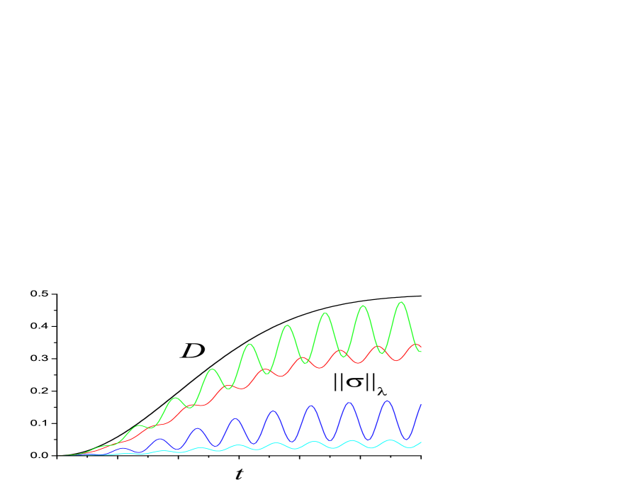
Figure 1: The maximal deviation norm $D$ vs. time for the spin-boson model with Ohmic bath. The non-monotonic curves illustrate the behaviour of the norm $\left\|\sigma(t)\right\|_{\lambda}$ for several initial choices of density operator $\rho(0)$.

Let us now consider the diamond norm $K(t)$ for one qubit. We will later use the result to estimate the norm $D(t)$ for the multi-qubit case. To find $K(t)$ for a two-level system one has to deal with the $4\times 4$ density matrix $\varrho_{jk,lm}$, where $j,k,l,m=1,2$. To evaluate

$$\varSigma\equiv\{\left(T-T^{(i)}\right){\raise 2.0pt\hbox{$\scriptscriptstyle{\otimes}$}}I\}\varrho,$$ (77)

one assumes that $T-T^{(i)}$ acts in the subspace labeled by the indices $j,l$, see (73,74), while the subspace labeled by the remaining pair of indexes, $k,m$, is unaffected. The resulting expression are

$$\varSigma_{2k,2m}=\frac{1}{2}\left[1-e^{-B^{2}(t)}\right]\left[\varrho_{1k,1m}-\varrho_{2k,2m}\right],$$ (78)

$$\varSigma_{2k,1m}=\frac{1}{2}\left[1-e^{-B^{2}(t)}\right]\left[\varrho_{1k,2m}-e^{-i\Omega t}\varrho_{2k,1m}\right],$$

$$\varSigma_{1k,1m}=-\varSigma_{2k,2m},\quad\varSigma_{1k,2m}=\varSigma_{2m,1k}^{*},\quad k,m=1,2.$$

The maximal trace norm of the $4\times 4$ matrix $\varSigma$ is calculated by considering the pure-state density matrices $\varrho=|\phi\rangle\langle\phi|$, similarly to the consideration in Section III, see (23-29). Here $|\phi\rangle$ can be expressed in terms of the basis states,

$$|\phi\rangle=\sum_{m,n=1,2}(a_{nm}+ib_{nm})|nm\rangle.$$ (79)

The constants $a_{nm}$, $b_{nm}$ are normalized real amplitudes, such that $\sum_{m,n=1,2}(a_{nm}^{2}+b_{nm}^{2})=1$. The eigenvalues of $\varSigma$, see (78), are $\varsigma_{1,2}=0$ and

$$\varsigma_{3,4}=\pm\left[\frac{1-e^{-B^{2}(t)}}{2}\right]\left\{1-4\left[(a_{11}a_{21}+a_{12}a_{22}+b_{11}b_{21}+b_{12}b_{22})\cos\left(\frac{\Omega t}{2}\right)\right.\right.$$

$$-\left.\left.(a_{21}b_{11}+a_{22}b_{12}-a_{11}b_{21}-a_{12}b_{22})\sin\left(\frac{\Omega t}{2}\right)\right]^{2}\right\}^{1/2}.$$ (80)

The maximal value corresponds to the square root in the expression (VI) equal to 1, and thus the diamond norm is

$$K(t)=1-e^{-B^{2}(t)}.$$ (81)

The above calculation establishes that $K(t)=2D(t)$ for the spin-boson model at short times, and (53) gives the upper bound on the multiqubit norm $D$,

$$D\lesssim\sum_{q}D_{q}=\frac{1}{2}\sum_{q}\left[1-e^{-B_{q}^{2}(t)}\right].$$ (82)

For short times, one can also establish a lower bound on $D(t)$. Consider a specific initial state with all the $Q$ qubits excited, $\rho(0)=(|2\rangle\langle 2|)_{1}{\raise 2.0pt\hbox{$\scriptscriptstyle{\otimes}$}}\ldots{\raise 2.0pt\hbox{$\scriptscriptstyle{\otimes}$}}(|2\rangle\langle 2|)_{Q}$. Then according to (71,72), $\rho(t)=\rho_{1}(t){{\raise 2.0pt\hbox{$\scriptscriptstyle{\otimes}$}}}\ldots{\raise 2.0pt\hbox{$\scriptscriptstyle{\otimes}$}}\rho_{Q}(t)$, where

$$\rho_{q}(t)=\frac{1}{2}\left\{\left[1-e^{-B^{2}_{q}(t)}\right]|1\rangle\langle 1|+\left[1+e^{-B^{2}_{q}(t)}\right]|2\rangle\langle 2|\right\}.$$ (83)

The right-bottom matrix element of the (diagonal) deviation operator,

$$\sigma_{2^{Q},2^{Q}}(t)=-1+2^{-Q}{\prod_{q}}\left[1+e^{-B^{2}_{q}(t)}\right],$$ (84)

can be expanded, for small times, as

$$\frac{1}{2}\sum_{q}B_{q}^{2}(t)+o\left(\sum_{q}B_{q}^{2}(t)\right),$$ (85)

because $B(t)$ vanishes for $t\to 0$. The largest eigenvalue of $\sigma(t)$ cannot be smaller than $\sigma_{2^{Q},2^{Q}}(t)$. It follows that

$$D\geq\frac{1}{2}\sum_{q}B^{2}_{q}+o\left(\sum_{q}B_{q}^{2}\right)=\sum_{q}D_{q}+o\left(\sum_{q}D_{q}\right),$$ (86)

where we used (76) for short times.

By combining the upper and lower bounds, we get the final result for short times,

$$D(t)=\sum_{q}D_{q}(t)+o\left(\sum_{q}D_{q}(q)\right).$$ (87)

VII Spin Model for Pure Decoherence

Let us consider a two-level system interacting with the bosonic bath of the environmental modes adiabatically, i.e., without exchange of energy with the bath modes basis . While energy exchange processes are needed for thermalization, and also contribute to decoherence, additional, “pure” decoherence processes are possible and are expected to be important at low temperatures and short to intermediate times, appropriate for quantum computing designs short . The spin-model Hamiltonians $H_{S}$ and $H_{B}$ will still be assumed of the form

$$H_{S}={-\frac{\Omega}{2}}\sigma_{z},$$ (88)

$$H_{B}=\sum\limits_{k}\omega_{k}a_{k}^{\dagger}a_{k}.$$ (89)

However, the interaction term will be now of the form commuting with the system’s energy, thus making the latter conserved,

$$H_{I}=\sigma_{z}\sum_{k}{\left(g_{k}^{\vphantom{\dagger}}a_{k}^{\dagger}+g_{k}^{*\vphantom{\dagger}}a_{k}^{\vphantom{\dagger}}\right)}.$$ (90)

Since $H_{S}$ commutes with $H_{I}$, instead of the approximate formula (59) we have the exact factorization,

$$e^{i(H_{S}+H_{B}+H_{I})t}=e^{iH_{S}t/2}\,e^{i(H_{B}+H_{I})t}\,e^{iH_{S}t/2}.$$ (91)

Therefore, the analytical expression for the reduced density operator (61) is exact and valid for all times vanKampen ; basis . For the two-level case Palma ,

$$\rho_{11}(t)=\rho_{11}(0),$$ (92)

$$\rho_{22}(t)=\rho_{22}(0),$$ (93)

$$\rho_{12}(t)=\rho_{12}(0)e^{i\Omega t-B^{2}(t)},$$ (94)

where the spectral function $B(t)$ was defined in (62). The diagonal density matrix elements remain constant because there is no energy exchange of the system with the bath. However, there is pure (adiabatic) decoherence manifested by the decay of the off-diagonal elements, characterized by the spectral function $B(t)$ (94). The corresponding deviation matrix is expressed as follows,

$$\sigma_{11}(t)=\sigma_{22}(t)=0,$$ (95)

$$\sigma_{12}=\rho_{12}(0)e^{i\Omega t-B^{2}(t)}.$$ (96)

The operator norm of $\sigma$ is

$$\left\|\sigma(t)\right\|_{\lambda}=\left[1-e^{-B^{2}(t)}\right]\left|\rho_{12}\right|.$$ (97)

Since both diagonal elements of the density matrix and its eigenvalues are in $[0,1]$ it follows that the absolute value of the off-diagonal element of any two-level-system density matrix less than $1/2$,

$$\left|\rho_{12}\right|\leq\frac{1}{2}.$$ (98)

Thus,

$$D(t)=\sup_{\rho(0)}\big{(}\|\sigma(t,\rho(0))\|_{\lambda}\big{)}=\frac{1}{2}\left[1-e^{-B^{2}(t)}\right].$$ (99)

One can also evaluate

$$\varSigma=\{\left(T-T^{(i)}\right){\raise 2.0pt\hbox{$\scriptscriptstyle{\otimes}$}}I\}\varrho,$$ (100)

$$\varSigma_{jk,jm}=0,$$ (101)

$$\varSigma_{1k,2m}=\varSigma_{2m,1k}^{*}=\varrho_{1k,2m}(0)e^{i\Omega t-B^{2}(t)}$$ (102)

For $\varrho=|\phi\rangle\langle\phi|$, with $|\phi\rangle$ as in (79), the eigenvalues of $\varSigma$ are $\varsigma_{1}=\varsigma_{2}=0$ and

$$\varsigma_{3,4}=\pm\left[1-e^{-B^{2}(t)}\right]\sqrt{\left(\varrho_{11,11}+\varrho_{12,12}\right)\left(\varrho_{21,21}+\varrho_{22,22}\right)}.$$ (103)

Since

$$\rm{Tr}\varrho=1,$$ (104)

one can show that

$$\lambda_{3,4}=\pm\left[1-e^{-B^{2}(t)}\right]\sqrt{x(1-x)},$$ (105)

with

$$x=\varrho_{11,11}+\varrho_{12,12}$$ (106)

satisfying $0\leq x\leq 1$. The diamond norm (37) thus follows,

$$K(t)=\underset{{0\leq x\leq 1}}{\sup}\left\{2\left[1-e^{-B^{2}(t)}\right]\sqrt{x(1-x)}\right\}=1-e^{-B^{2}(t)}.$$ (107)

It is instructive to compare (99,107) and (76,81). The results are identical despite the fact that the interaction terms and density matrix time-dependence (71,72,92,94) are different. As in the case of the short-time approximation, we get the upper bound for the multiqubit norm $D(t)$, (53).

To establish the lower bound on $D(t)$, we consider a specific initial state with $\rho(0)=|\Psi\rangle\langle\Psi|$, which is a superposition of the state corresponding to all the qubits in their ground states and that of all qubits in their excited states,

$$|\Psi\rangle=\frac{1}{\sqrt{2}}\left(|1\ldots 1\rangle+|2\ldots 2\rangle\right).$$ (108)

Then according to (92,94),

$$\rho_{1,1}(t)=\rho_{2^{Q},2^{Q}}(t)=\frac{1}{2},$$ (109)

$$\rho_{1,2^{Q}}(t)=\frac{1}{2}\exp{\Big{[}-i\sum_{q}\Omega_{q}t-\sum_{q}B^{2}_{q}(t)\Big{]}}.$$ (110)

The only non-zero matrix elements of the deviation operator are the right-top and left-bottom matrix elements,

$$\sigma_{1,2^{Q}}(t)=-\frac{1}{2}\left[1-e^{-\sum_{q}B^{2}_{q}(t)}\right]e^{it\sum_{q}\Omega_{q}},$$ (111)

For short times, the absolute value of $\sigma_{1,2^{Q}}(t)$ can be expressed as

$$\frac{1}{2}\sum_{q}B_{q}^{2}(t)+o\left(\sum_{q}B_{q}^{2}(t)\right),$$ (112)

where the first term gives the largest eigenvalue of $\sigma(t)$. It follows that

$$D\geq\frac{1}{2}\sum_{q}B^{2}_{q}+o\left(\sum_{q}B_{q}^{2}\right)=\sum_{q}D_{q}+o\left(\sum_{q}D_{q}\right),$$ (113)

where we used (99) for short times. Finally, we get the same result (87) for the approximate additivity of $D$ for short times, for the present model of adiabatic decoherence,

$$D(t)=\sum_{q}D_{q}(t)+o\left(\sum_{q}D_{q}(t)\right).$$ (114)

In summary, we introduced the maximal operator norm suitable for evaluation of decoherence for quantum system immersed in a noisy environment. The new maximal operator norm was evaluated for spin models with two types of bosonic bath interaction. We established both general and model specific subadditivity and additivity properties of this measure of decoherence for multi-qubit system at short times. The latter property allows evaluation of decoherence for complex systems in the regime of interest for quantum computing applications.

This research was supported by the National Security Agency and Advanced Research and Development Activity under Army Research Office contract DAAD-19-02-1-0035, and by the National Science Foundation, grant DMR-0121146.

References

- (1) G. W. Ford, M. Kac and P. Mazur, J. Math. Phys. 6, 504 (1965).
- (2) A. O. Caldeira and A. J. Leggett, Physica A 121, 587 (1983).
- (3) S. Chakravarty and A. J. Leggett, Phys. Rev. Lett. 52, 5 (1984).
- (4) H. Grabert, P. Schramm and G.-L. Ingold, Phys. Rep. 168, 115 (1988).
- (5) N. G. van Kampen, J. Stat. Phys. 78, 299 (1995).
- (6) K. M. Fonseca Romero and M. C. Nemes, Phys. Lett. A 235, 432 (1997).
- (7) C. Anastopoulos and B. L. Hu, Phys. Rev. A 62, 033821 (2000).
- (8) G. W. Ford and R. F. O’Connell, Phys. Rev. D 64, 105020 (2001).
- (9) D. Braun, F. Haake and W. T. Strunz, Phys. Rev. Lett. 86, 2913 (2001).
- (10) G. W. Ford, J. T. Lewis and R. F. O’Connell, Phys. Rev. A 64, 032101 (2001).
- (11) J. Wang, H. E. Ruda and B. Qiao, Phys. Lett. A 294, 6 (2002).
- (12) E. Lutz, Phys. Rev. A 67, 022109 (2003); cond-mat/0208503 (2002).
- (13) A. Khaetskii, D. Loss and L. Glazman, Phys. Rev. B 67, 195329 (2003).
- (14) R. F. O’Connell and J. Zuo, Phys. Rev. A 67, 062107 (2003).
- (15) W. T. Strunz, F. Haake and D. Braun, Phys. Rev. A 67, 022101 (2003).
- (16) W. T. Strunz and F. Haake, Phys. Rev. A 67, 022102 (2003).
- (17) V. Privman, D. Mozyrsky and I. D. Vagner, Comp. Phys. Commun. 146, 331 (2002).
- (18) V. Privman, J. Stat. Phys. 110, 957 (2003).
- (19) V. Privman, Mod. Phys. Lett. B 16, 459 (2002).
- (20) P. W. Shor, Phys. Rev. A 52, R2493 (1995).
- (21) A. M. Steane, Phys. Rev. Lett. 77, 793 (1996).
- (22) C. H. Bennett, G. Brassard, S. Popescu, B. Schumacher, J. A. Smolin and W. K. Wootters, Phys. Rev. Lett. 76, 722 (1996).
- (23) A. R. Calderbank and P. W. Shor, Phys. Rev. A 54, 1098 (1996).
- (24) A. M. Steane, Phys. Rev. A 54, 4741 (1996).
- (25) D. Aharonov and M. Ben-Or, quant-ph/9611025 (1996).
- (26) D. Gottesman, Phys. Rev. A 54, 1862 (1997).
- (27) E. Knill and R. Laflamme, Phys. Rev. A 55, 900 (1997).
- (28) D. Loss and D. P. DiVincenzo, cond-mat/0304118 (2003).
- (29) V. Privman, Proc. SPIE 5115, 345 (2003).
- (30) W. H. Zurek, Rev. Mod. Phys. 75, 715 (2003).
- (31) A. Shnirman and G. Schön, cond-mat/0210023 (2002).
- (32) L. Fedichkin, A. Fedorov and V. Privman, Proc. SPIE 5105, 243 (2003).
- (33) L. Fedichkin and A. Fedorov, quant-ph/0309024 (2003).
- (34) L. Fedichkin, A. Fedorov and V. Privman, cond-mat/0309685 (2003).
- (35) A. O. Caldeira and A. J. Leggett, Phys. Rev. Lett. 46, 211 (1981).
- (36) S. Lloyd, Phys. Rev. Lett. 75, 346 (1995).
- (37) A. Barenco, C. H. Bennett, R. Cleve, D. P. DiVincenzo, N. Margolus, P. Shor, T. Sleator, J. A. Smolin and H. Weinfurter, Phys. Rev. A 52, 3457 (1995).
- (38) S. Lloyd, Science 261, 1569 (1993).
- (39) Q. A. Turchette, C. J. Hood, W. Lange, H. Mabuchi, and H. J. Kimble, Phys. Rev. Lett. 75, 4710 (1995).
- (40) J. I. Cirac and P. Zoller, Phys. Rev. Lett. 74, 4091 (1995).
- (41) A. Ekert and R. Jozsa, Rev. Mod. Phys. 68, 733 (1996).
- (42) V. Privman, I. D. Vagner and G. Kventsel, Phys. Lett. A239, 141 (1998).
- (43) B. E. Kane, Nature 393, 133 (1998).
- (44) D. Loss and D. P. DiVincenzo, Phys. Rev. A 57, 120 (1998).
- (45) A. Imamoglu, D. D. Awschalom, G. Burkard, D. P. DiVincenzo, D. Loss, M. Sherwin and A. Small, Phys. Rev. Lett. 83, 4204 (1999).
- (46) P. Zanardi and F. Rossi, Phys. Rev. B 59, 8170 (1999).
- (47) Y. Nakamura, Yu. A. Pashkin, and H. S. Tsai, Nature 398, 786 (1999).
- (48) T. Tanamoto, Phys. Rev. A 61, 022305 (2000).
- (49) P. M. Platzman and M. I. Dykman, Science 284, 1967 (1999).
- (50) G. P. Sanders, K. W. Kim, W. C. Holton, Phys. Rev. A 60, 4146 (1999); quant-ph/9909070 (1999).
- (51) G. Burkard, D. Loss, D. P. DiVincenzo, Phys. Rev. B 59, 2070 (1999).
- (52) R. Vrijen, E. Yablonovitch, K. Wang, H. W. Jiang, A. Balandin, V. Roychowdhury, T. Mor and D. P. DiVincenzo, Phys. Rev. A 62, 012306 (2000).
- (53) L. Fedichkin, M. Yanchenko and K. A. Valiev, Nanotechnology 11, 387 (2000).
- (54) S. Bandyopadhyay, Phys. Rev. B 61, 13813 (2000).
- (55) A. A. Larionov, L. E. Fedichkin, and K. A. Valiev, Nanotechnology 12, 536 (2001).
- (56) N. G. van Kampen, Stochastic Processes in Physics and Chemistry, North-Holland, 2001.
- (57) W. H. Louisell, Quantum Statistical Properties of Radiation, Wiley, 1973.
- (58) A. Abragam, The Principles of Nuclear Magnetism, Clarendon Press, 1983.
- (59) K. Blum, Density Matrix Theory and Applications, Plenum, 1996.
- (60) A. Y. Kitaev, Russ. Math. Surv. 52, 1191 (1997).
- (61) D. Aharonov, A. Kitaev and N. Nisan, Proc. XXXth ACM Symp. Theor. Comp., Dallas, TX, USA, 20 (1998).
- (62) A. Yu. Kitaev, A. H. Shen and M. N. Vyalyi, Classical and Quantum Computation, AMS, 2002.
- (63) J. Preskill, Proc. Roy. Soc. Lond. A 454, 385 (1998).
- (64) D. P. DiVincenzo, Fort. Phys. 48, 771 (2000).
- (65) M. J. Storcz and F. K. Wilhelm, Phys. Rev. A 67, 042319 (2003).
- (66) G. M. Palma, K. A. Suominen and A. K. Ekert, Proc. Roy. Soc. Lond. A 452, 567 (1996).
- (67) L.-M. Duan and G.-C. Guo, Phys. Rev. Lett. 79, 1953 (1997).
- (68) P. Zanardi and M. Rasetti, Phys. Rev. Lett. 79, 3306 (1997).
- (69) D. A. Lidar, I. L. Chuang and K. B. Whaley, Phys. Rev. Lett. 81, 2594 (1998).
- (70) B. J. Dalton, J. Mod. Opt. 50, 951 (2003).
- (71) V. Privman, D. Mozyrsky and I. D. Vagner, Comp. Phys. Commun. 146, 331 (2002).
- (72) J. von Neumann, Mathematical Foundations of Quantum Mechanics, Princeton University Press, 1983.
- (73) J. I. Kim, M. C. Nemes, A. F. R. de Toledo Piza and H. E. Borges, Phys. Rev. Lett. 77, 207 (1996).
- (74) W. H. Zurek, S. Habib and J. P. Paz, Phys. Rev. Lett. 70, 1187 (1993).
- (75) J. C. Retamal and N. Zagury, Phys. Rev. A 63, 032106 (2001).
- (76) L.-M. Duan and G.-C. Guo, Phys. Rev. A 56, 4466 (1997).
- (77) T. Kato, Perturbation Theory for Linear Operators, Springer-Verlag, 1995.
- (78) A. J. Leggett, S. Chakravarty, A. T. Dorsey, M. P. A. Fisher, A. Garg and W. Zwerger, Rev. Mod. Phys. 59, 1 (1987).
- (79) D. Mozyrsky and V. Privman, J. Stat. Phys. 91, 787 (1998).