The spin resonance and high frequency optical properties of the cuprates.

Abstract

We argue that recently observed superconductivity-induced blue shift of the plasma frequency $\delta\omega_{pl}$ in $Bi_{2}Sr_{2}CaCu_{2}O_{8+\delta}$ vdm is related to the change in the integrated dynamical structure factor associated with the development of the spin resonance below $T_{c}$. We show that the magnitude of $\delta\omega_{pl}$ is consistent with the small integrated spectral weight of the resonance, and its temperature dependences closely follow that of the spin resonance peak.

The importance of the resonance spin mode for the physics of the cuprates continue to be the subject of intensive debate. In a generic superconductor, the pairing of fermions drastically reduces the damping of collective spin degrees of freedom at energies below $2\Delta$. For a $d-$wave superconductor, the residual interaction between spin fluctuations and fermions gives rise to the additional effect – the development of the exciton mode below $2\Delta$ (see e.g. Ref. mike_1 and references therein). This mode exists for bosonic momenta near $(\pi,\pi)$ and is commonly called the “spin resonance”. It has been observed in three different families of high-$T_{c}$ superconductors  rosa ; fong ; dai ; bi ; keimer . This mode is not a “glue” to superconductivity as it emerges only in the superconducting state (more precisely, below the pseudogap temperature), but it affects electronic properties of the cuprates in the superconducting state.

Much of recent works on the effect of the spin resonance on electrons was concentrated on whether the interaction with the resonance is capable to explain experimentally detected low-energy features in the fermionic spectral function, tunneling density of states and optical conductivity mike_1 ; acs . An example of this behavior is the peak/dip/hump structure of the spectral function ARPES_pdh .

The spin-resonance scenario for the cuprates was recently questioned kee on the basis that the measured spectral weigh of the resonance is only $1-2$ percent of the total magnetic spectral weight. Ar. Abanov et al., however, argued  reply that this smallness merely reflects the fact that the resonance exists only in a narrow momentum range near ${\bf Q}=(\pi/a,\pi/a)$ [roughly, between ${\bf Q}$ and $0.8{\bf Q}$], while at momenta where the resonance does exist, it strongly couples to fermions. They further argued that at small $\omega\sim 2\Delta$, the fermionic self-energy change between normal and superconducting states chiefly comes from spin fluctuations with energies comparable to $\omega$, and from spin momenta $|{\bf q}-{\bf Q}|\sim\omega/v_{F}$, where $v_{F}$ is the bare Fermi velocity. As $v_{F}\sim 1eV*a$ is large, typical spin momenta for $\omega\leq 100meV$ are well within the range where the resonance does exist, i.e., the smallness of the total spectral weight of the resonance does not matter.

The subject of the present communication is the analysis of the possible role of the spin resonance in the observed changes between normal and superconducting state in the optical data at high frequencies, $\omega\sim 0.5-1eV$. Recently, Molegraaf et al. reported the results of their ellipsometry measurements on optimally doped and underdoped $Bi_{2}Sr_{2}CaCu_{2}O_{8+\delta}$ with $T_{c}=88K$ and $T_{c}=66K$ respectively vdm . They observed that in the normal state, the in-plane plasma frequency increases as $T^{2}$ with decreasing $T$, however below $T_{c}$ it increases faster such that the actual value of $\omega_{pl}(T=0)$ is larger than the extrapolation from the normal state. The effect is very small: at optimal doping $\delta\omega_{pl}\sim 10cm^{-1}$ is only $1.3\times 10^{-3}$ of the plasma frequency $\omega_{pl}\sim 7600cm^{-1}\approx 1eV$, but detectable by the ellipsometry technique.

The change of the plasma frequency in a superconductor is related to the change of the fermionic self-energy between superconducting and normal states (see Eq. (3) below). Conventional wisdom holds that at $\omega\sim\omega_{pl}$, which well exceed the magnetic bandwidth, interaction with low-energy spin fluctuations is not the dominant mechanism for the fermionic self-energy. We argue, however, that while this is generally true for $\Sigma(\omega)$ itself, $\delta\omega_{pl}$ scales with $\delta\Sigma(\omega)=\Sigma_{sc}(\omega)-\Sigma_{n}(\omega)$, and the latter comes from frequencies comparable to the superconducting gap and can be captured within the low-energy, spin-fluctuation theory. We will see, however, that at high $\omega$, the concept that intermediate fermions and bosons have equal energies fails, and a fermion with energy $1eV$ interacts with the whole band of magnetic fluctuations. As a result, $\delta\Sigma(\omega)$ scales with the integrated magnetic spectral weight, and the smallness of the spectral weight transfer into the resonance becomes crucial. We argue that the value of the observed shift of the plasma frequency is consistent with the fact that only $1-2\%$ of the magnetic spectral weight is transferred into the resonance.

Our reasoning is the following. At plasma frequency, the real part of the dielectric function $\epsilon(\omega)$ changes sign. The dielectric function obeys $\epsilon(\omega)=\epsilon(\infty)+4\pi i\sigma(\omega)/\omega$, where $\sigma(\omega)$ is the optical conductivity. By Kubo formula, $\sigma(\omega)=((\omega^{0}_{pl})^{2}/(4\pi))Re[\Pi(\omega)/(-i\omega)]$ where $\Pi(\omega)$ is fully renormalized current-current polarization operator and $(\omega^{0}_{pl})^{2}=4\pi ne^{2}/m$ is the bare plasma frequency. The plasma frequency is then the solution of

$$\omega_{pl}=\frac{\omega^{0}_{pl}}{\sqrt{\epsilon(\infty)}}~{}\sqrt{Re\Pi(\omega_{pl})}$$ (1)

To zero-order approximation, $\Pi(\omega_{pl})=1$, i.e., $\omega_{pl}=\omega^{0}_{pl}/\sqrt{\epsilon(\infty)}$. However, at any finite frequency $1-Re\Pi(\omega)$ is still finite, and hence $\omega_{pl}$ is sensitive to the change of the polarization operator upon entering the superconducting state. This change of $\omega_{pl}$ is small as superconductivity mostly affects the form of $\Pi(\omega)$ at frequencies comparable to the superconducting gap $\Delta\sim 0.04\omega_{pl}$.

At high frequencies, $\omega\sim 1eV$, normal and anomalous fermionic self-energies $\Sigma({\bf k},\omega)\approx\Sigma(\omega)$ and $\Phi({\bf k},\omega)$ are both small compared to $\omega$, and to the leading order in the self-energy, the current-current correlator both in the normal and superconducting states is given by

$$\Pi(\Omega)=\int_{0}^{\Omega}\frac{d\omega}{\Omega+\Sigma(\omega)+\Sigma(\Omega-\omega)}$$ (2)

Substituting this expression into (1) we find that the superconductivity-induced change in the plasma frequency at $T=0$ is related to the difference between superconducting and normal fermionic self-energies $\delta\Sigma(\omega)=\Sigma^{sc}(\omega)-\Sigma^{n}(\omega)$ as

$$\frac{\delta\omega_{pl}}{\omega_{pl}}=-\frac{1}{2\Pi^{\prime}_{n}(\omega_{pl})}~{}$$

$$\!\!\!\!\!\times Re \!\!\!\!\!\int_{0}^{\omega_{pl}}\!\!\!\!\!d\omega~{}\frac{\delta\Sigma(\omega)+\delta\Sigma(\omega_{pl}-\omega)}{\left[\omega_{pl}+\omega Z_{\omega}+(\omega_{pl}-\omega)Z_{\omega_{pl}-\omega}\right]^{2}}$$ (3)

where $\delta\omega_{pl}=\omega^{sc}_{pl}-\omega^{n}_{pl}$, $\Pi^{\prime}_{n}(\omega)$ is the real part of the polarization operator in the normal state, and $Z_{\omega}=1+\Sigma_{n}(\omega)/\omega$ is inverse quasiparticle residue in the normal state. By all accounts, at $\omega\sim\omega_{pl}$, $\Sigma(\omega)\ll\omega$, i.e., $Z_{\omega}\approx 1$. Hence, once the integral in (3) is dominated by frequencies where either $\omega$ or $\omega_{pl}-\omega$ are near $\omega_{pl}$ (as we later verify), the precise form of the fermionic $Z(\omega)$ at high frequencies does not matter, and $\delta\omega_{pl}/\omega_{pl}\approx\delta\Sigma(\omega_{pl})/(2\omega_{pl})$.

The computation of $\delta\omega_{pl}$ therefore reduces to the computation of the self-energy difference between normal and superconducting states. We present the result for $\delta\Sigma(\omega)$ now and discuss its derivation later. We found that, within the spin-fluctuation scenario, there are two distinct frequency regimes depending, roughly, on whether or not $\omega$ exceeds the magnetic bandwidth. At small frequencies, the Eliashberg approximation is valid, and $\delta\Sigma(\omega)$ is positive (see Fig. 3). In this regime, internal fermions and bosons in the self-energy diagram have comparable energies, i.e., a fermion is interacting only with spin fluctuations very near ${\bf Q}$. We verified that if this behavior extended up to $\omega\sim\omega_{pl}$, $\delta\omega_{pl}$ would be negative, in disagreement with the data.

At larger frequencies, however, Eliashberg approximation becomes invalid, and a novel (anti-Eliashberg) approximation has to be used. In this approximation, we obtained that the change of the fermionic self-energy is proportional to the integrated change of the dynamical spin structure factor

$$\delta\Sigma(\omega)\approx-\frac{3g^{2}}{Z_{\omega}\omega}\int\frac{d\Omega d^{2}q}{8\pi^{3}}\sum_{i}\delta S_{i}({\bf q},\Omega)F({\bf q})$$ (4)

where $g$ is the spin-fermion coupling constant estimated to be $g\sim 0.7eV$ acs ; mike_1 ; reply , and $\delta S_{i}({\bf q},\Omega)=S^{sc}_{i}({\bf q},\Omega)-S^{n}_{i}({\bf q},\Omega)$ is the change in the dynamical structure factor $S({\bf q},\Omega)=\chi^{\prime\prime}({\bf q},\Omega)(1+\coth(\omega/2T))$ in even ($i=1$) and odd ($i=2$) channels. The factor $F({\bf q})$ decreases away from ${\bf Q}$ but can be safely approximated by $F({\bf q})=1$ in the narrow momentum range where the resonance is experimentally detectable. The integrated magnetic spectral weight near $(\pi,\pi)$ is larger in the superconducting state fong ; dai , hence at high frequencies $\Sigma^{\prime}(\omega)$ is smaller in a superconductor. Using this $\delta\Sigma(\omega)$ we find that $\delta\omega_{pl}$ is positive, in agreement with vdm .

The crossover between the two regimes occurs at optimal doping at $\omega=\omega_{0}\sim 300meV$, see Fig. 2. Theoretically, we use one-band model to get Eq. 4, i.e., we assume that there is a frequency range above $\omega_{0}$, where anti-Eliashberg approximation is valid, but interband transitions still can be neglected. The applicability of this approximation has to be verified by comparing the results of one-band analysis with the data.

The momentum and frequency integral in the r.h.s. of (4) yields $BS(S+1)/3$ where $B$ is the percentage of the spectral weight redistributed below $T_{c}$. Only the odd channel contributes to $\delta S({\bf q},\Omega)$ and $1-2\%$ of the spectral weight from this channel is redistributed fong , i.e., $B\sim 0.005-0.01$. Substituting $\delta\Sigma(\omega)\approx-3g^{2}B/(4\omega)$ into the expression for $\delta\omega_{pl}$ we obtain $\delta\omega_{pl}/\omega_{pl}\sim(1-2)\times 10^{-3}$, in near perfect agreement with the experimental result $1.3\times 10^{-3}$ vdm . We emphasize that the agreement is entirely due to the fact that the integrated weight of the resonance is very small. If it wasn’t, the blue shift of the plasma frequency would be much larger. To verify the prefactor, we went beyond estimates and evaluated the full integral in (3) using the normal state expression for $Z_{\omega}$ acs : $Z_{\omega}\approx 1+(i{\bar{\omega}}/\omega)^{1/2}$ where ${\bar{\omega}}\sim 0.35g$. We obtained almost the same result for $\delta\omega_{pl}$ as above – the extra prefactor is $0.97\approx 1$.

In Fig.1 we plot the temperature dependence of $\delta\omega_{pl}(T)$ together with the temperature dependence of the resonance peak intensity dai . The data for the fully integrated intensity are available for fewer temperatures and show roughly the same $T$ dependence dai . We see that the $T$ dependences of $\delta\omega_{pl}$ and of the resonance peak follow each other as it should be according to Eq. (4).

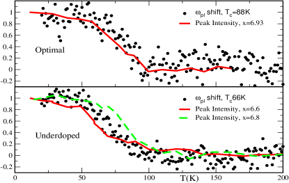
Figure 1: The temperature dependence of the superconductivity-induced change of the plasma frequency in $Bi2212$ vdm vs the change in the resonance peak intensity for $YBCO$ dai . Upper panel - optimal doping, lower panel - underdoped samples. We plot $YBCO$ data for two different underdoped samples for comparison.

We also searched for the explanation of the $T^{2}$ temperature dependences of $\omega_{pl}$ found by Molegraaf et al. in the normal state. The analysis of the neutron data fong shows that the dominant source of the temperature dependence of the spectral function is the $T$ dependence of $\chi^{\prime\prime}(\omega)$, while the one from $(1+\coth\omega/(2T))$ is much weaker. Indeed, the neutron data presented for $\omega=65meV$ fong show that the local $\chi^{\prime\prime}(\omega)$ decreases by more than the factor of $2$ between $100$ and $200K$, when the thermal factor $\coth(\omega/2T)\approx 1$ for both temperatures. It is therefore likely that the $T$ dependence in the normal state originates in thermal corrections to the parameters of the dynamical spin susceptibility (i.e., to the magnetic correlation length). Theoretically, these corrections form regular series in $(T/E_{F})^{2}$ acs , hence the temperature dependence of $\omega_{pl}$ must be $T^{2}$, unless superconductivity interferes.

We now turn to the conductivity. Molegraaf et al. reported that the Drude optical spectral weight integrated up to a frequency of $10000cm^{-1}$ (including the condensate contribution) increases below $T_{c}$, and argued that this increase is compensated by the decrease of the optical spectral weight integrated between $10000cm^{-1}$ and $20000cm^{-1}$, where interband transitions are overly relevant. This, they argued, implies that the condensate contribution to $\sigma_{1}(\omega)$ is not compensated by the reduction of the conductivity in the superconducting state up to frequencies when one-band description fails.

Our results are inconsistent with this claim. The optical integral $\delta I(\Omega)=\hbar^{2}\int^{\Omega}_{0}\delta\sigma(\omega)d\omega$ for $\Omega\sim 1eV$ covers the range of frequencies where the Eliashberg approximation is valid ($\delta I_{1}$) , and the range where Eq. (4) is valid ($\delta I_{2}$). Using Eq. (4), we can compute the partial integral $\delta I_{2}(\Omega)=\hbar^{2}\int^{\Omega}_{\omega_{0}}\delta\sigma(\omega)d\omega$ where, we remind, $\omega_{0}$ is the lower boundary for the applicability of Eq. (4). The approximations for $\sigma$ are less robust than for $\omega_{pl}$ as for the conductivity we need to know $ImZ_{\omega}$ at high frequencies, where the use of the low-energy theory is questionable. Still, at high frequencies, $Im[1/Z(\omega)]\approx-Im\Sigma(\omega)/\omega$ is negative, hence, according to (4), the high-frequency conductivity $\sigma(\omega)\sim 1/\omega^{2}\tau(\omega)\propto\Sigma^{\prime\prime}(\omega)$ is larger in the superconducting state than in the normal state extrapolated to $T=0$. Accordingly, $\delta I_{2}(\Omega)$ is positive. Substituting Eqs. (2) and (4) into the Kubo formula, and evaluating the integrals with the same $Z(\omega)$ as above, we obtain $\delta I_{2}(\Omega)\approx(2-4)\times 10^{-3}(eV)^{2}$ for $\Omega\sim 1eV$.

The integral for $\delta I_{2}(\Omega)$ converges at the upper limit; formally taking $\Omega=\infty$ yields almost the same $\delta I_{2}$. As the $f-$sum rule must be satisfied within the one-band model (if the bandwidth is formally set to infinity), the value $-\delta I_{2}(\infty)$ gives the estimate of the optical integral $\delta I_{1}(\omega_{0})$ over frequencies where the Eliashberg theory is valid. From our consideration, this integral is negative, i.e., the condensate contribution is overcompensated by the reduction of the conductivity in the superconducting state below $\omega_{0}$ comm3 . As an independent check, we computed optical integral $\delta I_{1}$ within Eliashberg theory ac_2 , and indeed obtained that $\delta I_{1}$ changes sign at $\omega\sim 300meV$ at optimal doping (see Fig.3). The accuracy of our Eliashberg calculations is not sufficient to compare the values of the two contributions to $\delta I$.

Our results therefore indicate that at $T=0$, the full optical integral is exchausted at frequencies smaller than the bandwidth. The optical integral evaluated over larger frequencies is larger at $T=0$ than in the normal state extrapolated to $T=0$. The crossover frequency $\omega_{0}$ somewhat increases with underdoping (see caption for Fig.3) but theoretically it still remains $O({\bar{\omega}})$ even in strongly underdoped materials homes . Note that this does not contradict the idea that that superconductivity is driven by the decrease of the kinetic energy norman_pepin , as within the same approach, the decrease of the kinetic energy also comes from frequencies $(1-2){\bar{\omega}}$ rob .

We now describe the calculation of the self-energy, Eq. (4) in some detail. We assume that the fermionic self-energy predominantly comes from the fermion-fermion interaction in the spin channel and can be viewed as being mediated by spin collective modes with momenta near $(\pi,\pi)$. Quite generally, the imaginary part of the fermionic self-energy is given by

$$\Sigma^{\prime\prime}({\bf k},\omega) = \frac{3}{8\pi^{3}}\int{\tilde{g}}^{2}\chi^{\prime\prime}({\bf q},\Omega)~{}G^{\prime\prime}({\bf k}+{\bf q},\omega+\Omega)~{}$$ (5)

$$\left[\tanh{\frac{\omega-\Omega}{2T}}+\coth{\frac{\Omega}{2T}}\right]d\Omega d^{2}q$$

where ${\tilde{g}}$ is the fully renormalized vertex, $\chi({\bf q},\Omega)$ is the propagator of the collective mode, and $G({\bf k}+{\bf q},\omega+\Omega)$ is the full fermionic Green’s function.

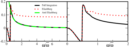
Figure 2: Right panel - the difference in the electronic self-energy between normal and superconducting states calculated explicitly and using Eliashberg and anti-Eliashberg approximations. The frequency is measured in units of ${\bar{\omega}}\sim 0.35g\sim 250meV$. Clearly, the anti-Eliashberg approximation is much better at large frequencies. Left panel - the low-frequency region, where the Eliashberg approximation is valid.

At small frequencies, the physics that allows one to neglect vertex corrections (i.e., set ${\tilde{g}}=g$), is the fact that at strong coupling, spin fluctuations are overdamped in the normal state and are slow modes compared to electrons. Hence, an effective Migdal theorem is valid acs . By the same reason, the momentum integration in Eqn (5) is factorized – the integration transverse to the Fermi surface involves only fast fermion, while the integration along the Fermi surface is over a slow bosonic momentum. This computational procedure is called Eliashberg approximation. It describes the jump in $\Sigma^{\prime\prime}$ at $\Delta+\omega_{res}$ that is the key element of the peak/dip/hump behavior mike_1 ; acs . However, for $\delta\Sigma(\omega)$ this approximation is valid only as long as external fermionic frequency $\omega$ is smaller than a typical frequency at which the momentum integral of $\delta\chi^{\prime\prime}(\Omega)$ converges. At strong coupling, this generally happens at $\Omega$ comparable to the effective bosonic bandwidth ${\bar{\omega}}$ defined such that in the normal state, $\Sigma(\omega)$ becomes less than $\omega$ at $\omega>{\bar{\omega}}$, i,e., spin-fluctuation scattering becomes ineffective. When spin-fermion coupling $g$ is less than the fermionic bandwidth $W$, ${\bar{\omega}}\sim 0.35{\bar{g}}$, in the opposite limit ${\bar{\omega}}\sim W^{2}/g\sim J$. Note that within the same model, $\Delta\sim 0.3{\bar{\omega}}$ acs .

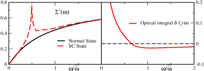
Figure 3: The results of Eliashberg calculations for coupling $\lambda=1$. Left panel - self-energy, right panel - the optical integral $\delta I(\omega)$ (including the condensate piece). For $\lambda=2$, $\delta I(\omega)$ changes sign at a larger $\omega\sim 2{\bar{\omega}}$.

When $\omega\gg{\bar{\omega}}$, and $k\approx k_{F}$, $G^{\prime\prime}({\bf k}+{\bf q},\omega+\Omega)\approx Im(\omega Z_{\omega})^{-1}$, and it can be taken out of the integral. To the same accuracy, the $T$ dependent factor in (5) is approximated by $1+\coth(\Omega/2T)$. We then obtain:

$$Im\left[\delta\Sigma(\omega)\right]=-3g^{2}~{}Im\left[\frac{1}{Z_{\omega}\omega}\right]~{}\times$$

$$\int\frac{d\Omega d^{2}q}{8\pi^{3}}\sum_{i}\delta S_{i}({\bf q},\Omega)F({\bf q})$$ (6)

where $F({\bf q})$ subject to $F({\bf Q})=1$ decreases at $|{\bf Q}-{\bf q}|=O(|{\bf Q}|)$ and reflects the fact that the spin-fermion model is only valid for bosonic momenta near $(\pi,\pi)$. As the Kramers-Kronig transform of (6) is infrared convergent, the full self-energy is given by (4).

We find therefore that at high frequencies $\omega\gg{\bar{\omega}}$, the correct computational procedure for $\delta\Sigma(\omega)$ is opposite to the Eliashberg approximation – instead of factorizing the momentum integral, one can neglect the momentum dependence in the Green’s function and perform the full 2D momentum integration over the bosonic momenta. We verified that in this, anti-Eliashberg approximation, vertex corrections are again small, this time in ${\bar{\omega}}/\omega$, such that ${\tilde{g}}=g$ in Eq. (5).

Obviously, there should be a crossover between Eliashberg and anti-Eliashberg approximations as frequency increases. To understand where it is located, we evaluated $\delta\Sigma^{\prime\prime}(\omega)$ explicitly, using the normal and superconducting forms of the dynamical spin susceptibility obtained earlier acs , and compared the full result with the two approximate forms. The results are presented in Fig. 2. We see that for $\omega\leq{\bar{\omega}}$, Eliashberg approximation is much closer to the full result. However, for $\omega>(1-2)\bar{\omega}\approx 250-500meV$ the Eliashberg approximation is well off, while the anti-Eliashberg approximation is rather close to the full expression. This justifies our use of Eqn. (5) for optical properties above $500meV$.

To summarize, in this paper we argued that the superconductivity-induced blue shift of the plasma frequency, detected in the ellipsometry studies, can be explained within the magnetic scenario for the cuprates. We found that $\delta\omega_{pl}$ scales with the change of the integrated magnetic spectral weight $\delta S({\bf q},\Omega)$. The magnitude of $\delta\omega_{pl}/\omega_{pl}$ is small ($\sim 10^{-3}$) as the integrated $\delta S({\bf q},\Omega)$ accounts for only a small fraction of the total spectral weight. We also predict that the optical integral converges below $0.5eV$. Careful measurements of this integral should either confirm or disprove our claim.

We are thankful to D. Basov, G. Blumberg, C. Homes, B. Keimer, H.J.A. Molegraaf, M. Norman, and D. van der Marel for useful discussions and to P. Dai and H.J.A. Molegraaf for providing us with their data. The research was supported by NSF DMR 0240238 (A. Ch.) and by Los Alamos National Laboratory (Ar. A.).

References

- (1) H.J.A. Molegraaf et al., Science 295 2239 (2002).
- (2) for a review see M. R. Norman and C. Pepin, eprint cond-mat/0302347 and references therein.
- (3) J. Rossat-Mignod et al, Physica C 185-189, 86 (1991)
- (4) H. F. Fong et al, Phys. Rev. B61, 14773 (2000); see also C. Stock et al, cond-mat/0308186.
- (5) P. Dai et al., Science 284 1344 (1999).
- (6) H.F. Fong et al., Nature 398, 588 (1999).
- (7) H.F. He et al., Science, 295, 1045 (2002).
- (8) Ar. Abanov, A.V. Chubukov, and J. Schmalian, Advances in Physics 52 119 (2003); Journal of Electron Spectroscopy and Related Phenomena 117 129 (2001).
- (9) D.S. Dessau et al., Phys. Rev. Lett. 66, 2160 (1991); M. R Norman et al, Phys. Rev. Lett. 79, 3506 (1997); A.V. Fedorov et al., Phys. Rev. Lett. 82, 2179 (1999); S.V. Borisenko Phys. Rev. Lett. 90, 207001 (2003); A.D. Gromko et al., eprint cond-mat/0205385.
- (10) H.-Y. Kee, S. A. Kivelson, and G. Aeppli, Phys. Rev. Lett. 88, 257002 (2002).
- (11) Ar. Abanov et al., Phys. Rev. Lett. 89 177002 (2002).
- (12) D. N. Basov et al., Science, 283, 49, 1999; A.F. Santander-Syro et al., Europhys. Lett. 62, 568 (2003). For a review see D.N. Basov et al., Rev. Mod. Phys. to appear.
- (13) Ar. Abanov and A. Chubukov, Phys. Rev. Lett. 88, 217001 (2002).
- (14) This is similar to a dirty BCS superconductor, where the optical integral changes sign at – Ar. Abanov, D. Basov, and A. Chubukov, Phys. Rev. B68, 024504 (2003).
- (15) A similar conclusion follows from recent measurements on by C. Homes et al. eprint cond-mat/0303506.
- (16) J.E. Hirsch, Physica C 199, 305 (1992); M. Norman et al., Phys. Rev. B61, 14742 (2000); M. Norman and C. Pepin, Phys. Rev. B66, 100506 (2002).
- (17) A. Chubukov and R. Haslinger, Phys. Rev. B 67, 140504 (2003).