Origin of asymmetric reversal modes in ferromagnetic/antiferromagnetic multilayers

Abstract

Experimentally an asymmetry of the reversal modes has been found in certain exchange bias systems. From a numerical investigation of the domain state model evidence is gained that this effect depends on the angle between the easy axis of the antiferromagnet and the applied magnetic field. Depending on this angle the ferromagnet reverses either symmetrically, e. g. by a coherent rotation on both sides of the loop, or the reversal is asymmetric with a non uniform reversal mode for the ascending branch, which may even yield a zero perpendicular magnetization.

For compound materials consisting of a ferromagnet (FM) in contact with an antiferromagnet (AFM) a shift of the hysteresis loop along the magnetic field axis can occur which is called exchange bias (EB). Often, this shift is observed after cooling the entire system in an external magnetic field below the Néel temperature $T_{\mathrm{N}}$ of the AFM (for a review see noguesJMMM99 ). The role of the AFM is to provide at the interface a net magnetization which is stable during reversal of the FM consequently shifting the hysteresis loop. The key for understanding EB is to understand this stability.

In the approach of Malozemoff malozemoffPRB87 due to interface roughness domain walls in the AFM perpendicular to the FM/AFM interface are supposed to occur during cooling in the presence of the magnetized FM resulting in a small net magnetization at the FM/AFM interface. However, the formation of such walls and the stability of the interface magnetization has never been proven. Additionally, the formation of domain walls exclusively due to interface roughness is energetically unfavorable and therefore unlikely to occur. Therefore, other approaches have been developed where a domain wall forms in the AFM parallel to the interface while the magnetization of the FM rotates mauriJAP87 ; KoonPRL97 . However, it was shown by Schulthess and Butler schulthessPRL98 that in this model EB vanishes if the motion of the spins in the AFM is not restricted to a plane parallel to the film as was done in Koon’s work. To obtain EB Schulthess and Butler assumed uncompensated AFM spins at the interface. But their occurrence and stability during a hysteresis loop is not explained, neither in their model nor in other similar models stilesPRB99 ; kiwiEL97 .

In a recent experiment Miltényi et al. miltenyiPRL00 showed that it is possible to strongly influence EB in Co/CoO bilayers by diluting the AFM CoO layer, i. e. by inserting non-magnetic substitutions (Co_1-xMg_xO) or defects (Co_1-yO) not at the FM/AFM interface, but rather throughout the volume part of the AFM. In the same letter it was shown that a corresponding theoretical model, the domain state (DS) model, investigated by Monte Carlo simulations shows a behavior very similar to the experimental results. According to these findings the observed EB has its origin in a DS in the AFM which occurs during cooling and which is stabilized by non-magnetic defects carrying a net magnetization at the AFM interface. Later it was shown that a variety of experimental facts associated with EB can be explained within this DS model nowakJMMM02 ; nowakPRB02 ; kellerPRB02 . The importance of defects for the EB effect is also confirmed by recent experiments on Fe_xZn_1-xF₂/Co bilayers shiJAP02 and by investigations mewesAPL00 ; mouginPRB01 ; misraJAP03 where it was shown that it is possible to modify EB by means of irradiating an FeNi/FeMn system by He ions in presence of a magnetic field. On the other hand, models which assume the formation of a domain wall parallel to the interface during field cooling cannot explain these findings. A domain wall parallel to the interface stores the energy for redirecting the FM magnetization like a spring that is wound up and non-magnetic defects will rather suppress this spring effect leading to a decrease of EB with increasing defect concentration. Further support for the relevance of domains in EB systems is given by a direct spectroscopic observation of AFM domains noltingNATURE00 ; ohldagPRL01 .

An important outstanding problem in EB systems is an explanation of the asymmetry of the reversal mode during hysteresis observed in some EB systems, either directly as an asymmetry of the shape of the hysteresis loop or – more detailed – by neutron scattering techniques fitzsimmonsPRL00 ; raduJMMM02 . Even though in recent simulations an asymmetry has been observed suessPRB03 , a systematic theoretical investigation of this effect is still lacking. In the following we will show that the occurrence of an asymmetry depends on the angle between magnetic field and easy axis of the AFM. A systematical variation of this angle reveals a rich variety of different reversal modes not seen so far in simulations or in theoretical investigations. These findings are not only important for a deeper understanding of the EB mechanism but also essential for a correct interpretation of the complex reversal behavior observed experimentally.

We consider the so-called DS model which was introduced recently, for a detailed discussion of its properties see nowakPRB02 . In the following we have one FM monolayer exchange coupled to a diluted AFM film consisting of 3 monolayers with dilution $p_{int}=0.5$ for the interface layer and $p_{vol}=0.6$ for the remaining two layers (The geometry is sketched in nowakPRB02 ). We deliberately chose these values since these yielded the largest EB in previous simulations.

The FM is described by a classical Heisenberg model (spin variable $\underline{S}_{i}$) with nearest neighbor exchange constant $J_{\mathrm{FM}}$. We introduce an easy axis in the FM ($z$-axis, anisotropy constant $d_{z}=0.02J_{\mathrm{FM}}$). The dipolar interaction is approximated by an additional anisotropy term (anisotropy constant $d_{x}=-0.2J_{\mathrm{FM}}$) which includes the shape anisotropy, leading to a magnetization which is preferentially in the $y-z$-plane. The AFM is modeled as a magnetically diluted Ising system with an easy axis parallel to that of the FM (Ising spin variable $\sigma_{i}=\pm 1$, $\epsilon_{i}=0,1$ depending on whether site $i$ carries a magnetic moment or not). Thus the Hamiltonian of our system is given by

$${\cal H} =-J_{\mathrm{AFM}}\!\!\!\!\sum\limits_{\langle i,j\rangle\in\mathrm{AFM}}\!\!\!\!\epsilon_{i}\epsilon_{j}\sigma_{i}\sigma_{j}-\sum\limits_{i\in\mathrm{AFM}}B_{z}\epsilon_{i}\sigma_{i}$$

$$-J_{\mathrm{FM}}\!\!\!\sum\limits_{\langle i,j\rangle\in\mathrm{FM}}\!\!\!{\underline{S}}_{i}\cdot{\underline{S}}_{j}-\sum\limits_{i\in\mathrm{FM}}\left(d_{z}S_{iz}^{2}+d_{x}S_{ix}^{2}+{\underline{B}}\cdot{\underline{S}}_{i}\right)$$

$$-J_{\mathrm{INT}}\!\!\!\!\!\!\!\!\sum\limits_{\left\langle\begin{subarray}{c}i\in\mathrm{AFM},j\in\mathrm{FM}\end{subarray}\right\rangle}\!\!\!\!\!\!\!\!\epsilon_{i}\sigma_{i}S_{jz}.$$

The first line describes the diluted AFM, the next line contains the energy contribution of the FM and the last line includes the exchange coupling across the interface between FM and AFM, where it is assumed that the Ising spins in the topmost layer of the AFM interact with the $z$ component of the Heisenberg spins of the FM. For the nearest-neighbor exchange constant $J_{\mathrm{AFM}}$ of the AFM which mainly determines its Néel temperature we set $J_{\mathrm{AFM}}=-J_{\mathrm{FM}}/2$ and we assume $J_{\mathrm{INT}}=-J_{\mathrm{AFM}}$. We use Monte Carlo methods with a heat-bath algorithm and single-spin flip methods for the simulation of the model above. The trial step of the spin update is a small variation around the initial spin for the Heisenberg model and – as usual – a spin flip for the Ising model nowakARCP01 . We perform typically 136000 Monte Carlo steps per spin for a complete hysteresis loop, a number which turns out to be sufficient for the observed reversal modes to be in quasi-equilibrium. The lateral extensions of our system are $L_{y}=L_{z}=128$ and periodical boundary conditions are used within the film plane. The external field $\underline{B}$ is within the film plane where $\theta$ denotes its angle to the easy axis of the FM and AFM.

With the FM initially magnetized along the $z$ axis we first cool the system in an external field $B=J_{\mathrm{FM}}$ with $\theta=0^{\circ}$ from $k_{\mathrm{B}}T=J_{\mathrm{FM}}$ to $0.1J_{\mathrm{FM}}$ which is from above to below the ordering temperature of the AFM. Then, for each angle $\theta$ we reset the FM spins to be aligned along the direction of the external applied field $\underline{B}$ and let the system relax. The initial conditions for different angles are identical, i. e., we use the same defect realization and cooling field orientation for each series of angles and rotate the applied field $\underline{B}$ after the initial field cooling process. The simulation of each hysteresis loop starts with a field $B=0.4J_{\mathrm{FM}}$ and is reduced to $-0.4J_{\mathrm{FM}}$ (decreasing branch) in steps of $\Delta B=0.004J_{\mathrm{FM}}$ before being raised again to its initial value (increasing branch). Hysteresis loops are simulated for angles between $0^{\circ}$ and $72^{\circ}$ with an increment of $4^{\circ}$ each time taking a configurational average over six different defect realizations.

Typical hysteresis loops for three different angles are depicted in Fig. 1. Shown is the projection $m_{\|}$ of the magnetization along the applied field $\underline{B}$ (upper graph) as well as the perpendicular component $m_{\perp}$ (center). The lower graph shows the magnetization of the AFM interface layer (along $z$ direction). From the perpendicular component one can already see the strong influence of $\theta$ on the reversal behavior. For small angles we get an EB that compares to the ones of previous simulations. With increasing angles however it becomes smaller and even turns positive. An explanation for this effect will be given later. First we will focus on the reversal modes.

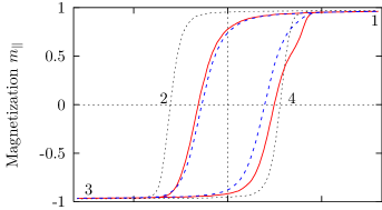
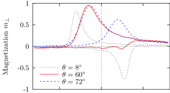
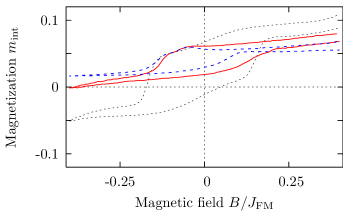
Figure 1: Projection of the magnetization along (upper graph) and perpendicular (central graph) to the applied field $\underline{B}$. The lower graph shows the AFM interface magnetization (along $z$ direction).

Depending on the angle $\theta$ one observes either a symmetric reversal by coherent rotation ($8^{\circ}$), an asymmetric reversal by coherent rotation for the descending branch and a non-uniform mode with zero perpendicular magnetization for the ascending branch ($60^{\circ}$), or symmetric reversal by coherent rotation ($72^{\circ}$) but – in contrast to the usual behavior – with the reversal along the same direction for the descending and ascending branch.

These effects are even more clearly shown in Fig. 2 where the same angular dependence of the magnetization reversal is plotted as $m_{z}$ versus $m_{y}$, with $m_{z}$ ($m_{y}$) denoting the magnetization parallel (perpendicular) to the Ising axis of AFM and FM. Each plot starts at point 1 corresponding to a magnetization with the maximum applied external field $\underline{B}$. Here the spins of the FM are aligned with the external field. With decreasing field $\underline{B}$ the magnetization starts to rotate clockwise and the parallel magnetization will eventually vanish thus yielding the coercive field $B^{-}$ (point 2). For an increasing field the corresponding field value is $B^{+}$ (point 4). When a negative maximum field is applied (point 3) the spins are aligned antiparallel with respect to their initial orientation at point 1.

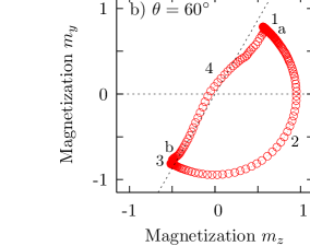
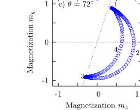
Figure 2: Magnetization $m_{y}$ versus $m_{z}$ for different angles $\theta$; 1 and 3 indicate points with maximum external field $|\underline{B}|$ and 2 and 4 points where $m_{\|}$ vanishes. The horizontal dashed line corresponds to the easy axis of FM and AFM and the other dashed line to the field axis.

For $\theta=8^{\circ}$ (Fig. 2a) we observe mainly coherent rotation for magnetization reversal on both sides of the hysteresis loop. When the external field is either decreased or increased the FM spins first rotate towards their closest easy axis before reversal eventually occurs. Therefore one obtains different signs for the perpendicular magnetization for decreasing and increasing fields, respectively. In Fig. 2b ($\theta=60^{\circ}$) one observes that for a decreasing external field the system behaves as before displaying coherent rotation. When the external field is increased, the system shows an entirely different behavior, though. The contribution of the magnetization perpendicular to the field axis is negligible. Obviously, here we have a highly non-uniform reversal mode with vanishing total magnetization. Increasing $\theta$ even further to $72^{\circ}$ (Fig. 2c) reveals again reversal mainly by coherent rotation on either side of the hysteresis loop with a smaller net contribution $m_{\perp}$ on the increasing branch. Most notably however is the fact that now the rotation occurs via the same side for both branches of the hysteresis loop, in contrast to the reversal for small angles.

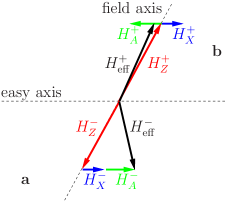
Figure 3: Sketch of the effective field contributions from external field, $H_{Z}$, exchange field of AFM $H_{X}$, and uniaxial anisotropy $H_{A}$ acting on the FM close to the coercive fields $B^{+}$ and $B^{-}$ before the reversal sets in.

For an understanding of these effects we note, that there are three different contributions to the mean effective field $\underline{H}_{\mathrm{eff}}$ acting on the FM during its reversal, namely the exchange field of the AFM, $\underline{H}_{X}=J_{\mathrm{INT}}m_{\mathrm{AFM}}\underline{\hat{z}}$ aligned with the easy axis of the AFM, the external magnetic field, $\underline{H}_{Z}=\underline{B}$, and the anisotropy field $\underline{H}_{A}=2D_{z}m_{\mathrm{FM}}\underline{\hat{z}}$ aligned with the easy axis of the FM, here, also the $z$ axis.

For the particular case shown in Fig. 2b ($60^{\circ}$) these effective field contributions are sketched in Fig. 3 for two characteristic values of the magnetization, a and b in Fig. 2b. As is shown in Fig. 1c), for this value of $\theta$ the magnetization curve of the AFM which is shifted upwards due to the fact that the AFM is in a DS with a surplus magnetization after field cooling nowakPRB02 leads always to a positive effective exchange field $\underline{H}_{X}$. Additionally an effective field coming from the anisotropy of the FM acts on the FM which tries to rotate the magnetization to its closest easy-axis direction. It depends on the sign of the FM magnetization and, consequently, points into different direction on both sides of the hysteresis. The fields labeled with $-$ in Fig. 3 correspond to point a in Fig. 2b, the fields with $+$ to point b. In the first case the effective field has a large angle with the magnetization leading to a strong torque which favors coherent rotation. In the second case the effective field is more aligned with the magnetization which favors non-uniform reversal modes. Note that this is in particular true for $\theta=0^{\circ}$ where the effective field is aligned with the applied field on both sides of the loop. Here, in agreement with the above discussion we observed in the simulations non-uniform reversal modes on both sides. However, we do not show these results here, since we believe that the perfect alignment of field and easy axis is a very special case which hardly will occur in an experimental situation.

The strength of the anisotropy field depends on the projection of $m_{\mathrm{FM}}$ onto the easy axis and decreases with increasing angle $\theta$. When $H_{A}^{+}$ is smaller than $H_{X}^{+}$ the reversal on the ascending loop branch will be over the same side as that of the descending branch (as in Fig. 2c).

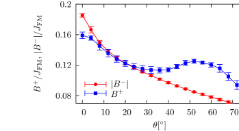
Figure 4: Coercive field values $B^{+}$ and $B^{-}$ versus angle between field and easy axis of FM and AFM.

A finite angle $\theta$ between the applied magnetic field and the easy axis of the AFM can lead to another surprising effect: the possibility of a change of the sign of the bias field when changing this angle. The reason is a different dependence of the coercive fields on $\theta$ due to the different reversal mechanism discussed above. The coercive fields as function of $\theta$ are shown in Fig. 4. For $B^{-}$ the reversal mechanism is always a coherent rotation and its value decreases with $\theta$ monotonically. On the other hand, for $B^{+}$ the behavior is more difficult. Here we found a non-uniform reversal mode for intermediate angles for which $B^{+}$ increases with $\theta$ which may even lead to change of sign of the bias field for certain angles. Note, however, that this requires bias fields which are rather small as compared to the coercive fields, so that this effect might not always be observed.

To summarize, varying the angle between the applied magnetic field and the easy axis of FM and AFM we found either identical or different reversal modes on the ascending and descending branch of the hysteresis loop. For $\theta=60^{\circ}$ the reversal is maximal asymmetric, with a coherent rotation for the descending branch and a non-uniform reversal with zero perpendicular magnetization for the ascending branch. We note, that different angular dependencies are obtained for different system parameters, e. g. varying the exchange constants or the AFM layer thicknesses. For a comparison with experimental situations one should note that in realistic systems the situation might be even more complicated due to i) a twinned or granular structure of the AFM leading to a less well defined anisotropy axis ii) a possible additional angle between easy axis of FM and AFM which in our investigation are identical. However, our investigations show that in general one has to deal with different reversal modes for the ascending and descending branch, respectively, resulting in interesting and even surprising new effects. Furthermore, our model reveals that a twinned crystal structure of the AFM is not necessary for the occurrence of an asymmetry in contrast to what was conjectured earlier fitzsimmonsPRB02 . In corresponding experimental investigations a systematic variation of the angle between the magnetic field and the easy axis of FM and AFM is highly desirable. We expect a deeper insight into the physics of EB from a comparison of those results and our simulations.

References

- (1) J. Nogués and I. K. Schuller, J. Magn. Magn. Mat. 192, 203 (1999).
- (2) A. P. Malozemoff, Phys. Rev. B 35, 3679 (1987).
- (3) D. Mauri, H. C. Siegmann, P. S. Bagus, and E. Kay, J. Appl. Phys. 62, 3047 (1987).
- (4) N. C. Koon, Phys. Rev. Lett. 78, 4865 (1998).
- (5) T. C. Schulthess and W. H. Butler, Phys. Rev. Lett. 81, 4516 (1998).
- (6) M. D. Stiles and R. D. McMichael, Phys. Rev. B 59, 3722 (1999).
- (7) M. Kiwi, J. Mejía-López, R. D. Portugal, and R. Ramírez, Europhys. Lett. 48, 573 (1997).
- (8) P. Miltényi et al., Phys. Rev. Lett. 84, 4224 (2000).
- (9) U. Nowak, A. Misra, and K. D. Usadel, J. Magn. Magn. Mat. 240, 243 (2002).
- (10) U. Nowak et al., Phys. Rev. B 66, 14430 (2002).
- (11) J. Keller et al., Phys. Rev. B 66, 14431 (2002).
- (12) H. T. Shi, D. Lederman, and E. E. C. Fullerton, J. Appl. Phys. 91, 7763 (2002).
- (13) T. Mewes et al., Appl. Phys. Lett. 76, 1057 (2000).
- (14) A. Mougin et al., Phys. Rev. B 63, 60409 (2001).
- (15) A. Misra, U. Nowak, and K. D. Usadel, J. Appl. Phys. 93, 6593 (2003).
- (16) F. Nolting et al., Nature 405, 767 (2000).
- (17) H. Ohldag et al., Phys. Rev. Lett. 86, 2878 (2001).
- (18) M. R. Fitzsimmons et al., Phys. Rev. Lett. 84, 3986 (2000).
- (19) F. Radu et al., J. Magn. Magn. Mat. 240, 251 (2002).
- (20) D. Suess et al., Phys. Rev. B 67, 54419 (2003).
- (21) U. Nowak, in Annual Reviews of Computational Physics IX, edited by D. Stauffer (World Scientific, Singapore, 2001), p. 105.
- (22) M. R. Fitzsimmons et al., Phys. Rev. B 65, 134436 (2002).