On the Evolution of Time Horizons in Parallel and Grid Simulations

Abstract

We analyze the evolution of the local simulation times (LST) in Parallel Discrete Event Simulations. The new ingredients introduced are i) we associate the LST with the nodes and not with the processing elements, and 2) we propose to minimize the exchange of information between different processing elements by freezing the LST on the boundaries between processing elements for some time of processing and then releasing them by a wide-stream memory exchange between processing elements. Highlights of our approach are i) it keeps the highest level of processor time utilization during the algorithm evolution, ii) it takes a reasonable time for the memory exchange excluding the time-consuming and complicated process of message exchange between processors, and iii) the communication between processors is decoupled from the calculations performed on a processor. The effectiveness of our algorithm grows with the number of nodes (or threads). This algorithm should be applicable for any parallel simulation with short-range interactions, including parallel or grid simulations of partial differential equations.

I Introduction

Parallel and grid computations for simulation of spatially-decomposable models with short-range interactions are arguably the most important topic in traditional applied computer science today. This is because of their application to simulations of many models in science, engineering, social science, manufacturing, and economics. We will first concentrate our discussion on parallel discrete event simulations (PDES), and will show the relationship to all short-ranged grid or parallel simulations in the last sections.

PDES are the execution of a single discrete event simulation program on a parallel computer or on a cluster of computers Fuji90 . It is a challenging area of parallel computing and has numerous applications in physics, computer science, economics and engineering. The number of applications are constantly growing in areas where extensive dynamical processes need to be simulated, especially those requiring a huge memory or wall-clock execution time. For such parallel simulations the system to be simulated is broken spatially into disjoint subsystems, and each processing element (PE) performs simulations on a particular subsystem. The simulated system jumps discontinuously from one state to another, these jumps are called an event. Thus the changes of state occur at discrete points in simulated time, although the time is considered to be continuous. The main challenge is to efficiently process with discrete events without changing the order in which the events are processed, i.e. preserving the causality in the simulation. One technique to help preserve causality is to introduce the idea of a local virtual time Jeff85 on a node or PE, which leads to a surface of local simulated times (LST).

For example, consider a kinetic Monte Carlo simulation for a 2d $L$$\times$$L$ ferromagnetic Ising model on a square lattice. The discrete events are spin flips. If the program is to be simulated using $N_{\rm PE}$ processors, each processor may be allocated an equal spatially-disjoint sublattice of spins. The average interval between two flips of the same spin varies for Metropolis-like algorithms from about 3.3 Monte Carlo steps per spin (MCS) at the critical point $T_{\rm c}\approx 2.609$ to 142.9 MCS at the low temperature of $T=0.5$ Over00 . Implementations of such PDES for kinetic Ising models have been performed using both conservative Korn99 and optimistic Over00 methods of preserving causality in the simulations. In the conservative implementation, a PE waits until causality is not violated before it proceeds with its calculations. In the optimistic implementation, if causality may be violated the calculation proceeds using some guess, and if this guess is incorrect the PE must roll back to an earlier state before any causality violations were present.

In this paper we investigate the dynamics of a number of PDES schemes. These parallel schemes are applicable to a wide range of stochastic cellular automata with local dynamics, where the discrete events are Poisson arrivals. We are interested in the evolution of the time horizon formed with the local simulation time (LST) of the nodes. In contrast with the previous work Korn00 ; Kola02 ; Kola03 ; Kola04 , where each PE manages only one node and communication between PEs is implemented according to the conservative scheme Fuji90 , we generalize the scheme so each PE processes a number of nodes which communicate conservatively, whereas nodes from different PEs communicate according to either the conservative or optimistic scenario. The simulated time horizon is analogous to a growing surface. The local time increments of the node correspond to the deposition of some amounts of “material” at the given element of the surface and the efficiency (which is the fraction of non-idling PEs) of the conservative scheme exactly corresponds to the density of local minima in the surface model. It was shown in Korn00 , that the density of the local minima does not vanish when the number of PEs goes to infinity. This remarkable result insures that the simulated time horizon propagates with a nonzero velocity and that the compute phase of the algorithm is asymptotically scalable.

The width of the time horizon in conservative PDES, after an early-time regime and before saturation, diverges with an exponent consistent with the Kardar-Parisi-Zhang one Korn00 . This scaling property is valid for the averages over the ensemble of the surfaces, or for the ensemble of the time horizons in the language of PDES. It is informative however to analyze the dynamics of a single realization of the time horizon as well. A single realization is strongly affected by the surface fluctuations, and the evaluation of a particular surface sometimes loses the full predictability. It is not clear how these fluctuations are connected with the turbulence of the Burgers solitons, although there are some similarity between LST-horizon evolution and the evolution of the surface slope described by noisy Burgers equations Gurbatov ; Chekhlov ; Fog-noisy .

In the original paper Korn00 each PE simulates only one node in a conservative manner. The efficiency of this algorithm is about $1/4$, on average, i.e. one PE out of four is working at any given time. Each PE sends messages to its neighbors about once in four time slices. One way to increase the utilization is to have each node contain a large portion of the lattice, then the utilization can be increased Korn99 ; Kola02 ; Kola03 ; Kola04 .

We analyze here a more efficient implementation of the Korniss et al. idea. Namely, we realize each node as a thread. Threads are distributed among processor elements so each PE is responsible for some number of threads. The threads within one PE communicate using the conservative PDES manner. Communications among threads on the same PE do not require the inter-processor communication latency time (one needs only system calls within a PE), while inter-processor communication requires calls to the I/O routines. Processes communicate within a single PE using system calls of the operating system. Inter-processor communication requires some I/O operations involved in addition to system calls. Threads were invented just to accelerate communications of the partially independent parts of the program. Their communication is supported by the kernel of modern operation systems Threads .

We have two choices for the inter-processor communication: either conservative and optimistic Fuji90 .

With the conservative inter-processor communications, the evolution of the time horizon will be exactly the same as in Korn00 , albeit the utilization would be larger than $1/4$ and close to unity for large enough $\ell$. Here $\ell$ is the number of nodes on a PE, so the system size simulated is $L=\ell N_{\rm PE}$. We assume that the check of the local minima condition (to avoid causality violations) between threads (nodes within a PE) is negligibly small in comparison with the time needed to process the event.

With optimistic inter-processor communications, the evolution of the time horizon becomes more complex. The optimistic scenario Fuji90 assumes that messages were not sent during some given time window. Causality is then checked. In the case where some node proceeds with broken causality, anti-messages have to be sent between processors, the corresponding events are rejected. This leads to a roll-back to an earlier time and state.

The possible scenarios can be understood taking into account the mapping of our problem onto surface growth dynamics. The messages sent by one PE to another are nothing but the boundary conditions in our algorithm. In fact, there are three (and not the two!) possible boundary conditions for the most left and the most right nodes for the chain of nodes within a PE: continuous, free and fixed. Continuous boundary conditions imply that the boundary nodes would follow the causality, taking messages from the neighbor node on the neighbor PE. So, this corresponds to the totally conservative case.

A more interesting solution is with fixed boundaries. In this case, a slope develops at boundaries of each PE. The angle of the slope depends on the mean of the event time intervals and a nearly flat top grows according to the conservative rule. This solution can be interpreted as a fixed soliton of the corresponding Burgers equation.

Free boundary conditions lead to an optimistic implementation of the algorithm. The evolution of the time horizon with the free boundaries have mixed features compared with the algorithms with continuous or fixed boundaries. This boundary condition will be analyzed elsewhere.

The algorithm we discuss here is a new PDES implementation scheme. The main purpose of the paper is a detailed analysis of this PDES algorithm scheme with fixed boundary conditions. The paper is organized as follows. In section II we review briefly the main ideas of PDES and the approach of Korniss et al. Korn00 . In section III we introduce our algorithm and discuss its behavior for simple realizations in one dimension, two dimensions, and for the solution of partial differential equations. We discuss in IV the results and provide a more general overview.

II Conservative PDES

The PDES method is a tool capable of parallelizing any discrete event dynamic algorithm, even those which appear to be intrinsically sequential ones. One example is the development of a kinetic Ising model algorithm by Lubachevsky Luba88 , and its successful implementation Korn99 which preserves the original dynamics of the model.

II.1 PDES and Kardar-Parisi-Zhang equation

Korniss et al. Korn00 developed an approach for the analysis of such algorithms. They mainly considered the case of one-dimensional systems with only nearest-neighbor interactions and periodic boundary conditions. (See ref. KornL00 for two and three-dimensional cases.) Each site of the Ising model is associated with one PE. Consequently the original model has $N_{\rm PE}=L$ PEs simulating $L$ node (or site). The number of nodes per PE are $\ell=1$. Update attempts at each node are independent Poisson processes with the same rate. (In an actual simulation the rate for the kinetic Monte Carlo for the Ising model depends only on the energy change for a single spin flip.) At each PE, the random time interval $\eta_{i}$ between two successive attempts is exponentially distributed.

Let us associate with PE number $i$ the value of a local simulated time $\tau_{i}(t)$, where we denote by $t$ the discrete time of the parallel steps simultaneously performed by each PE. We start with zero LST on all PEs, i.e. $\tau_{i}(0)=0$, $i=1,2,\ldots,L$. For $t\geq 1$ the LST evolves iteratively as

$$\tau_{i}(t+1)=\tau_{i}(t)+\eta_{i}(t) {\rm if} \tau_{i}(t)\leq{\rm min}\left\{\tau_{i-1}(t),\tau_{i+1}(t)\right\};$$

$$\tau_{i}(t+1)=\tau_{i}(t) {\rm else}$$ , (1)

where $\eta_{i}$ are random exponential variables. Each time the PE number $i$ advances in time it sends messages to the right $(i+1)$ and left $(i-1)$ PEs with the time stamp of it’s LST $\tau_{i}(t)$. This insures that the updating process (1) does not violate causality. This category of PDES is called the conservative PDES scenario.

The Korniss et al. algorithm is free of deadlock, since at least the PE with the absolute minimum LST can proceed. The efficiency of the algorithm is the fraction of nonidling PEs and exactly corresponds to the density of local minima of the simulated time horizon.

The iterative process (1) can be rewritten as

$$\tau_{i}(t+1)= \tau_{i}(t)+\Theta\left(\tau_{i-1}(t)-\tau_{i}(t)\right)$$ (2)

$$\times\Theta\left(\tau_{i+1}(t)-\tau_{i}(t)\right)\eta_{i}(t)$$

using the Heaviside step function $\Theta$.

Introducing the local slopes $\phi_{i}=\tau_{i}-\tau_{i-1}$, the density of local minima can be written as

$$u(t)=\frac{1}{L}\sum_{i=1}^{L}\Theta\left(-\phi_{i}(t)\right)\Theta\left(-\phi_{i+1}(t)\right)$$ (3)

and its average

$$\left\langle u(t)\right\rangle=\left\langle\Theta\left(-\phi_{i}(t)\right)\Theta\left(\phi_{i+1}(t)\right)\right\rangle$$ (4)

is the mean velocity of the time horizon, equal to $0.246410(7)$. Hence, the efficiency of the algorithm (in this worst-case scenareo) is about 25 per cent.

It was argued by Korniss et al Korn00 that the coarse-grained slope of time horizon $\hat{\phi}(x,\hat{t})$ in the continuum limit evaluates according to the Burgers equation Kard86

$$\frac{\partial\hat{\phi}}{\partial\hat{t}}=\frac{\partial^{2}\hat{\phi}}{\partial x^{2}}-\lambda\frac{\partial\hat{\phi}^{2}}{\partial x}$$ (5)

and the coarse-grained time-horizon $\hat{\tau}$, $\left(\hat{\phi}=\partial\hat{t}/\partial x\right)$ obeys the Kardar-Parisi-Zhang (KPZ) equation

$$\frac{\partial\hat{\tau}}{\partial\hat{t}}=\frac{\partial^{2}\hat{\tau}}{\partial x^{2}}-\lambda\left(\frac{\partial\hat{\tau}}{\partial x}\right)^{2}\>,$$ (6)

which should be extended with the noise to capture the fluctuations.

II.2 Time horizon evaluation in conservative PDES

The Monte Carlo simulations of the process (1) showed Korn00 that the average width of time horizon

$$\left\langle w^{2}(t)\right\rangle=\frac{1}{L}\left\langle\sum_{i=1}^{L}\left(\tau_{i}(t)-\bar{\tau}(t)\right)^{2}\right\rangle,$$ (7)

where $\bar{\tau}(t)=(1/L)\sum\tau_{i}(t)$, grows for appropriately chosen times (before the LST saturates) as $\left\langle w^{2}(t)\right\rangle\propto t^{2\beta}$ with the exponent $\beta$ close to the KPZ exponent, $\beta$$=$$1/3$. Running a single PDES on a parallel computer the LST horizon develops as a particular realization of the stochastic growth process, not as the average process.

It is known, that the dynamics of solitons in the noisy Burgers equation develops so-called Burgers turbulence Gurbatov ; Chekhlov ; Fog-noisy . Despite the similarity of the width evolution we have been unsuccessful in finding evidence for Burgers turbulence. The tail of the width distribution (Figure 1a of Korniss et al.) may be due to long-lived fluctuations, rather than due to moving solitons. Figure 1 shows the evolution of the time-horizon width for some realizations of this conservative PDES. A large fluctuation occurs in run number 4 at a time $t\approx 68000$. The momentary picture of the time horizon profile shown on Fig. 2 looks like a soliton. Nevertheless, a more detailed analysis is needed to claim that it is indeed a soliton. This evidence would be difficult to obtain, since the noise in the PDES conservative iterative process (2) strongly masks the expected soliton-like behavior.

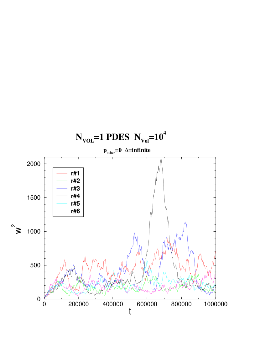
Figure 1: Evolution of the width of the time horizon for several single realizations of conservative PDES. Here there is one site per PE, and $N_{\rm PE}=L=10^{4}$.

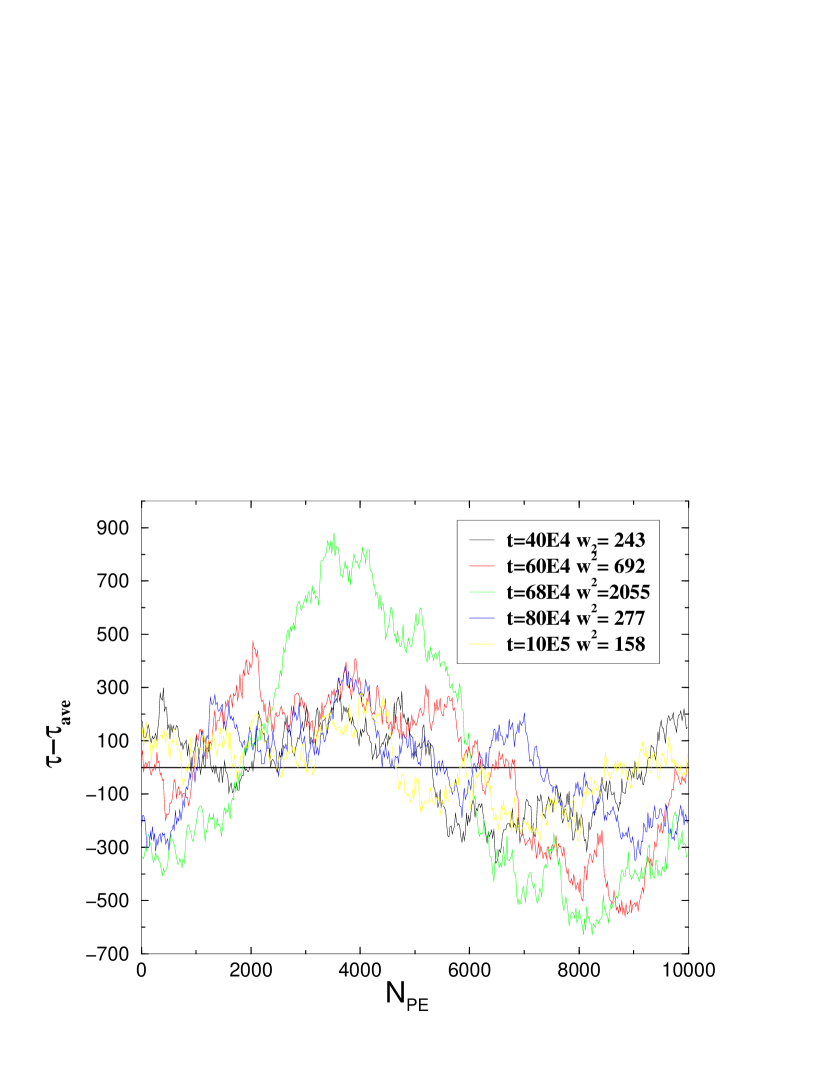
Figure 2: Time horizon profiles at the fixed moments of time for the conservative PDES and $N_{\rm PE}=L=10^{4}$ for run number 4 of Fig. 1.

The large fluctuation in the time horizon profile ($\approx 1600$) is comparable to the system size, $N_{\rm PE}=L=10^{4}$, for the case shown in Fig. 2. In the next section, we will see that the iterative process (2) has steady-state solutions under some boundary conditions, and the time horizon profile shown in Fig. 2 looks similar to it.

III Freeze-and-shift algorithm

III.1 Realizations of PDES.

The conservative PDES algorithm of Korniss et al. is the ideal scheme, in which each PE manages only one process and the LST is associated with the PE. We extend this to a different more general scheme than is present in other publications KornL00 ; Kola02 ; Kola03 ; Kola04 .

Consider the nodes to be vertices of a random graph. The links between the vertices are associated with the possible communications, at least in one direction. Imagine that we can group vertices in clusters, maximizing the connectivity within the cluster and minimizing the number of links between clusters. Let us call those nodes without external links bulk nodes and the rest of the nodes surface nodes. Then, we can map this random graph onto the parallel computer architecture associating one cluster of nodes with the one PE.

Practically, the nodes can be realized as threads Threads . Threads, sometimes called lightweight processes, share the same local memory with the other threads associated with the same PE. Hence, in a practical sense they do not require any extra communication between PEs to communicate with other threads on the same PE. Thus, the communication of the bulk nodes can be organized in the most optimal way, using the conservative PDES implementation.

We have to note that in our approach it is natural to associate the LST with nodes and not with the PEs, in contrast with previous work Korn00 ; KornL00 ; Kola02 ; Kola03 ; Kola04 . All nodes carry its own LST, even those belonging to the same PE.

The communication of surface nodes can be realized in a number of ways.

First, surface nodes can communicate in a conservative manner. The LST horizon will evolve as described by the Korniss et al. scenario discussed in the previous section. Nevertheless, the difference is that the average utilization is not given by $\langle u\rangle$ (see expr. (4)). Let $\ell$ be the number of nodes per PE, so $L=N_{\rm PE}\ell$. The probability of having a chosen node not being at a local minimum of the LST is $1-\langle u\rangle$. Assuming complete randomness among the LST of the nodes, i.e. using a mean-field type of argument Kola04 for non-equilibrium properties of the time-evolving surface, gives that the probability when choosing $\ell$ nodes that all of them are not at a local minimum is $\left(1-\langle u\rangle\right)^{\ell}$. Since a PE can perform an update as long as any of its nodes are at a local minimum, the mean-field argument gives the utilization to be

$$\langle u\rangle=1-\left(1-\langle u\rangle\right)^{\ell}\>.$$ (8)

Our preliminary simulations show that the average utilization for $\ell=1$ depends on the type of noise (all of which have mean noise per step of unity). For uniformly distributed noise it is $\left\langle u\right\rangle_{u}\approx 0.267(4)$. For Gaussian noise it is $\left\langle u\right\rangle_{\rm G}\approx 0.258(5)$. These are to be compared with Poisson noise with $\langle u\rangle=0.246410(7)$. Note that both Gaussian and uniformly distributed noise have an average utilization larger than $1/4$.

In the second realization of PDES, the surface nodes postpone messages within a discrete time window interval $t_{\rm w}$. The system would evaluate in the conservative PDES manner the bulk nodes which lie at a distance from the surface larger than $d\approx\left(\ell-\sqrt{\ell^{2}-4t}\right)/2$ as later given by Expr. (11). After the time $t_{1}\approx\ell^{2}/4$ (see Expr. (9)) the freezing will reach the inner bulk nodes and the evaluation will stop. The system then could not propagate further without an exchange of the messages between PEs to preserve causality. The whole system will at that time be “frozen”. The second idea to implement this algorithm is the fast exchange of the messages. We propose to do that by redistributing nodes between PEs. A simple realization will be discussed below. We call this algorithm the “freeze-and-shift” algorithm (FaS). Note that the FaS algorithm effectively separates the inter-processor communication from the computations progressing on a PE. Thus computer architectures that are capable of simultaneously performing calculations and inter-processor communication can be used effectively, even for problems with fine-grained parallelism. Another potential application of the FaS algorithm is that it should allow simulations with fine-grained parallelism to be performed on calculations on the grid.

The third possible realization is the optimistic scenario of PDES, in which one assumes that all messages come in an order in which causality is not violated. After a discrete time $t_{\rm w}$, one has to check causality and send anti-messages to kill those which violate causality. The process of generating anti-messages can lead to “avalanches” of the time-horizon. These seem to finish with a time horizon profile similar to the one generated by the FaS algorithm introduced above. Clearly, the optimistic scenario is more time consuming: first, the anti-message generation is not a short process; and second, some substantial amount of work on the nodes processed will be rejected. As described on a PE with $\ell$ nodes, the optimistic scenario is some generalization of a combination of the first two scenarios. The understanding of the time horizon avalanche process in the optimistic scenareo can be interesting by itself, but will not be explored in this paper.

III.2 Time horizon evolution for the FaS algorithm

In this subsection, for reasons of clarity, we discuss the simplest case of the FaS algorithm where the nodes effectively form a one-dimensional graph. Despite this simplicity, the one-dimensional case of the FaS algorithm can be applied to the parallel simulation of one-dimensional partial differential equations (see section IV). The one-dimensional FaS algorithm can also be used in simulations of systems that have been organized into disjoint spatial subsystem slices, with the slices forming a one-dimensional graph.

Let us assume there are $\ell$ nodes (or threads) on each of $N_{\rm PE}$ processor elements. For the case of Ising model simulations, each node carries just one spin of the system of $L=\ell N_{\rm PE}$ spins. Nodes within a PE communicate in the conservative manner. The three possible ways of the inter-PE communication correspond to different boundary conditions: the conservative scenario is associated with continuous boundary conditions; the FaS scenario corresponds to fixed boundary conditions; and the optimistic scenario - to free boundary conditions (and associated LST roll-backs).

As we mentioned already, our implementation of conservative PDES is analogous to that of the Korniss et al $\ell=1$ implementation Korn00 and further extensions to larger $\ell$ Kola02 ; Kola03 ; Kola04 . The only difference, and a major difference for algorithm design, is that in our case the LST is associated with the nodes and not with the PEs.

In the case of the FaS algorithm, the evolution of the LST horizon is quite different.

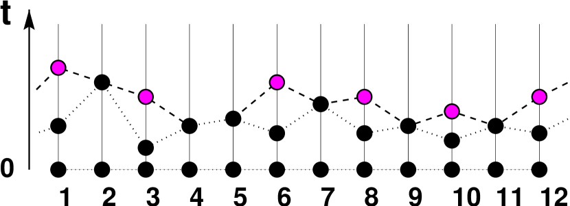
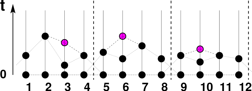
Figure 3: Possible realizations of the first two steps of the time horizon evaluation: Conservative algorithm with $N_{\rm PE}=L=12$ and $\ell=1$ (Top) and the Freeze-and-Shift (FaS) Algorithm with $N_{\rm PE}=3$ with $\ell=4$ nodes each ($L=N_{\rm PE}\ell=12$).

In Fig. 3 the two first steps of the possible evolution of the time horizon are sketched both for the case of the conservative scenario with $\ell=1$ and for the freeze-and-shift (FaS) scenario with $\ell=4$. Initially, at the time $t=0$ all $\tau_{i}=0$. In the first step of PDES all the nodes proceed — the condition (1) is fulfilled for all nodes. The difference between the two scenarious starts just after the first event (time step). In the top of Fig. 3, all the local minima will advance in the conservative scenario. For the frozen boundaries of the FaS algorithm, the left and right boundaries on each PE are fixed, so these minima cannot proceed. As the FaS algorithm progresses, the LST starts to develop a slope with an average angle $\psi$. The average value of this angle depends only on the mean of the noise for a single time slice, with it’s tangent being equal to that mean. This is because proceeding from a frozen node the question is: given that the next node can exceed the value of $\tau$ on the frozen node in the next time step what is the average distance at which its value of $\tau$ freezes ahead of the frozen node’s $\tau$? Since we are using a mean noise of unity, the average angle will be $\psi=\pi/4$ for all types of noise. This is seen in Fig. 4. Note that this profile would also develop if the algorithm always added unity to each updated node, as would be done in simulations of partial differential equations (see later on).

The process of growth will stop at the moment the time horizon reaches the hill knap. This average time can be calculated by assuming that it is given by the same time as the case where each node update advances $\tau$ by one unit. This gives that

$$t_{1}=2\sum_{i=1}^{\ell/2}i\approx\frac{\ell^{2}}{4}\>.$$ (9)

At that time the LST of each individual PE will look like a saw-tooth (Fig. 4). At time $t_{1}$ the entire time horizon will look like a saw with $N_{\rm PE}$ teeth. It is very important to realize that up to that time all PEs were with high probability busy with an efficiency of one .

After a time $t_{1}$ the profile of the time horizon stops developing. Thus the PE can on average perform $t_{1}$ node updates before the LST profile freezes. Figure 4 shows a realization of this frozen steady-state profile. The derivative of the profile $\phi_{i}=\tau_{i+1}-\tau_{i}$ will represent a kink, the soliton-antisoliton pair. Contrary to the Burgers equation Fog-noisy , these kinks are not moving but are in the steady-state. We have an interesting result: by fixing the boundaries we select the soliton-antisoliton solution of equation (2).

The mean value of the LST-horizon for $t\leq t_{1}$ can also be calculated. Consider the non-random case, starting with a flat distribution for $\tau=0$. The time for the LST-horizon to reach a plateau with all middle nodes at the same value of $\tau$ is

$$t=\sum_{i=1}^{\tau}\left(\ell-\tau\right)\approx\tau\ell-\tau^{2}\>.$$ (10)

This equation can be solved for $\tau$ using the quadratic equation and choosing the physical root since $\tau\leq\ell/2$, giving

$$\tau=\left(\ell-\sqrt{\ell^{2}-4t}\right)/2\>.$$ (11)

For this configuration the average value of the LST is

$$\langle\tau\rangle=\frac{\tau(\ell-\tau)}{\ell}\>.$$ (12)

Then substituting for $\tau$ from Eq. (11) gives an expression for the time dependence for $\langle\tau\rangle$ for times $0\leq t\leq t_{1}$. In a similar fashion an expression for the time evolution of $\langle w^{2}\rangle$ can be derived.

Figure 4: Profile of the LST of $\ell=1000$ nodes with fixed boundaries at the leftmost and rightmost positions.

At time $t_{1}$ the LST-horizon is frozen, and the question is how to proceed further with the simulation. The solution we propose is to redistribute the nodes between the PEs. For example, let us shift them by $\ell/2$ to the right (or left), so the tops of the hills (saw-teeth) will be at the boundaries of the processors and fixed for the next time window processing.

Futher evolution of the time horizon is illustrated in Fig. 5. The lowest curve is the LST-horizon depicted on Fig. 4 and cyclically shifted by $\ell/2$. The LST-horizon will grow on average until the time $t_{2}\approx 3t_{1}=3\ell^{2}/4$ at which time the next steady-state frozen solution will be reached (the highest curve in Fig. 5).

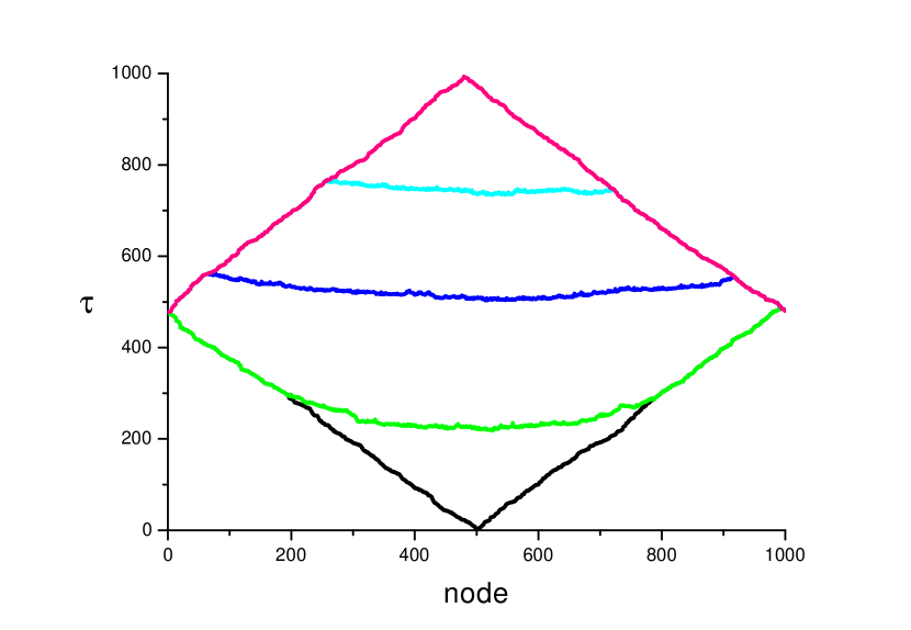
Figure 5: Profile of the LST of $\ell=1000$ nodes at the time $t_{1}$ after shifting by half (bottom line) and at the time values $\approx 1.4t_{1}$, $\approx 1.8t_{1}$, $\approx 2.5t_{1}$, and $3t_{1}$ from the second bottom to the top.

The process can be repeated by alternating freezing of the boundaries for a time window interval not longer than $2t_{1}$ and shifting nodes between PEs by $\ell/2$ for each time window. Figure 6 illustrates this process for $\ell=1000$ nodes and $N_{\rm PE}=5$ for ten shift-cycles with the time window of $2t_{1}$. Consequently there are about $20t_{1}$ time steps (discrete events).

Figure 6: Profile of a LST with $\ell=1000$ nodes in each of the $N_{\rm PE}=5$ PEs.

The square width $w^{2}(t)$ of the time horizon (LST) seems to evolve periodically with time between a minimum and a maximum value. The evidence for this is seen in Fig. 7 in which the LST evolution of $\left\langle w^{2}\right\rangle$ for $\ell=10^{3}$ and $N_{\rm PE}=5$ is shown. For the time between $t=2\times 10^{4}$ and up to the $t=2\times 10^{5}$ the LST-horizon width grows with the effective exponent $z=3/2$, it then stops at the shift moment, and oscillations start. This exponent is not associated with any stochastic process, but reflects the deterministic process of the saw-tooth’s formation according with Expressions (9-12). Probably, the maximum values of the LST width would follow the KPZ exponent, and this is a fruitful subject for future research. Figure 7 seems to show that in the FaS algorithm one can limit (effectively “saturate”) the size of the surface width. Proven ways of saturating the surface width in conservative PDES simulations include imposing a fixed constraint on the width Kola02 and imposing small-world connections between PEs Korn03 . Although the freeze-and-shift method damps out the surface width, much larger studies would be required to see whether or not the governing universality class of the interface is still the KPZ universality class and the FaS algorithm just leads to a coarse-grained length in the KPZ equation.

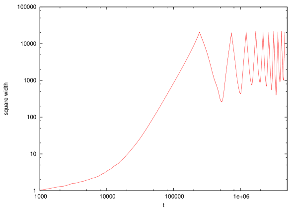
Figure 7: The square of the LST width of the process depicted in Fig. 6.

The time window $t_{\rm w}$ for the freeze-and-shift algorithm can be chosen as any value in the interval $1<t_{\rm w}\leq t_{1}$. We can choose them shorter then $t_{1}$, for example equal to $t_{1}/2$ as shown in Fig. 8 and Fig. 9 for the even and odd shifts, respectively. The difference between the maximum and minimum possible values of the LST will be smaller than in the case of larger $t_{\rm w}$.

Figure 8: Profile of the LST for $\ell=1000$ nodes on each of $N_{\rm PE}=5$ PEs. Curves from bottom to top are the profiles for $t_{\rm w}=\ell$ discrete events at the time moments $t_{k}=(2k-1)\ell$, $2k-1=1,3,5,7,9$.

Figure 9: Profile of the LST of $\ell=1000$ nodes in each of the $N_{\rm PE}=5$ PEs. Curves from bottom to top are the profiles for $t_{\rm w}=\ell$ discrete events at the times $t_{k}=2k\ell$, $2k=2,4,6,8,10$.

III.3 FaS on a two-dimensional lattice

The next interesting realization of the freeze-and-shift algorithm is the application to a two-dimensional model. Suppose we have $N_{\rm PE}$ each of which will simulate a $\ell\times\ell$ block of nodes (spins in kinetic Monte Carlo for the Ising model). The total system size is $L^{2}=N_{\rm PE}\ell^{2}$ where $N_{\rm PE}$ should be a perfect square. We associate $\ell^{2}$ sites (spins) with $\ell^{2}$ threads running on each of the $N_{\rm PE}$ PEs. The evolution of the LST horizon is described by the two-dimensional iterative process (compare with expression (2))

$$\tau_{i,j}(t+1)= \tau_{i,j}(t)+\Theta\left(\tau_{i-1,j}(t)-\tau_{i,j}(t)\right)$$ (13)

$$\times\Theta\left(\tau_{i+1,j}(t)-\tau_{i,j}(t)\right)$$

$$\times\Theta\left(\tau_{i,j-1}(t)-\tau_{i,j}(t)\right)$$

$$\times\Theta\left(\tau_{i,j+1}(t)-\tau_{i,j}(t)\right)\eta_{i}(t)$$

with the product of four theta-functions at the right hand side and $(i,j)$ are coordinates of the lattice edges. For $\ell=1$ one expects that the average speed of time horizon for the conservative PDES scenario will be approximately $\left\langle u_{2}\right\rangle\approx 1/8$, two times slower than in one-dimensional case. Our computer simulation gives $\left\langle u_{2}\right\rangle=0.1205(2)$ for a Poisson distribution of PDES arrival times with unit mean value. This value again depends on the distribution law of the random numbers used.

Figure 10 shows the steady-state solution of process (13) which looks like a pyramid with the slope $1/2$. This solution is achieved at a time given by the volume of the pyramid, $t_{\rm 2-sst}\approx\ell^{3}/12$.

Figure 10: Steady-state profile of the LST on a two-dimensional square lattice with linear number of nodes $\ell=200$.

We have to note that up to the time $t_{\rm 2-sst}$ the efficiency of the FaS algorithm is practically unity. Shifting the nodes between the PEs can now be accomplished in many different ways. Shifting the nodes by $\ell/2$ in both directions of the lattice is equivalent to the sending of postponed messages in the language of PDES. Then, the LST frozen profile will take a time of double $t_{\rm 2-sst}$ before reaching the second frozen steady-state position. Repeating this process of freezing and shifting, we can evolve our nodes in parallel as far as we wish. As in the one-dimensional FaS algorithm, the time between shifting can be any value given by $0<t_{\rm w}\leq t_{\rm 2-sst}$. Note that this shifting can usually be implemented very effectively on modern computers which have fast methods of copying whole blocks of memory between processors, and may have the ability to simultaneously perform calculations and message passing.

III.4 FaS, partial differential equations, grid computing

The discussed algorithms can be effectively applied also to numerical solutions for solving partial differential equations. In this case one has to solve iteratively finite-differences equations defined on the lattice. For simplicity we will discuss partial differential equations of second order in the one-dimensional case. The common form can be written as

$$\psi_{i}(m)=F(\psi_{i}(m),\psi_{i-1}(m),\psi_{i+1}(m),\psi_{i}(m-1),\psi_{i-1}(m-1),\psi_{i+1}(m-1);\Delta,\delta),$$ (14)

where the index $i$ is associated with the space variable, the space increment is $\delta$, and $m$ is associated with the time variable for which the increment is $\Delta$.

We have to divide the entire one-dimensional lattice into $N_{\rm PE}$ pieces, each with $\ell$ lattice nodes, and then associate each piece with a single PE. The LST time increment is equal to $\Delta$, and is not random in this case. We freeze the nodes at the boundaries for each PE. The propagation of the algorithm on each PE will be the normal one, except the nodes that do not know the values of their own or neighboring nodes at both times $m$ and $m+\Delta$ will be frozen. This condition of the frozen boundaries between neighboring PEs will form a LST horizon on each PE. For each time step $\Delta$ the space coordinates of the LST will be $\delta$. If the calculation of the right-hand side of Eq. 14 needs a large time compared with memory shifting between PEs, this algorithm could be very effectively implemented on a parallel computer architecture.

The scheme can be generalized to large dimensions of the lattice, i.e. to the many-dimensional partial differential equations, in the manner demonstrated in the previous subsection for FaS PDES.

Grid computing should enable geographically distributed heterogeneous computations to be performed if appropriate algorithms are available. For previous implementations with fine-grained parallelism, such algorithms are not available. For example, for conservative PDES simulations implemented with one virtual time per PE, the calculation on a particular PE halts at irregular times (whenever the algorithm hits the surface node of the PE). However, conservative PDES implemented with one virtual time per PE allows for an approximately regular and calculable number of time steps $t$ that a PE can perform before it needs to halt to preserve causality. Furthermore, the FaS algorithm allows a decoupling of calculation and the communication. Both of these facts can be important for grid computing. One example is since grid communication paths are used by many people the time for communication between grid computers is not constant, the communication between grid computers can take place without the calculations on a computer having to wait for another computer. Furthermore, the communication may be timed so it is performed when others are historically utilizing the communications network the least (say during nights or weekends). Thus the FaS algorithm should allow grid computations to be performed for PDES simulations and for numerical solutions of partial differential equations.

IV Discussion

We have proposed a new algorithm for parallel discrete event simulations (PDES) which allows for an effective realization on the parallel computers, clusters of computers, and in grid computing. We call this algorithm the FaS (Freeze-and-Shift) algorithm. It effectively decouples the computation phase and communication phase for these parallel computations. This allows, for example, the programmer to utilize fast block-memory-transfer commands. Furthermore, it should allow the efficient simultaneous execution of both computation and communication hardware when they are performed by separate hardware.

There are several essential points of our FaS algorithm. First, we associate a LST with the nodes rather then individual processing elements (PEs). Second, we group the nodes using some rule (see later) and associate each group with a PE (usually the processor running the one process). The nodes are realized as threads, which share the same memory within one process. This allows for a fast realization of the conservative PDES rules within a PE. PEs do not communicate with other PEs for some time interval window $t_{\rm w}$ (the frozen part of the algorithm), and after that time the message exchange is realized as part-of-the-memory shifting between PEs (the shift part of the algorithm). The last part can be very efficiently realized on some parallel architectures. The width of the LST-horizon, which characterizes the difference in the LST between different shifts is under control and depends on the number of nodes $\ell$ per PE. The FaS algorithm guaranties the efficiency of the simulations and idleness of PEs should be nearly equal to zero for balanced simulations.

The general scheme can be sketched as in Fig. 11, where we have partitioned the nodes into groups (associated with PEs during the freeze part of the FaS algorithm) and we freeze development of those nodes within the interfaces. The efficiency of the algorithm depends on the smallness of the ratio of the interface area to the bulk area, and on the new (alternating) interface area we have to create by the shifting of nodes between PEs (the alternating partitioning of the node manifold).

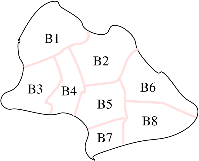
Figure 11: Nodes manifold partitioning into eight groups of bulk nodes, each associated with a single PE during the frozen phase of the FaS algorithm.

Analysis of several realizations demonstrate the efficiency of the general idea of the FaS algorithm. Actual implementations on parallel computers, heterogeneous compute clusters, and computer grids for problems of interest will determine the ultimate usefulness of the FaS algorithm.

- (1) R.M. Fujimoto, Comm. ACM, 33 (1990) 31.
- (2) D.R. Jefferson, Assoc. Comput. Mach. Trans. Programming Languages and Systems 7, (1985) 404.
- (3) P.M.A. Sloot, B.J. Overeinder, and A. Schoneveld, Comp. Phys. Comm., 142 (2001) 76; B.J. Overeinder, PhD Thesis, Univ. of Amsterdam, 2000.
- (4) G. Korniss, M.A. Novotny, and P.A. Rikvold, J. Comput. Phys., 153 (1999) 488.
- (5) G. Korniss, Z. Toroczkai, M.A. Novotny, and P.A. Rikvold, Phys. Rev. Lett., 84 (2000) 1351.
- (6) A. Kolakowska, M.A. Novotny, and G. Korniss, Phys. Rev. E 67 (2002) 046703.
- (7) A. Kolakowska, M.A. Novotny, and P.A. Rikvold, Phys. Rev. E 68 (2003) 046705.
- (8) A. Kolakowska and M.A. Novotny, Phys. Rev. E, submitted, preprint cond-mat/0311015.
- (9) S.N. Gurbatov, A.N. Malakhov, A.I. Saichev, Nonlinear random waves and turbulence in nondispersive media: waves, rays, particles, (Manchester University Press, Manchester, 1991)
- (10) A. Chekhlov, and V. Yakhot, Phys. Rev. E 51 (1995) R2739.
- (11) H.C. Fogedby, Phys. Rev. E., 57 (1998) 4943.
- (12) A.S. Tanenbaum, Modern Operation Systems. (Prentice Hall, Upper Saddle River, 2001).
- (13) B.D. Lubachevsky, Complex Syst., 1 (1987) 1099.; J. Comput. Phys., 75 (1988) 103.
- (14) G. Korniss, M.A. Novotny, Z. Toroczkai, and P.A. Rikvold, in Computer Simulation Studies in Condensed Matter Physics XIII, editors D.P. Landau, S.P. Lewis, and H.-B. Schüttler (Springer Verlag, Heidelberg, 2001), p. 183.
- (15) M. Kardar, G. Parisi, and Y.-C. Zhang, Phys. Rev. Lett., 56 (1986) 889.
- (16) G. Korniss, M.A. Novotny, H. Guclu, Z. Toroczkai, and P.A. Rikvold, Science 299 (2003) 677.