Dilute Fermi gas: kinetic and interaction energies

Abstract

A dilute homogeneous 3D Fermi gas in the ground state is considered for the case of a repulsive pairwise interaction. The low-density (dilution) expansions for the kinetic and interaction energies of the system in question are calculated up to the third order in the dilution parameter. Similar to the recent results for a Bose gas, the calculated quantities turn out to depend on a pairwise interaction through the two characteristic lengths: the former, $a$, is the well-known s-wave scattering length, and the latter, $b$, is related to $a$ by $b=a-m(\partial a/\partial m)$, where $m$ stands for the fermion mass. To take control of the results, calculations are fulfilled in two independent ways. The first involves the Hellmann-Feynman theorem, taken in conjunction with a helpful variational theorem for the scattering length. This way is used to derive the kinetic and interaction energies from the familiar low-density expansion of the total system energy first found by Huang and Yang. The second way operates with the in-medium pair wave functions. It allows one to derive the quantities of interest“from the scratch”, with no use of the total energy. An important result of the present investigation is that the pairwise interaction of fermions makes an essential contribution to their kinetic energy. Moreover, there is a complicated and interesting interplay of these quantities.

I Introduction

Recent experiments with magnetically trapped alkali atoms significantly renewed interest in properties of quantum gases. As it is known, the initial series of these experiments concerned a Bose gas (${}^{87}Rb$ ander , ${}^{23}Na$ davis , and ${}^{7}Li$ brad ) and resulted in extensive reconsiderations and new investigations in the field of the Bose-Einstein condensation. In so doing theoretical and experimental observations were made that not only confirmed conclusions made more than forty years ago but also provided a new horizon of the boson physics. In particular, one should point out good agreement of the results of solving the Gross-Pitaevskii equation derived in 1960s gp with experimental data on the density profiles of a trapped Bose gas hau . The so-called release energy measured in the experiments with rubidium was also found to be in good agreement with theoretical expectations based on the time-dependent Gross-Pitaevskii equation hol . Among new theoretical achievements the exact derivation of the Gross-Pitaevskii energy functional liebA can be mentioned along with the proof that a Bose gas with repulsive interaction is $100\%$ superfluid in the dilute limit liebB . As to the experimental innovations, observations of interference of two Bose condensates andrews ; kett is a good example (for interesting theoretical details see the papers cirac , devr and reviews pit ,legett ).

The first communications concerning experiments with trapped fermionic atoms appeared in the literature about three years ago marco when a temperature near $0.4T_{f}$ was claimed to be reached for a trapped ${}^{6}Li$, where $T_{f}$ is the temperature below which the Fermi statistics is of importance. Nowadays the temperatures close to $0.2T_{f}$ schreck and $0.5T_{f}$ hadzibabic are reported for the ${}^{6}Li$-vapor. Whereas atoms of fermionic ${}^{40}K$ were recently cooled down to $0.3T_{f}$ roati . So, the regime of the degenerate Fermi gas is already under experimental study. In view of this fact, reconsideration of the basic aspects of the theory of a dilute uniform Fermi gas in the ground state is of importance.

In the present paper a dilute Fermi gas with repulsive pairwise interaction is under consideration. Why the situation of a repulsive Fermi gas is of interest whereas the $s-$wave scattering length is negative for ${}^{6}Li$ stoof and, most likely, for ${}^{40}K$ roati so that a trapped ${}^{6}Li$ is considered as a good candidate for observation of BCS-like transition stoof ; combescot ; houbiers ? The point is that the experiments can produce (and is now producing) the temperatures at which the BCS pairing does not occur yet. So, at these temperature a Fermi gas with attractive pairwise interaction is close enough in properties (with the corrections of $O((T/T_{f})^{2})$, where $T/T_{f}\approx 0.2$) to a repulsive Fermi gas in the ground state. Of course, with one obvious alteration: the positive $s-$wave scattering length should be replaced by a negative one in the final expressions (see, for example, stoof ). Thus, the experiments with magnetically trapped atoms of ${}^{6}Li$ and ${}^{40}K$ offer exciting possibility of exploring the both superfluid and normal states of a Fermi gas. In addition, the most recent publications ohara ; bourdel demonstrate that there exists interesting possibility of ruling the scattering length of ${}^{6}Li$ which varies in a wide range of values, from negative to positive ones, when a magnetic field is imposed on the system.

The particular problem to be investigated here concerns the kinetic $E_{\rm kin}$ and interaction $E_{\rm int}$ energies of a uniform dilute 3D Fermi gas in the ground state and with a repulsive interparticle potential. This problem is connected with a more general question related to all the quantum gases. The question is if the pairwise interaction of quantum particles makes contribution to the kinetic energy of a quantum gas or not? It is well-known that for a classical imperfect gas the pairwise interaction does not make any contribution to the kinetic energy. The usual expectations regarding the kinetic energy of dilute quantum gases comes from the pseudopotential approach. According to these expectations the kinetic energy of a dilute quantum gas is not practically affected by the pairwise interaction. It means that taken in the leading order of the expansion in the dilution parameter, the total system energy of a ground-state Bose gas coinsides with the interaction one if calculated with the pseudopotential (see Refs. pit ; shanA ; shanB ). For the Fermi case the same approach dictates that the kinetic energy does not include terms depending on the pairwise potential in the leading and next-to-leading orders of the dilution expansion (see Ref. vichi and Eqs. (24) and (25) below). In other words, in what concerns relation between the kinetic and interaction energies, a quantum gas is very similar to a classical one from the pseudopotential viewpoint. However, this result was proved to be wrong. An adequate and thorough procedure of calculating $E_{\rm kin}$ and $E_{\rm int}$ of a cold dilute Bose gas has been recently developed in Refs. shanA ; shanB . It proves that the pairwise interaction in a Bose gas has a strong effect on the kinetic energy. Moreover, there are quite real situations when the kinetic energy of a uniform dilute Bose gas is essentially more than the interaction one! It is now necessary to clarify this situation in the Fermi case. The more so, that the interaction and kinetic energies of imperfect trapped quantum gases are now under experimental study vichi ; bourdel . Thus, the aim of the present publication is to generalize the procedure developed in shanA ; shanB to the Fermi case.

The paper is organized as follows. The Section II presents the kinetic and interaction energy of a ground-state repulsive Fermi gas found with the Hellmann-Feynman theorem on the basis of an auxiliary variational relation given in Refs. shanA ; shanB . The Section III is to consider the derived expressions in various regimes: from a weak coupling to a strong one. This is needed to discuss the failure of the pseudopotential approach in operating with $E_{\rm kin}$ and $E_{\rm int}$. Derivation of $E_{\rm kin}$ and $E_{\rm int}$ in Section 2 is simple but rather formal so that some questions can remain. This is why Sections IV and V give a more physically sound way of calculating the kinetic and interaction energies. This way invokes a method developed in the papers shanA ; shanB and dealing with the pair wave functions, which allows one to go in more detail concerning the microscopic features of dilute quantum gases.

II Hellmann-Feynman theorem

Let us consider the system of $N$ identical fermions placed in a box with the volume $V$ and ruled by the following Hamiltonian:

$$\hat{H}=-\sum_{i}\frac{\hbar^{2}}{2m}\nabla^{2}_{i}+\sum_{i>j}V(|{\bf r}_{i}-{\bf r}_{j}|)$$ (1)

with the pairwise interaction $V(r)=\gamma\Phi(r)$, where $\gamma>0$ is the coupling constant and $\Phi(r)>0$ stands for the interaction kernel ($r=|{\bf r}|$). Below the particle spin is assumed to be $s=1/2$ note1 . The ground-state energy of the system in question $E=\langle 0|\hat{H}|0\rangle$ obeys the well-known relation

$$\delta E=\langle 0|\delta\hat{H}|0\rangle$$ (2)

called the Hellmann-Feynman theorem, $\delta E$ and $\delta\hat{H}$ being infinitesimal changes of $E$ and $\hat{H}$. An advantage of this theorem is that it yields important relations connecting the total ground-state energy $E$ with the kinetic $E_{\rm kin}$ and interaction $E_{\rm int}$ energies. These relations read

$$-m\frac{\partial E}{\partial m}=\Bigl{\langle}0\Bigl{|}-\sum_{i}\frac{\hbar^{2}}{2m}\nabla^{2}_{i}\Bigr{|}0\Bigr{\rangle}=E_{\rm kin},$$ (3)

$$\gamma\frac{\partial E}{\partial\gamma}=\Bigl{\langle}0\Bigl{|}\sum_{i>j}V(|{\bf r}_{i}-{\bf r}_{j}|)\Bigr{|}0\Bigr{\rangle}=E_{\rm int}.$$ (4)

If the dependence of the ground-state energy on the coupling constant and particle mass were known explicitly, one would readily be able to calculate $E_{\rm kin}$ and $E_{\rm int}$ by means of Eqs. (3) and (4). However, it is not the case as a rule, and the dependence is usually given only implicitly.

In the situation of the repulsive Fermi gas the dependence of the ground-state energy on $\gamma$ and $m$ is indeed known only implicitly. According to the familiar result of Huang and Yang hy found with the pseudopotential approach but then reproduced within the boundary collision expansion method ly beyond any effective-interaction arguments, the energy per fermion $\varepsilon=E/N$ reads

$$\varepsilon=\frac{3\hbar^{2}k^{2}_{F}}{10m}\biggl{[}1+\frac{10}{9\pi}k_{F}a+\frac{4}{21\pi^{2}}(11-2\ln 2)k^{2}_{F}a^{2}\biggr{]},$$ (5)

which is accurate to the terms of order $k^{2}_{F}a^{2}$. In Eq. (5) $a$ stands for the $s-$wave scattering length, $k_{F}$ is the Fermi wavenumber given by

$$k_{F}=(3\pi^{2}n)^{1/3},$$ (6)

where $n=N/V$, and the thermodynamic limit $N\to\infty,\;V\to\infty,\;n=N/V\to const$ is implied. Inserting Eq. (5) in Eqs. (3) and (4), one can arrive at

$$\varepsilon_{\rm kin}=$$

$$=\varepsilon-\frac{3\hbar^{2}k^{2}_{F}}{10a}\,\frac{\partial a}{\partial m}\biggl{[}\frac{10}{9\pi}k_{F}a+\frac{8}{21\pi^{2}}(11\!-\!2\ln 2)k^{2}_{F}a^{2}\biggr{]},\quad$$ (7)

$$\varepsilon_{\rm int}\!=\!\frac{3\hbar^{2}k^{2}_{F}}{10ma}\,\gamma\frac{\partial a}{\partial\gamma}\biggl{[}\frac{10}{9\pi}k_{F}a+\frac{8}{21\pi^{2}}(11\!-\!2\ln 2)k^{2}_{F}a^{2}\biggr{]},\quad$$ (8)

where $\varepsilon_{\rm kin}=E_{\rm kin}/N$ and $\varepsilon_{\rm int}=E_{\rm int}/N$. Hence, to derive the kinetic and interaction energies from Eq. (5) with the help of the Hellmann-Feynman theorem, we should have an idea concerning the derivatives of $a$ with respect to the particle mass $m$ and coupling constant $\gamma$. As $E=E_{\rm kin}+E_{\rm int}$, then from Eqs. (7) and (8) it follows that

$$m\,\partial a/\partial m=\gamma\,\partial a/\partial\gamma.$$ (9)

This property of the derivatives becomes clear if we remind that in the $3D$ case the $s-$wave scattering length is given by

$$a=\frac{m\gamma}{4\pi\hbar^{2}}\int d^{3}r\varphi(r)\Phi(r),$$ (10)

where $\varphi(r)$ obeys the the two-body Schrödinger equation in the center-off-mass system:

$$-(\hbar^{2}/m\gamma)\nabla^{2}\varphi(r)+\Phi(r)\varphi(r)=0.$$ (11)

The pair wave function $\varphi(r)$ represents the zero-momentum scattering state, and $\varphi(r)\to 1$ when $r\to\infty$. The scattering part of the pair wave function given by the definition $\varphi(r)=1+\psi(r)$ is specified by the following asymptotic behavior:

$$\psi(r)\to-a/r\quad(r\to\infty).$$ (12)

Note once more that the pairwise potential involved in Eqs. (10) and (11) is $V(r)=\gamma\Phi(r)$ but not $\Phi(r)$ which is the repulsive interaction kernel. As it is seen from Eqs. (10) and (11), the scattering length depends on the particle mass and coupling constant through the product $m\gamma$. Hence, to use Eqs. (7) and (8) we should know the derivative of $a$ with respect to $m\gamma$.

This derivative can be found with very useful variational theorem proved in the papers shanA ; shanB . After small algebra the result of this theorem is rewritten in the following form:

$$\delta a=\frac{\delta(m\gamma)}{4\pi\hbar^{2}}\int d^{3}r\varphi^{2}(r)\Phi(r),$$ (13)

where, remind, $\varphi(r)$ is a real quantity. In view of crucial importance of this theorem, let us make an explaining remark concerning the proof. The key point here is to represent Eq. (10) as

$$a=\frac{m\gamma}{4\pi\hbar^{2}}\int d^{3}r\varphi^{2}(r)\Phi(r)+\frac{1}{4\pi}\int d^{3}r|\nabla\psi(r)|^{2},$$ (14)

which is realized with the help of Eqs. (11), (12) and $\nabla(\psi\nabla\psi)=\nabla\psi\;\nabla\psi+\psi\nabla^{2}\psi$. So, from Eq. (13) one gets

$$m\partial a/\partial m=\gamma\partial a/\partial\gamma=a-b,$$ (15)

where the additional characteristic length $b>0$ is of the form

$$b=\frac{1}{4\pi}\int d^{3}r|\nabla\psi(r)|^{2}.$$ (16)

Emphasize that $b$ can not be represented as a function of $a$ in principle, and the ratio $b/a$ depends on a particular shape of a pairwise potential involved. Now we need nothing more to calculate the kinetic and interaction energies of the uniform repulsive Fermi gas in the ground state. Equations (7) and (8) taken in conjunction with Eq. (15), result in the following expressions:

$$\varepsilon_{\rm kin}\!= \!\frac{3\hbar^{2}k^{2}_{F}}{10m}\biggl{[}1+\frac{10}{9\pi}k_{F}b$$ (17)

$$+\frac{4}{21\pi^{2}}(11\!-\!2\ln 2)\left(2\frac{b}{a}-1\right)k^{2}_{F}a^{2}\biggr{]},$$

$$\varepsilon_{\rm int}\!= \!\frac{3\hbar^{2}k^{2}_{F}}{10m}\left(1-\frac{b}{a}\right)\!$$ (18)

$$\times\biggl{[}\frac{10}{9\pi}k_{F}a+\frac{8}{21\pi^{2}}(11\!-\!2\ln 2)k^{2}_{F}a^{2}\biggr{]},$$

whose sum is, of course, equal to Eq. (5). We again have series expansions in $k_{F}a$ but with coefficients depending on the ratio $b/a$.

III From weak to strong coupling

To go in more detail concerning Eqs. (17) and (18), let us consider them in various regimes. We speak about the week coupling when the interaction kernel $\Phi(r)$ is integrable and the coupling constant $\gamma\ll 1$. The integrable kernel with $\gamma\gg 1$ and a singular pairwise interaction like the hard-sphere potential are related to the strong-coupling regime. The expansion parameter $k_{F}a$ involved in the expressions mentioned above corresponds to the dilution limit $k_{F}\to 0$. In this situation one is able to operate with Eq. (5) in the both weak- and strong-coupling cases. However, for the weak coupling $k_{F}a$ is small even beyond the dilute regime due to $a\propto\gamma\ll 1$. This is why Eq. (5) can be used and rearranged in such a way that to derive the weak-coupling expansion for $\varepsilon$.

In the weak-coupling regime the scattering length $a$ is given by the Born series:

$$a=a_{0}+a_{1}+\ldots$$ (19)

with

$$a_{0}=\frac{m\gamma}{4\pi\hbar^{2}}\Phi(k=0),\;a_{1\!}=\!-\frac{m\gamma^{2}}{4\pi\hbar^{2}}\int\frac{\mbox{d}^{3}k}{(2\pi)^{3}}\frac{\Phi^{2}(k)}{2T_{k}},$$ (20)

where $T_{k}=\hbar^{2}k^{2}/(2m)$, and $\Phi(k)$ is the Fourier transform of the interaction kernel ( for more detail see Ref. brue ). Inserting Eq. (19) in Eq. (5), one gets the following expression:

$$\varepsilon= \frac{3\hbar^{2}k^{2}_{F}}{10m}\Biggl{[}1+\frac{10}{9\pi}k_{F}a_{0}$$ (21)

$$+\biggl{(}\frac{10}{9\pi}k_{F}a_{1}+\frac{4}{21\pi^{2}}(11\!-\!2\ln 2)k^{2}_{F}a_{0}^{2}\biggr{)}\Biggr{]},$$

where terms of order $\gamma^{3}$ are ignored. Due to Eq. (20) the dependence of Eq. (21) on the particle mass and coupling constant is known explicitly. Hence, one can readily employ the Hellmann-Feynman theorem that, taken together with Eq. (21), yields

$$\varepsilon_{\rm kin}= \frac{3\hbar^{2}k^{2}_{F}}{10m}\Biggl{[}1-$$ (22)

$$-\biggl{(}\frac{10}{9\pi}k_{F}a_{1}+\frac{4}{21\pi^{2}}(11\!-\!2\ln 2)k^{2}_{F}a_{0}^{2}\biggr{)}\Biggr{]},$$

$$\varepsilon_{\rm int}= \frac{3\hbar^{2}k^{2}_{F}}{10m}\Biggl{[}\frac{10}{9\pi}k_{F}a_{0}$$ (23)

$$+\biggl{(}\frac{20}{9\pi}k_{F}a_{1}+\frac{8}{21\pi^{2}}(11\!-\!2\ln 2)k^{2}_{F}a_{0}^{2}\biggr{)}\Biggr{]}.$$

So, the derived results suggest that the pairwise interaction influences the both kinetic and interaction energies of a Fermi gas. In the weak-coupling regime the major part of the $\gamma$-dependent contribution to Eq. (21) is related to $E_{\rm int}$, this part being proportional to $\gamma$. While the terms of order $\gamma^{2}$ appear in both $E_{\rm kin}$ and $E_{\rm int}$. This conclusion meets usual expectations according to which the contribution to the mean energy coming from the pairwise potential is mostly the interaction energy for dilute quantum gases (see, for example, Refs. pit ; stoof and the discussion in Introduction of the paper shanA ). On the contrary, beyond the weak-coupling regime the situation with $E_{\rm kin}$ and $E_{\rm int}$ turned out to be rather curious and differs significantly from that of the weak-coupling case. However, before any detail let us discuss the pseudopotential predictions for $E_{\rm kin}$ and $E_{\rm int}$ being the basis of usual speculations involving the kinetic and interaction energies of quantum gases beyond the weak-coupling regime.

At present the customary way of operating with the thermodynamics of a dilute cold Fermi gas with repulsive pairwise potential is based on the effective-interaction procedure: one is able to use either the $t-$matrix formulation like in the Galitskii original paper gal or the pseudopotential scheme applied in the classical work of Huang and Yang hy . In the dilution limit the $t-$matrix is reduced to $t=4\pi\hbar^{2}a/m$, which yields the momentum-independent result $4\pi\hbar^{2}a/m$ for the Fourier transform of the effective interaction. This is why one is able not to make essential difference between these two effective-interaction formulations both referred to as the pseudopotential approach here. The key point of this approach is that to go beyond the weak-coupling regime, one should replace the Fourier transform of the pairwise interaction $\Phi(k)$ by the quantity $4\pi\hbar^{2}a/m$ in all the expressions related to the weak-coupling approximation. In so doing, some divergent integrals appear due to ignorance of the momentum dependence of the $t-$matrix. Indeed, substituting $t=4\pi\hbar^{2}a/m$ for $\Phi(k)$ in Eq. (14), one gets a divergent quantity $a_{1}\propto\int\mbox{d}^{3}k/2T_{k}$ that makes contribution to the total energy of the system. To derive the classical result of Huang and Yang, the divergent term proportional to $a_{1}$ should be removed, which is usually fulfilled via a regularization procedure simulating the momentum dependence of the $t-$matrix. In the pseudopotential scheme of Huang and Yang this corresponds to use of the effective interaction $(4\pi\hbar^{2}a/m)\delta(r)(\partial/\partial r)r$ rather than $(4\pi\hbar^{2}a/m)\delta(r)$. From this one can learn that to generalize Eqs. (21), (22) and (23) to the situation of a finite coupling constant, one should replace $a_{0}$ by $a$ and remove all the terms depending on $a_{1}$ in the mentioned equations. This yields Eq. (5) and the following pseudopotential predictions for the kinetic and interaction energies:

$$\varepsilon^{(\rm ps)}_{\rm kin}=\frac{3\hbar^{2}k^{2}_{F}}{10m}\biggl{[}1-\frac{4}{21\pi^{2}}(11\!-\!2\ln 2)k^{2}_{F}a^{2}\biggr{]} ,\quad$$ (24)

$$\varepsilon^{(\rm ps)}_{\rm int}=\frac{3\hbar^{2}k^{2}_{F}}{10m}\biggl{[}\frac{10}{9\pi}k_{F}a+\frac{8}{21\pi^{2}}(11\!-\!2\ln 2)k^{2}_{F}a^{2}\biggr{]} .\quad$$ (25)

Note that these results can be derived in another way as well. For example, the first term in Eq. (25) can readily be reproduced with the pseudopotential in the Hartree-Fock approximation (see Ref. hy and the next section of the present paper). From Eqs. (24) and (25) one could conclude that the second term in Eq. (5) is related to the interaction energy, and, hence, the contribution to the mean energy of a dilute cold Fermi gas coming from the pairwise potential is mainly the interaction energy. However, now we know that actually it is not the case. So, one should be careful with the pseudopotential procedure which has serious limitations in spite of the correct result for the mean energy. Here it is worth noting that the pseudopotential scheme preserves some features of the weak-coupling regime even being applied in the strong-coupling case. This concerns the relation between the kinetic and interaction energy for both a dilute Fermi ground-state gas and a Bose one shanA ; shanB . The same problem appears when the pseudopotential is used to calculate the two-particle Green function in a Bose gas, which manifests itself in abnormal short-range boson correlations shanA . Similar troubles can also be expected for the two-fermion Green function.

Now let us consider Eqs. (17) and (18) beyond the weak-coupling regime, the ratio $b/a$ being of special interest. We start with the simplified situation of penetrate-able spheres that are specified by the interaction kernel

$$\Phi(r)=\left\{\begin{array}[]{rr}\Phi&{\rm if}\quad r\leq r_{0},\\[2.84526pt] 0&{\rm if}\quad r>r_{0}.\end{array}\right.$$ (26)

Inserting Eq. (26) in Eq. (11), one can find

$$\varphi(r)=\left\{\begin{array}[]{rr}2A\sinh(\alpha r)/r&{\rm if}\quad r\leq r_{0},\\[2.84526pt] 1-a/r&{\rm if}\quad r>r_{0},\end{array}\right.$$ (27)

where $\alpha^{2}=m\gamma\Phi/\hbar^{2}\;(\Phi>0)$ and $A$ is a constant. Equation (27) taken together with the usual boundary conditions at $r=r_{0}$ leads to

$$a=r_{0}\Bigl{[}1-\tanh(\alpha r_{0})/(\alpha r_{0})\Bigr{]}$$ (28)

and

$$b\!=\!r_{0}\!\left[1\!-\!\frac{1}{2}\Bigl{(}3\tanh(\alpha r_{0})/(\alpha r_{0})\!-\!{\rm csch}(\alpha r_{0})\Bigr{)}\right]\!,$$ (29)

where ${\rm csch}(x)=1/\cosh^{2}(x)$. One can readily check that in the weak-coupling regime, when $\alpha r_{0}\propto\gamma^{1/2}\to 0$, Eqs. (28) and (29) are reduced to

$$a\simeq\frac{1}{3}\alpha^{2}r_{0}^{3}\propto\gamma,\quad b\simeq\frac{2}{15}\alpha^{4}r_{0}^{5}\propto\gamma^{2}$$ (30)

and, hence, $b\ll a$. This means that the next-to-leading term in the expansion in $k_{F}a$ given by Eq. (5) is mostly the interaction energy, as it was mentioned above. On the contrary, in the strong-coupling regime, when $\alpha r_{0}\to\infty$, Eqs. (28) and (29) give

$$a\to r_{0},\quad b\to r_{0}.$$ (31)

Hence, $b/a\to 1$, and the ground-state energy of a dilute Fermi gas with the hard-sphere interaction is exactly kinetic! Note that the same conclusion is valid for a dilute Bose gas of the hard spheres shanA ; shanB ; liebC .

Another, a more realistic example concerns a situation when the interaction kernel combines a short-range repulsive sector with a long-range attractive one. Here we are especially interested in a negative scattering length. It is usually considered (see, e.g., gora ) that for alkali atoms one can employ the following approximation:

$$\Phi(r)=\left\{\begin{array}[]{cc}+\infty&{\rm if}\quad r\leq r_{0},\\[2.84526pt] -C/r^{6}&{\rm if}\quad r>r_{0}.\end{array}\right.$$ (32)

The scattering length for the pair interaction kernel (32) is of the form (see Ref ties )

$$a/r_{c}=\Gamma(3/4)J_{-1/4}(x)/\bigl{[}2\Gamma(5/4)J_{1/4}(x)\bigr{]},$$ (33)

where $x\!=\!r_{c}^{2}/(2r_{0}^{2}),\;r_{c}\!=\!(m\gamma C/\hbar^{2})^{1/4}$, whereas $J_{\nu}(x)$ and $\Gamma(z)$ denote the Bessel function and the Euler gamma-function. It is known that $J_{\nu}(x)\simeq x^{\nu}/[2^{\nu}\Gamma(1+\nu)]$ for $x\to 0$. Therefore, Eq. (33) reduces to $a=r_{0}$ in this limit. In other words, when the attractive sector is “switched off”, we arrive at the hard-sphere result discussed in the previous paragraph of the present section. For $x>0$ the scattering length (33) is a decreasing function of $x$ with the complicated pattern of behaviour specified by the infinite set of singular points $\{x^{(1)}_{\infty},\;x^{(2)}_{\infty},\;x^{(3)}_{\infty},\ldots\}$. These points are the zeros of $J_{1/4}(x)$ so that $a\to-\infty$ when $x\to x^{(i)}_{\infty}-0$ and $a\to+\infty$ when $x\to x^{(i)}_{\infty}+0$. In addition, there is also the infinite sequence of the zeros of the scattering length $\{x^{(1)}_{0},\;x^{(2)}_{0},\;x^{(3)}_{0},\ldots\}$ being the zeros of $J_{-1/4}(x)$. Note that $x^{(i)}_{0}<x^{(i)}_{\infty}<x^{(i+1)}_{0}$. Keeping in mind this information and Eq. (33), we can explore the ratio $b/a$ for the pair interaction kernel (32). Equation (33) leads to

$$\gamma\partial a/\partial\gamma=D\sqrt{x}\,\Bigl{[}J_{-1/4}(x) /\bigl{(}2J_{1/4}(x)\bigr{)}$$ (34)

$$-\,\sqrt{2}/\bigl{(}\pi J^{2}_{1/4}(x)\bigr{)}\Bigr{]}.$$

with $D=r_{0}\Gamma(3/4)/[2^{3/2}\Gamma(5/4)]$. Note that to derive Eq. (34), the useful formula

$$J_{\nu+1}(x)J_{-\nu}(x)+J_{\nu}(x)J_{-(\nu+1)}(x)\!=\!-\,2\sin(\pi\nu)/(\pi x)$$

should be applied. Equation (34), taken in conjunction with Eq. (15), yields

$$b/a=3/4+1/\bigl{[}\pi\sqrt{2}J_{1/4}(x)J_{-1/4}(x)\bigr{]}.$$ (35)

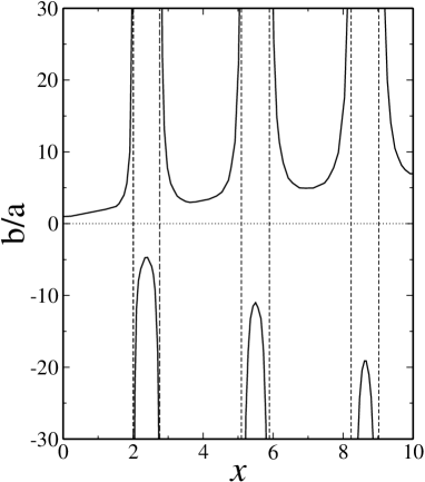
Figure 1: The ratio $b/a$ versus $x=r_{c}^{2}/(2r_{0}^{2})$ for the pairwise interaction kernel (32), $r_{c}=(m\gamma C/\hbar^{2})^{1/4}.$

As it is seen from Eq. (35), in the limit $x\to 0$ we get the hard-sphere result $b/a=1$ (see Fig. 1). The quantity $b$ (remind that $b$ is always positive!) is finite at $x=x^{(i)}_{0}$, while $b\to+\infty$ for $x\to x^{(i)}_{\infty}$. In the latter situation $b$ goes to infinity in such a way that $b/|a|\to+\infty$ though $|a|\to\infty$ for $x\to x^{(i)}_{\infty}$, too. Hence, $x^{(i)}_{0}$ and $x^{(i)}_{\infty}$ are both singular points of $b/a$. Let us stress that the zeros of the scattering length in the case considered have nothing to do with the weak-coupling regime for which, remind, $b/|a|\ll 1$. Operating with the kernel (32) we are not able to reach the weak-coupling regime at all because in this kernel is not bound from above. Now let us consider the situation of a negative scattering length being of special interest in the experimental context. The scattering length given by Eq. (33) is negative provided that $x^{(i)}_{0}<x<x^{(i)}_{\infty}$. As it seen from Fig. (1), for any of these intervals the ratio $b/a$ has a maximum value $[b/a]^{(i)}_{\rm max}$, and it decreases while $i$ increases. In particular, $[b/a]^{(1)}_{\rm max}\approx-5$, whereas $[b/a]^{(2)}_{\rm max}\approx-12$ and $[b/a]^{(3)}_{\rm max}\approx-18$ (see Fig. (1)). Hence, Eq. (35) turned out to make it possible to get some information about $b/a$ even without specifying the range of the relevant values of $x$ (in spite of the fact that this range is in principle known). Indeed, according to the mentioned above, the ratio $b/a$ does not exceed $[b/a]^{(1)}_{\rm max}\approx-5$ if the scattering length is negative. This suggests that the contribution of the pairwise potential to the kinetic energy is much larger than the absolute value of the corresponding contribution to the mean energy for a normal-state dilute Fermi gas with a negative scattering length at temperatures close enough to zero! The interaction energy is negative in this case and also much larger, if taken in absolute value, than the sum of the $a-$dependent terms in the Huang-Yang result. Note that for alkali atoms ties one can expect that $x\sim 10$, which means that $b/|a|\gtrsim 20$ (see Fig. 1). In view of the recent results ohara on a trapped Fermi gas, it is also of interest to consider behaviour of $b/a$ in vicinities of the special points $x^{(i)}_{\infty}$ and $x^{(i)}_{0}$. Varying the magnetic field acting on the system of ${}^{6}Li-$atoms, the authors of the paper ohara were interested in the regime of the Feshbach resonance, for which $a\to\infty$, and in the situation when $a\to 0$, as well. The both variants, as it follows from our consideration, are characterized by $b/|a|\gg 1$. Note that passage to the limit $a\to\infty$ in Eqs. (17) and (18) is not correct because it violates the expansion condition $k_{F}|a|\ll 1$. On the contrary, one can set $a=0$ in these equation, which leads to the exact result, beyond the perturbation theory,

$$\varepsilon_{\rm kin}\bigl{(}a\to 0\bigr{)}=\frac{3\hbar^{2}k_{F}^{2}}{10m}+\frac{\hbar^{2}k_{F}^{3}b}{3\pi m},$$ (36)

$$\varepsilon_{\rm int}\bigl{(}a\to 0\bigr{)}=-\frac{\hbar^{2}k_{F}^{3}b}{3\pi m}.$$ (37)

Equations (36) and (37) correspond to an unusual and extreme situation that, nevertheless, is experimentally attainable now (see Ref. bourdel ; ohara ). The total energy of the system is here equal (or practically equal) to that of an ideal Fermi gas, while the interaction and kinetic energies taken separately have nothing to do with those of a gas of noninteracting fermions. The most interesting particular case concerns the regime $k_{F}b\gg 1$, where the first term in Eq. (36) is negligible as compared to the second one. In this case $|\varepsilon_{\rm int}|\approx\varepsilon_{\rm kin}\propto n$.

Thus, the examples listed above show that in physically relevant situations the correct results for the kinetic and interaction energies of a dilute Fermi gas given by Eqs. (17) and (18) differ significantly (more than by order of magnitude!) from the pseudopotential predictions (24) and (25). As it is seen, in a Fermi gas the pairwise interaction has a profound effect on the kinetic energy contrary to a classical imperfect gas. And this well meets the conclusion on an interacting Bose gas derived in Refs. shanA ; shanB . A physically sound way of explaining this feature of quantum gases is to invoke the formalism of the in-medium pair wave functions. This is why below, in Sections (IV) and (V), the interaction and kinetic energies of a Fermi gas are investigated through the prism of this formalism.

IV Interaction energy via the pair wave functions

The derivation of the kinetic and interaction energies of a dilute ground-state Fermi gas given in Section II is mathematically adequate. However, from the physical point of view it has an obvious disadvantage. Namely, the microscopic information remains hidden in Eqs. (5), (17) and (18) due to its implicit usage in Section II. To eliminate this shortcoming, $\varepsilon_{\rm int}$ and $\varepsilon_{\rm kin}$ are considered below with a physically sound approach based on the in-medium pair wave functions (PWF).

For the sake of convenience, let us begin with the interaction energy. It is well-known that all the microscopic information concerning the $N-$particle system is contained in the $N-$particle density matrix. In the case of interest the $N-$matrix is defined by

$$\varrho_{N}(x_{1}^{\prime},x_{2}^{\prime} ,\dots,x_{N}^{\prime};x_{1},x_{2},\dots,x_{N})=$$

$$= \Psi^{*}(x_{1},x_{2},\dots,x_{N})\Psi(x_{1}^{\prime},x_{2}^{\prime},\dots,x_{N}^{\prime}),$$ (38)

where $\Psi(x_{1},x_{2},\dots,x_{N})$ is the ground-state normalized wave function, $\;x=\{{\bf r},\sigma\}$ stands for the space coordinates ${\bf r}$ and the spin $z-$projection $\sigma=\pm 1/2$. It is also known that actually we does not need to know the $N-$matrix in detail. In particular, to investigate the total system energy together with the kinetic and interaction ones, we can deal with the $2-$matrix defined by

$$\varrho_{2}(x_{1}^{\prime},x_{2}^{\prime};x_{1},x_{2})\!=\!\int\limits_{V}\! dx_{3}\!\dots\!dx_{N}\Psi^{*}(x_{1},x_{2},x_{3},\dots,x_{N})$$ (39)

$$\times\;\Psi(x_{1}^{\prime},x_{2}^{\prime},x_{3},\dots,x_{N}),$$

where in general

$$\int\limits_{V}\dots dx=\sum\limits_{\sigma}\int\limits_{V}\dots d^{3}r.$$

Let us introduce the eigenfuctions of the $2-$matrix $\xi_{\nu}(x_{1},x_{2})$ given by

$$\int\limits_{V}\!dx_{1}dx_{2}\;\varrho_{2}(x_{1}^{\prime},x_{2}^{\prime};x_{1},x_{2})\xi_{\nu} (x_{1},x_{2})=$$

$$= w_{\nu}\xi_{\nu}(x_{1}^{\prime},x_{2}^{\prime}),$$ (40)

where $w_{\nu}$ stands for the $\nu-$state eigenvalue. These eigenfuctions are usually called in-medium PWF bog . The $2$-matrix can be expressed in terms of its eigenfunctions and eigenvalues as follows:

$$\varrho_{2}(x_{1},x_{2};x_{1}^{\prime},x_{2}^{\prime})=\sum\limits_{\nu}w_{\nu}\;\xi^{*}_{\nu}(x_{1},x_{2})\xi_{\nu}(x_{1}^{\prime},x_{2}^{\prime}),$$ (41)

where it is implied that

$$\int\limits_{V}\!dx_{1}dx_{2}\;\xi^{*}_{\nu}(x_{1},x_{2})\xi_{\nu^{\prime}}(x_{1},x_{2})=\delta_{\nu\nu^{\prime}}.$$

From Eq. (39) it follows that

$$\int\limits_{V}\!dx_{1}dx_{2}\;\varrho_{2}(x_{1},x_{2};x_{1},x_{2})=1,$$ (42)

and, hence,

$$\sum_{\nu}w_{\nu}=1,$$ (43)

which allows one to interprete the eigenvalue $w_{\nu}$ as the probability of observing a particle pair in the $\nu-$state.

Now let us remind that the total momentum of the system of interest, the total system spin and its $z-$projection are conserved quantities note2 . This means that they commute with the $N-$particle density matrix because the latter is permutable with the system Hamiltonian. As the total pair momentum $\hbar{\rm\hat{Q}}$, the total pair spin $\hat{S}$ and its ${\rm Z}-$component $\hat{S}_{Z}$ commute with the total system momentum, total system spin and its ${\rm Z}-$projection, correspondingly, they commute with the $N-$matrix, too. If so, then one can derive that ${\rm\hat{Q}}$, $\hat{S}$ and $\hat{S}_{Z}$ are permutable with the $2-$matrix. This is why we can choose the eigenfunctions of the $2-$matrix in such a way that bog $\nu=\{\lambda,{\bf Q},S,m_{S}\}$, where $m_{S}$ is an eigenvalue of $S_{Z}$ and $\lambda$ stands for other quantum numbers. Hence, in the homogeneous situation one arrives at (see Refs. bog and shanC )

$$\xi_{\nu}(x_{1},x_{2})=\vartheta_{\nu}({\bf r},\sigma_{1},\sigma_{2})\,\exp\left(i{\bf Q}{\bf R}\right)/\sqrt{V},$$ (44)

where ${\bf r}={\bf r}_{1}-{\bf r}_{2}$ and ${\bf R}=({\bf r}_{1}+{\bf r}_{2})/2.$ As the in-medium bound pair states like the BCS-pairs are beyond the scope of the present publication, here we deal only with the scattering states. In other words, only the sector of the “dissociated” pair states is taken into consideration. Hence, $\nu=\{{\bf q},{\bf Q},S,m_{S}\}$, where ${\bf q}$ stands for the relative wave vector. This is why it is convenient to set by definition

$$\vartheta_{\nu}({\bf r},\sigma_{1},\sigma_{2})=\varphi_{\nu}({\bf r},\sigma_{1},\sigma_{2})/\sqrt{V}.$$ (45)

The pair interaction of interest does not depend on the spin variables, which means that $\varphi_{\nu}({\bf r},\sigma_{1},\sigma_{2})$ is expressed as

$$\varphi_{\nu}({\bf r},\sigma_{1},\sigma_{2})=\varphi_{\;{\bf q},{\bf Q},S}({\bf r})\,\chi_{S,m_{S}}\!(\sigma_{1},\sigma_{2}),$$ (46)

where for the singlet states $(S=0)$ one gets

$$\chi_{0,0}\!(\sigma_{1},\sigma_{2})=\Delta(\sigma_{1}+\sigma_{2})\mbox{sign}(\sigma_{1})/\sqrt{2},$$ (47)

while for the triplet wave functions $(S=1)$

$$\chi_{1,m_{S}} (\sigma_{1},\sigma_{2})=$$ (51)

$$=\left\{\begin{array}[]{ll}\Theta(-\sigma_{1})\Theta(-s_{2})&{\rm if}\quad m_{S}=-1,\\[2.84526pt] \Delta(\sigma_{1}+\sigma_{2})/\sqrt{2}&{\rm if}\quad m_{S}=\,\;\;0,\\[4.2679pt] \Theta(\sigma_{1})\Theta(\sigma_{2})&{\rm if}\quad m_{S}=\,\;\;1.\end{array}\right.$$

In Eqs. (47) and (51)

$$\Delta(\sigma)=\left\{\begin{array}[]{ll}0&{\rm if}\;\;\;\sigma\not=0,\\ 1&{\rm if}\;\;\;\sigma=0,\end{array}\right.\quad\Theta(\sigma)=\left\{\begin{array}[]{ll}1&{\rm if}\;\;\;\sigma\geq 0,\\ 0&{\rm if}\;\;\;\sigma<0.\end{array}\right.$$

Now, from Eq. (47) it follows that

$$\chi_{0,0}(\sigma_{1},\sigma_{2})=-\chi_{0,0}(\sigma_{2},\sigma_{1}).$$ (52)

Then, the Fermi statistics dictates

$$\varphi_{{\bf q},{\bf Q},0}({\bf r})=\varphi_{{\bf q},{\bf Q},0}({-\bf r})=\varphi_{-{\bf q},{\bf Q},0}({\bf r}),$$ (53)

and for $r\to\infty$ the wave function $\varphi_{{\bf q},{\bf Q},0}({\bf r})$ obeys the asymptotic regime

$$\varphi_{{\bf q},{\bf Q},0}({\bf r})\to\sqrt{2}\cos({\bf q}{\bf r}).$$ (54)

In turn, for triplet states Eq. (51) yields

$$\chi_{1,m_{S}}(\sigma_{1},\sigma_{2})=\chi_{1,m_{S}}(\sigma_{2},\sigma_{1}),$$ (55)

which leads to

$$\varphi_{{\bf q},{\bf Q},1}({\bf r})=-\varphi_{{\bf q},{\bf Q},1}({-\bf r})=-\varphi_{-{\bf q},{\bf Q},1}({\bf r}).$$ (56)

Now, another boundary regime

$$\varphi_{{\bf q},{\bf Q},1}({\bf r})\to\sqrt{2}\sin({\bf q}{\bf r}).$$ (57)

is fulfilled when $r\to\infty$.

Working in the thermodynamic limit $N\to\infty,V\to\infty,N/V=n=const$, it is more convenient to leave the $2-$matrix in favour of the so-called pair correlation function

$$F_{2}(x_{1},x_{2};x_{1}^{\prime},x_{2}^{\prime})=\bigl{\langle}\hat{\psi}^{\dagger}(x_{1})\hat{\psi}^{\dagger}(x_{2})\hat{\psi}(x_{2}^{\prime})\hat{\psi}(x_{1}^{\prime})\bigr{\rangle},$$ (58)

where $\langle\hat{A}\rangle$ stands for the statistical average of the operator $\hat{A}$, and $\hat{\psi}^{\dagger}(x)$, $\hat{\psi}(x)$ denote the field Fermi operators. The pair correlation function differs from the $2-$matrix by the normalization factor (see Ref. bog ),

$$F_{2}(x_{1},x_{2};x_{1}^{\prime},x_{2}^{\prime})=N(N-1)\varrho_{2}(x_{1}^{\prime},x_{2}^{\prime};x_{1},x_{2}),$$ (59)

so that $F_{2}$ remains finite while $\varrho_{2}$ approaches zero in the thermodynamic limit. Indeed, when $V\to\infty,\,N\to\infty,\,N/V=n\to const$, Eqs. (41) and (59), taken in conjunction with Eqs. (44) and (45), yield

$$F_{2}(x_{1},x_{2};x_{1}^{\prime},x_{2}^{\prime})=$$

$$=\!\!\sum\limits_{S,m_{S}}\!\int\frac{d^{3}\!{\rm q}\,d^{3}\!{\rm Q}}{(2\pi)^{6}}\;\rho_{S,m_{S}}\!({\bf q},{\bf Q})\varphi^{*}_{{\bf q},{\bf Q},S}({\bf r})\varphi_{{\bf q},{\bf Q},S}({\bf r}^{\prime})$$

$$\times\;\chi^{*}_{S,m_{S}}\!(\sigma_{1},\sigma_{2})\chi_{S,m_{S}}\!(\sigma_{1}^{\prime},\sigma_{2}^{\prime})\exp\left\{i{\bf Q}({\bf R}^{\prime}\!-\!{\bf R})\right\},$$ (60)

where the momentum-distribution function

$$\rho_{S,m_{S}}\!({\bf q},{\bf Q})=\lim_{\;V,N\to\infty}\Bigl{\{}N(N-1)w_{{\bf q},{\bf Q},S,m_{S}}\Bigr{\}}$$ (61)

is finite because $w_{{\bf q},{\bf Q},S,m_{S}}\sim 1/V^{2}$ (this follows from Eq. (43) when $V\to\infty$). For $\rho_{S,m_{S}}\!({\bf q},{\bf Q})$ one gets the relation

$$\sum\limits_{S,m_{S}}\int\frac{d^{3}\!{\rm q}d^{3}\!{\rm Q}}{(2\pi)^{6}}\;\rho_{S,m_{S}}\!({\bf q},{\bf Q})=n^{2}$$ (62)

resulting from Eqs. (43) and (61).

All the necessary formulae are now discussed and displayed, and one can turn to calculations of the interaction energy. Using the well-known expression

$$E_{\rm int}=\frac{1}{2}\int dx_{1}dx_{2}V(|{\bf r}_{1}-{\bf r}_{2}|)F_{2}(x_{1},x_{2};x_{1},x_{2})$$ (63)

and keeping in mind Eq. (60), one gets the following important relation:

$$\varepsilon_{\rm int} = \frac{1}{2n}\!\int\!d^{3}r\;V(r)$$ (64)

$$\times \;\sum\limits_{S,m_{S}}\!\int\frac{d^{3}\!{\rm q}\,d^{3}\!{\rm Q}}{(2\pi)^{6}}\;\rho_{S,m_{S}}\!({\bf q},{\bf Q})\;|\varphi_{{\bf q},{\bf Q},S}({\bf r})|^{2},$$

provided the equality

$$\sum_{\sigma_{1},\sigma_{2}}\chi^{*}_{S,m_{S}}\!(\sigma_{1},\sigma_{2})\chi_{S,m_{S}}\!(\sigma_{1},\sigma_{2})=1$$

is taken into account. Equation (64) directly connects the interaction energy per fermion with PWF and, thus, with the scattering waves defined by

$$\psi_{{\bf q},{\bf Q},0}({\bf r})=\varphi_{{\bf q},{\bf Q},0}({\bf r})-\sqrt{2}\cos({\bf q}{\bf r})$$ (65)

and

$$\psi_{{\bf q},{\bf Q},1}({\bf r})=\varphi_{{\bf q},{\bf Q},1}({\bf r})-\sqrt{2}\sin({\bf q}{\bf r}).$$ (66)

The scattering waves are immediately related to the pairwise-potential contribution to the spatial particle correlations. Setting $\psi_{{\bf q},{\bf Q},0}({\bf r})=\psi_{{\bf q},{\bf Q},1}({\bf r})=0$, or, in other words, ignoring that contribution and taking notice only of the correlations due to the statistics, one arrives at the Hartree-Fock scheme.

So far we did not invoke any approximation when operating with the $2-$matrix and pair correlation function note3 . However, taken in the regime of a dilute Fermi gas, Eq. (64) can significantly be simplified. Indeed, the lower densities, the lower momenta are typical of the system. This means that the pair momentum distibution $\rho_{S,m_{S}}({\bf q},{\bf Q})$ is getting more localized in a small vicinity of the point ${\rm q}={\rm q}=0$ when $n\to 0$. Consequently, the low-momentum approximation can be applied according to which for $n\to 0$ we get

$$\int\!\frac{d^{3}\!{\rm q}\,d^{3}\!{\rm Q}}{(2\pi)^{6}}\;\rho_{S,m_{S}}\!({\bf q},{\bf Q})\;|\varphi_{{\bf q},{\bf Q},S} ({\bf r})|^{2}\!\simeq$$

$$\simeq |\varphi_{S}({\bf r})|^{2}\;\eta_{\,S,m_{S}},$$ (67)

where

$$\eta_{\,S,m_{S}}\!=\!\!\int\!\frac{d^{3}\!{\rm q}\,d^{3}\!{\rm Q}}{(2\pi)^{6}}\;\rho_{S,m_{S}}({\bf q},{\bf Q})$$ (68)

and

$$\varphi_{S}({\bf r})=\lim\limits_{{\rm q,Q}\to 0}\varphi_{{\bf q},{\bf Q},S}({\bf r}).$$ (69)

From Eqs. (56) and (69) it follows that $\varphi_{S=1}({\bf r})=0$. This result, taken in conjunction with the low-momentum approximation of Eq. (67), makes it possible to conclude that Eq. (64) reduces for $n\to 0$ to

$$\varepsilon_{\rm int}\simeq\frac{\eta_{\,0,0}}{2n}\!\int\!d^{3}rV(r)|\varphi_{0}({\bf r})|^{2}.$$ (70)

The triplet states do not make any contribution to the interaction energy in the approximation (67), and this completely meets the usual expectations.

Now, to employ Eq. (70), one should have an idea concerning $\varphi_{0}({\bf r})$ and $\eta_{\,0,0}$. As to the limiting wave function $\varphi_{0}({\bf r})$, it can be determined by means of the following simple and custom arguments. In the dilution limit the pair wave function $\varphi_{{\bf q},{\bf Q},S}({\bf r})$ approaches the solution of the ordinary two-body Schrödinger equation

$$-(\hbar^{2}/m)\nabla^{2}\varphi_{{\bf q},{\bf Q},S}({\bf r}) +V(r)\varphi_{{\bf q},{\bf Q},S}({\bf r})=$$ (71)

$$=(\hbar^{2}q^{2}/m)\varphi_{{\bf q},{\bf Q},S}({\bf r})$$

with the boundary conditions given by Eqs. (53) and (56). Hence, in the limit $n\to 0$ the quantity $\varphi_{0}(r)$ has to obey the equation

$$-(\hbar^{2}/m)\nabla^{2}\varphi_{0}({\bf r})+V(r)\varphi_{0}({\bf r})=0,$$ (72)

where $\varphi_{0}({\bf r})\to\sqrt{2}$ when $r\to\infty$. Comparing Eq. (11) with Eq. (72), for $n\to 0$ one finds

$$\varphi_{0}({\bf r})=\sqrt{2}\,\varphi(r).$$ (73)

To complete calculation of the interaction energy, it only remains to find $\eta_{\,0,0}$. One can expect that when numbers of fermions with positive and negative spin $z-$projections are the same, the magnitude of $\rho_{S,m_{S}}({\bf q},{\bf Q})$ appears to be independent of the spin variables. In this case Eqs. (62) and (68) give

$$\eta_{S,m_{S}}=n^{2}/4.$$ (74)

Note that Eq. (74) can readily be found in a more rigorous way concerning the relation

$$\frac{1}{V^{2}}\int d^{3}r_{1}\,d^{3}r_{2}F_{2}(x_{1},x_{2};x_{1},x_{2})=n_{\sigma_{1}}n_{\sigma_{2}},$$ (75)

where $n_{\sigma}=\langle\hat{\psi}^{\dagger}(x_{1})\hat{\psi}(x_{1})\rangle$. This relation results from the definition of the pair correlation function (58). To derive Eq. (74) from Eq. (75), one should employ the latter in conjunction with Eqs. (47), (51) and (60) and, then, take account of $n_{\sigma}=\langle\hat{\psi}^{\dagger}(x_{1})\hat{\psi}(x_{1})\rangle=n/2$. Let us stress that Eq. (74) is not general. For example, when all the considered fermions have the spin $z-$projection equal to $+1/2$, one gets $\eta_{1,1}=n^{2}$ and $\eta_{0,0}=\eta_{1,-1}=\eta_{1,0}=0.$ As it is seen, in this case the interaction energy resulting from Eq. (70) is exactly amount to zero: one should go beyond the approximation defined by Eq. (67) to get an idea about $\varepsilon_{\rm int}$ of such a weekly interacting system. Here it is worth remarking that this week interaction is an obstacle that can prevent experimentalists from observing possible BCS-like pairing of fermions due to an extremely low temperature of the BCS-transition. To strengthen the interaction effects, it was, in particular, suggested stoof to complicate the experimental scheme in such a way that fermions with various spin $z-$projections would be trapped. In this case the low-momentum approximation yields a finite result for $\varepsilon_{\rm int}$. It is deductive to go in more detail concerning this situation because here another choice of the eigenfunctions of the $2-$matrix turned out to be convenient rather than that of Eq. (46). The details are in Appendix.

At last, inserting Eqs. (73) and (74) in Eq. (70) and making use of Eqs. (14) and (16), in the dilution limit one can derive $\varepsilon_{\rm int}\simeq\pi\hbar^{2}n(a-b)/m$, which is nothing else but the leading term in Eq. (18). Note that to derive the next-to-leading terms in the expression for the interaction energy via PWF, one should construct a more elaborated model similar to that of Refs. shanA ; shanB concerning a dilute Bose gas. The model like that has to take into account in-medium corrections to PWF to go beyond the approximation of Eq. (67). Though this investigation is beyond the scope of the present publication, there are some important remarks on the in-medium corrections to the eigenfunctions of the $2-$matrix in the next section.

Here it is of interest to check if Eq. (70) yields Eq. (25) when replacing $V(r)$ by the pseudopotential $V^{(\rm ps)}(r)$. The simplest way of escaping divergences while operating with the pseudopotential is to adopt $V^{(\rm ps)}(r)=(4\pi\hbar^{2}a/m)\delta({\bf r})$ in conjunction with the Hartree-Fock scheme. For example, exactly this way was used in the classical paper by Pitaevskii when deriving the well-known Gross-Pitaevskii equation for the order parameter of the Bose-Einstein condensation in a dilute Bose gas gp . A more elaborated variant, which goes beyond the Hartree-Fock framework, requires a more sophisticated choice of the pseudopotential which, for the particular case of the hard-sphere interaction, is of the form $V^{(\rm ps)}(r)=(4\pi\hbar^{2}a/m)\delta({\bf r})(\partial/\partial r)r$ hy . The aim of this variant is to calculate not only the total system energy but some additional important characteristics (for instance, the pair correlation function) which can not be properly considered in the former way. Complicating the pseudopotential construction allows one to escape a double account of some scattering channels (this fact is known since the Thesis by Noziéres). This double account appears due to the fact that the particle scattering makes contribution to the pseudopotential. In our case, of course, the simplest choice is enough. Now, replacing $V(r)$ by $V^{(\rm ps)}(r)=(4\pi\hbar^{2}a/m)\delta({\bf r})$ in Eq. (70) and setting $\psi(r)=0\;(\varphi(r)=1)$, for $n\to 0$ one derives $\varepsilon^{(\rm ps)}_{\rm int}\simeq(\pi\hbar^{2}a\,n/m)$. It is just the leading term in Eq. (25). This supports the conclusion that the pseudopotential is not able to produce correct results for the kinetic and interaction energies of dilute quantum gases.

Here let us make some remarks on the momentum distribution of the “dissociated” pairs $\rho_{S,m_{S}}({\bf q},{\bf Q})$. The calculational procedure leading to Eq. (70) does not involve a detailed knowledge of this distribution. However, it can be completely refined. In Ref. shanC it was suggested to derive $\rho_{S,m_{S}}({\bf q},{\bf Q})$ via the correlation-weakening principle (CWP). According to CWP the pair correlation function obeys the following relation:

$$F_{2}(x_{1},x_{2};x_{1}^{\prime},x_{2}^{\prime})\to F_{1}(x_{1};x_{1}^{\prime})\,F_{1}(x_{2};x_{2}^{\prime})$$ (76)

when

$$|{\bf r}_{1}-{\bf r}_{2}|\to\infty,\;|{\bf r}_{1}-{\bf r}_{1}^{\prime}|=const,\;|{\bf r}_{2}-{\bf r}_{2}^{\prime}|=const.$$

In Eq. (76) we set $F_{1}(x_{1};x_{1}^{\prime})=\langle\hat{\psi}^{\dagger}(x_{1})\hat{\psi}(x_{1}^{\prime})\rangle$. So, the pair momentum distribution $\rho_{S,m_{S}}({\bf q},{\bf Q})$, which appears in the expansion of $F_{2}$ in the set of its eigenfunctions, can be expressed in terms of the single-particle momentum distribution $n_{\sigma}(k)=\langle a^{\dagger}_{\sigma}({\bf k})a_{\sigma}({\bf k})\rangle$, that comes into the plane-wave expansion for $F_{1}$. In the case of interest, when the both distribution functions turn out to be independent of spin variables, this leads to

$$\rho_{S,m_{S}}({\bf q},{\bf Q})=n\bigl{(}|{\bf Q}/2+{\bf q}|\bigr{)}\,n\bigl{(}|{\bf Q}/2-{\bf q}|\bigr{)},$$ (77)

where, by definition, $n(k)=n_{\sigma}(k)$. Concluding let us set, for the sake of demonstration, $n(k)=1$ for $k\leq k_{F}$, $n(k)=0$ for $k>k_{F}$ and return to Eq. (67). Inserting Eq. (77) in the right-hand side of Eq. (67) and utilizing this single-particle momentum distribution of an ideal Fermi gas, we arrive at the left-hand side of Eq. (67) due to $k_{F}\to 0$ when $n\to 0$. This example is a good illustration of the idea of the low-momentum approximation introduced by Eq. (67).

Thus, in Section IV it is demonstrated how to calculate the interaction energy of a dilute Fermi gas from the first principles, beyond the formula by Huang and Yang taken in conjunction with the Hellmann-Feynman theorem. Though the results of this section make Eq. (18) physically sound and support the conclusion about strong influence of the pairwise interaction on the system kinetic energy, the nature of this influence is not highlighted yet. The detailed discussion of this nature is given in Section V.

V Kinetic energy via the pair wave functions

Some hints as to how to proceed with the problem of the influnce of the pairwise particle interaction on the kinetic energy can be found in the Bogoliubov model of a weakly interacting Bose gas and in the BCS-approach. As it shown in Refs. shanA ; shanB , there exists some important relation which mediates between the pairwise boson interaction and single-boson momentum distribution $n_{B}(k)$ in the Bogoliubov model. For the ground-state case this relation is the form

$$n_{B}(k)\bigl{[}1+n_{B}(k)\bigr{]}=n^{2}_{0}\psi_{B}^{2}(k),$$ (78)

where $\psi_{B}(k)$ is the Fourier transform of the scattering part of the bosonic PWF corresponding to ${\bf q}={\bf Q}=0$, and $n_{0}$ stands for the density of condensed bosons. When the pairwise boson interaction is “switched off”, there is no scattering. So, bosonic PWF are the symmetrized plane waves and $\psi_{B}(k)=0$. In this case Eq. (78) has the only physical solution $n_{B}(k)=0$, that corresponds to an ideal Bose gas with the zero condensate depletion and the zero kinetic energy. On the contrary, “switching on” the pairwise interaction leads to $\psi_{B}(k)\not=0$, and we arrive at the regime of a nonzero condensate depletion, when $n_{B}(k)\not=0$ and the kinetic energy is not equal to zero, as well.

A similar situation occurs in the BCS-model. There is again some corner-stone relation mediating between the pairwise interaction and the single-particle momentum distribution $n_{BCS}(k)$. It can be expressedshanC as

$$n_{BCS}(k)\bigl{[}1-n_{BCS}(k)\bigr{]}=n^{2}_{s}\,\psi_{BCS}^{2}(k),$$ (79)

where $\psi_{BCS}(k)$ is the Fourier transform of the internal wave function of a condensed bound pair of fermions, $n_{s}$ is the density of this pairs.“Switching off” the pairwise attraction leads to disappearnce of the bound pair states: $\psi_{BCS}(k)=0$. In this case there are two branches of the solution of Eq. (78): $n_{BCS}=1$ and $n_{BCS}=0$. Below the Fermi momentum the first branch is advantageous from the thermodynamic point of view, while the second one is of relevance above. So, one gets the regime of an ideal Fermi gas with the familiar kinetic energy, often called the Fermi energy. When “switching on” the attraction, some significant corrections to the momentum distribution of an ideal Fermi gas arise. This corrections are dependent of the mutual attraction of fermions and make a significant contribution to the kinetic energy additional to the Fermi energy.

Now, keeping in mind the examples listed above, one can suppose that the relation connecting PWF (strictly speaking, the scattering waves and bound waves) with the single-particle momentum distribution is some general feature of quantum many-body systems. If so, exactly this relation has to be responsible for the influence of the pairwise interaction on the kinetic energy of the quantum gases. For a ground-state dilute Fermi gas with no pairing effects the relation of interest can be constructed in the form

$$n(k)[1-n(k)]={\cal L}(k),$$ (80)

where ${\cal L}(k)$ stands for a functional of the in-medium scattering waves $\psi_{{\bf q},{\bf Q},S}({\bf r})$. To go in more detail concerning the functional ${\cal L}(k)$, we should try to calculate the kinetic energy, starting durectly from $n(k)$ of Eq. (80). This equation results in

$$n(k)=\left\{\begin{array}[]{ll}\bigl{[}1+\sqrt{1-4{\cal L}(k)}\bigr{]}/2&\;\;{\rm if}\quad k\leq{\cal K}_{F},\\[4.2679pt] \bigl{[}1-\sqrt{1-4{\cal L}(k)}\bigr{]}/2&\;\;{\rm if}\quad k>{\cal K}_{F},\end{array}\right.$$ (81)

where $\hbar{\cal K}_{F}$ stands for the Fermi momentum. In the present paper a weakly nonideal gas of fermions is under investigation note4 , which means that the single-fermion momentum distribution approaches the ideal-gas Fermi distribution in the dilution limit: ${\cal L}(k)\to 0$ and ${\cal K}_{F}\to k_{F}$ for $n\to 0$. Then, Eq. (81) can be rewritten for $n\to 0$ as

$$n(k)\simeq\bigl{[}1-\ell(k)\bigr{]}\Theta(k_{F}-k)+\ell(k)\Theta(k-k_{F}),$$ (82)

where the dilution expansions ${\cal L}(k)=\ell(k)(1+\ldots)$ and ${\cal K}_{F}=k_{F}(1+\ldots)$ are implied. Taken together with the familiar formula

$$E_{\rm kin}=V\sum_{\sigma}\int\frac{d^{3}k}{(2\pi)^{3}}\;T_{k}n_{\sigma}(k),$$ (83)

Eq. (82) leads for $n\to 0$ to

$$\varepsilon_{\rm kin}=\frac{3\hbar^{2}k^{2}_{F}}{10m}+\frac{2}{n}\int\frac{d^{3}k}{(2\pi)^{3}}T_{k}\,\ell(k)+\ldots.$$ (84)

Note that the characteristic length $b$ given by (16) can be rewritten as

$$b=\frac{m}{2\pi\hbar^{2}}\int\frac{d^{3}k}{(2\pi)^{3}}T_{k}\psi^{2}(k),$$

where $\psi(k)$ is the Fourier transform of the scattering wave $\psi(r)$ (see Eq. (12)). Keeping this in mind and comparing Eqs. (17) with (84), we can find for $n\to 0$ that

$$\ell(k)=(n^{2}/4)\psi^{2}(k).$$ (85)

Hence, the quantuty ${\cal L}(k)$ is indeed a functional of $\psi_{{\bf p},{\bf q},S}({\bf r})$ that reduces to the right-hand side of Eq. (85) in the limit $n\to 0$. So, our expectations about the relation mediating between the pairwise interaction and single-particle momentum distribution in a dilute Fermi gas turn out to be adequate. Let us remark that Eq. (82) is a good approximation only when calculating the dilution expansion for the kinetic energy (strictly speaking, the leading and next-to-leading terms). However, to go in more detail concerning the single-fermion momentum distribution, one should be based on Eq. (81) rather than on Eq. (82). Indeed, Eq. (11) can be rewritten as

$$\psi(k)=-\frac{1}{2T_{k}}\int d^{3}r\varphi(r)V(r)\exp(-i{\bf k}{\bf r}).$$

From Eq. (10) it follows that $\int d^{3}r\varphi(r)V(r)=4\pi\hbar^{2}a/m$. Therefore, $\psi(k)\propto-1/k^{2}$ when $k\to 0$. Taken in the first two orders of the dilution expansion, the kinetic energy is not affected by this singularity. However, $n(k)$ is rather sensitive to it. Actually in-medium corrections to $\psi(k)$ should be involved to find the adequate behaviour of $n(k)$ when $k\to\infty$. Indeed, low momenta correspond to large particle separations where influence of the surrounding medium on PWF can be of importance even in the dilution regime.

Discussion about the in-medium corrections to PWF can be illustrated as follows. Keeping in mind the replacement of $\varphi_{0}(r)$ by $\sqrt{2}\varphi(r)$ in Eq. (70), one can suggest to abandon the approximation ${\cal L}(k)\simeq(n^{2}/4)\psi^{2}(k)$ in favour of

$${\cal L}(k)\simeq(n^{2}/8)|\psi_{0}(k)|^{2},$$ (86)

where $\psi_{0}(k)$ is the Fourier transform of $\psi_{0}(r)=\varphi_{0}(r)-\sqrt{2}$. As $\psi_{0}(k)\to\sqrt{2}\psi(k)$ for $n\to 0$, the correct dilution limit ${\cal L}(k)\to\ell(k)$ results from Eq. (86). However, the advantage of Eq. (86) as compared with ${\cal L}(k)\simeq\ell(k)$ is that $\psi_{0}(k)$ is an in-medium PWF and, so, includes in-medium corrections at any finite particle density. This is why one can expect that Eq. (86), taken together with Eq. (81), gives adequate results for both the kinetic energy and the single-fermion momentum distribution. To be convinced of this, let us try first to have a guess about the in-medium corrections to PWF. Here it is natural to start from the expectation that the Fermi sphere is completely occupied when $n\to 0$. This means (see Eqs. (80) and (86)) that $\psi_{0}(k)=0$ at $k\leq{\cal K}_{F}\simeq k_{F}$. On the contrary, at large $k$ (small particle separations!) $\psi_{0}(k)$ can not be significantly affected by surroundings. So, $\psi_{0}(k)$ in this regime is nearly be governed by the ordinary two-body Schrödinger equation for the internal wave function of the interacting pair at ${\bf q}=0$. Combining these two regimes, one can approximately write

$$2T_{k}\psi_{0}(k)+\Theta(k\!-\!k_{F})\!\!\!\int\!\!d^{3}r\varphi_{0}(r)\!V(r)\!\exp(-i{\bf k}{\bf r})=0.$$ (87)

Stress that the jump in the Fourier transform of $\psi_{0}(r)$ at $k=k_{F}$ does not imply a jump of $\psi_{0}(r)$ itself. Passing to the coordinate representation, Eq. (87) gets the form

$$-\frac{\hbar^{2}}{m}\nabla^{2}\varphi_{0}(r)+ \varphi_{0}(r)V(r)=$$

$$= \int d^{3}r^{\prime}\varphi_{0}(r^{\prime})V(r^{\prime})G({\bf r}-{\bf r}^{\prime}),$$ (88)

where $G({\bf r})=\int_{k<k_{F}}d^{3}k/(2\pi)^{3}\exp[i{\bf k}{\bf r}]$. Equation (88) is nothing else but the simplest version of the Bethe-Goldstone equation bg for the internal wave function of the interacting pair at ${\bf Q}={\bf q}=0$. So, the “veto” upon appearance of intermediate scattering states inside the Fermi sphere (see the page 320 in the textbook fw ), that allows for passing from the ordinary two-body Schrödinger equation to the Bethe-Goldstone one, can be easily explained beyond any intuitive arguments with the help of the relation connecting the scattering parts of the in-medium PWF with the single-particle momentum distribution.

Now, after the glance at the problem of medium influence on PWF, we can try to outline a more elaborated way of treating the in-medium pair wave functions. Indeed, it turns out that there are everything at our disposal to derive some two coupled equations which make it possible to find $\psi_{0}(k)$ in conjunction with $n(k)$. The first of these equations connecting $\psi_{0}(k)$ with $n(k)$ results from Eqs. (81) and (86). As to the second equation, some longer but straightforward calculations are needed. The point is that Eqs. (70) and (83) enable representation of the total system energy as a functional of $\varphi_{0}(r)$ and $n(k)$. Hence, we are able to derive the second equation from the minimum condition for this functional. Making variation with respect to $\psi^{*}_{0}(r)$ and $n(k)$, one gets

$$\frac{\delta E}{V}=\int\frac{d^{3}k}{(2\pi)^{3}} \Bigl{[}2T_{k}\delta n(k)+\frac{n^{2}}{8}\delta\psi^{*}_{0}(k)$$ (89)

$$\times\int d^{3}r\varphi_{0}(r)V(r)\exp(-i{\bf k}{\bf r})\Bigr{]}.$$

To extract the second equation from Eq. (89), one should keep in mind that the infinitesimal changes $\delta n(k)$ and $\delta\psi^{*}_{0}(k)$ are not independent due to the first equation. They are related to one another by

$$[1-2n(k)]\delta n(k)=(n^{2}/8)\psi_{0}(k)\delta\psi^{*}_{0}(k).$$ (90)

In addition, a change of $n(k)$ should not affect the total number of fermions $N=2\int d^{3}k/(2\pi)^{3}n(k)$. So, the equation of interest has the form

$$\delta(E-\mu N)=0,$$ (91)

where $\mu$ stands for the chemical potential. A combination of Eqs. (89), (90) and (91) yields

$$\psi_{0}(k)=\frac{1-2n(k)}{2(\mu-T_{k})}\int d^{3}r\varphi_{0}(r)V(r)\exp(-i{\bf k}{\bf r}).$$ (92)

Equation (92) is more complicated but very similar to Eq. (87). This is especially clear in the light of the fact that for $n\to 0$ one gets $n(k)\to\Theta(k_{F}-k)$. As it is seen, when $k\to\infty$, Eq. (92) is reduced to the ordinary Schrödinger equation for the internal wave function of an interacting pair with ${\bf q}=0$. While in the opposite regime, for $k\to 0$, Eq. (92) acquires completely different form with significant contribution of medium-dependent terms. So, in-medium corrections are indeed of importance for getting an adequate behaviour of $n(k)$ and $\psi_{0}(k)$ at small absolute values of the wave vector ${\bf k}$. It is worth noting that the equation derived by Galitskii gal for the scattering part of his “effective wave function of two particles in medium”(see Eq. (11.39) in Ref. fw ) exactly reduces to Eq. (92) in the case when the center-of-mass and relative wave vectors are equal to zero. The author of Ref. gal introduced the name “effective wave function” only due to similarity of the equation for that quantity to the Schrödinger equation for two particles in free space. To the best knowledge of the present authors, Galitskii did not associate those effective wave functions with the eigenfunctions of the $2-$matrix. However, the derived result strongly suggests that they are actually the eigenfunctions of the reduced density matrix of the second order. If so, there is a promising possibility of using the Galitskii equation in combination with the $2-$matrix, which can produce correct results for $\varepsilon$ and aslo for $\varepsilon_{\rm kin}$ and $\varepsilon_{\rm int}$. Note that in the case of a dilute Bose gas the pseudopotential approach does not yield correct picture of the short-range boson correlations in addition to the failure with the kinetic and interaction energies shanA . This is why one can expect the same fault with the pseudopotential in the Fermi case. In view of this fact, it is worth displaying one more advantage of the formalism of PWF. It produces the correct picture of the short-range spatial correlations. Indeed, from Eq. (60) it follows that the pair distribution function $g(r)$, defined by $g(r)=(1/n^{2})\sum_{\sigma_{1},\sigma_{2}}\!\!F_{2}(x_{1},x_{2};x_{1},x_{2})$, can be expressed as

$$g(r)=\frac{1}{n^{2}}\!\!\int\!\frac{d^{3}\!{\rm q}\,d^{3}\!{\rm Q}}{(2\pi)^{6}}\;\rho_{S,m_{S}}\!({\bf q},{\bf Q})\;|\varphi_{{\bf q},{\bf Q},S}({\bf r})|^{2}.$$ (93)

When using the low-momentum approximation together with Eqs. (73) and (74), one gets that for $r\ll 1/k_{F}$ and $n\to 0$ Eq. (93) reads

$$g(r)\simeq(1/2)\varphi^{2}(r).$$ (94)

This result differs from the pair distribution function of a dilute Bose gas shanA ; shanB by the factor $1/2$ appearing precisely due to the Fermi statistics. Note that this factor manifests itself in the total system energy, too. Indeed, it is well-known that the leading term in the dilution expansion for the total energy of a ground-state uniform Bose gas is twice more than the first $a-$dependent term in the corresponding expansion for a Fermi gas. Thus, contrary to the pseudopotential calculations for a Bose gas (see Ref. shanA ), there is no negative values of $g(r)$ at small particle separations when using the formalism of the $2-$matrix. At last, we remark that it would be also of importance to work out some arguments which would make it possible to refine the form of ${\cal L}(k)$, say, the “imperfection” functional. This is of interest in view of moving beyond the dilution regime in the investigations of the quantum many-body systems.

VI Conclusion and comments

Concluding, let us highlight the most important points of this article.

First, the low-density expansions for the kinetic and interaction energies of a uniform ground-state Fermi gas with a repulsive pairwise interaction have been calculated up to the third order in the dilution parameter $k_{F}a$. These quantities turn out to depend on the interparticle potential trough the two characteristic lengths $a$ and $b$ given by Eqs. (10) and (16). In the first orders the $b-$dependent terms are cancelled in the sum of $E_{\rm kin}+E_{\rm int}$, and, so, the total energy $E$, if taken in those orders, involves only the scattering length $a$, as it is well-known. However, all the higher orders of the dilution expansion for $E$ are expected to emonstrate $b-$dependence.

Second, the calculations have been fulfilled in two ways with the aim of controlling our conclusions and making the present investigation more physically sound. One of those ways is based on the Hellmann-Feynman theorem which is utilized in conjunction with the useful variational theorem for the scattering length when deriving $E_{\rm kin}$ and $E_{\rm int}$ from the familiar result by Huang and Yang for the total energy of a ground-state dilute uniform Fermi gas. Another way invokes a formalism of the in-medium pair wave functions. This variant allows one to find $E_{\rm kin}$ and $E_{\rm int}$ starting directly from the first principles. The advantage of the latter way is that it makes the underline physics more clear and enables to go in more detail concerning the spatial fermion correlations and their influence on the quantities of interest.

Third, the ratio of the two characteristic lengths $b/a$ has been investigated for the model pairwise interaction often used in the context of the alkali-metal atoms. In particular, according to the found results, one faces a rather interacting gas of fermions in the situation when $a=0$. The matter is that the sum of the terms coming from the pairwise interaction is here exactly cancelled in the total energy but, nevertheless, they make significant contributions to $E_{\rm kin}$ and $E_{\rm int}$, taken separately. This is a consequence of presence of the two characteristic lengths: when $a$ is amount to zero, then $b$ can take any positive value depending on a particular form of a pairwise interaction. Moreover, $b$ can be extremely large in such an “uninteracting” gas. Thus, one should be very careful with an experimantal analysis of a spatial expansion of a trapped gases with $a=0$ (see Ref. bourdel ; ohara ). Actually in such situations the interaction energy can be extremely large in absolute value and has the negative sign.

Forth, important arguments have been presented that any many-particle quantum system is characterized by some cornerstone relation connecting the single-particle momentum distribution with the in-medium pair wave functions. Exactly it is responsible for influence of the pairwise interaction on the kinetic energy of quantum gases. The form of this relation for a repulsive ground-state uniform Fermi gas has been established in the leading-order in the dilution parameter $k_{F}a$. It is worth noting that if incorporated in the formalism of the $2-$matrix, the relation under question allows for getting Schrödinger-like equations for the in-medium pair wave functions. The simplest variant of these equations reduces to the Bethe-Goldstone one. More elaborated version demonstrates important and deep parallels with the Galitskii consideration. Thus, one can expect that the failure of the pseudopotential approach with $E_{\rm kin}$ and $E_{\rm int}$ and, also, with the spatial particle correlations occurs somewhere during its second step when the effective interaction extracted from the Galitskii equation is inserted in the weak-coupling expansions for the physical quantities.

This work was supported by the RFBR grant 00-02-17181. The author thanks A.Yu. Cherny for the helpful discussions.

Appendix A

In the appendix the situation of a dilute gas of fermions with the single-particle spin $\ell/2$ ($\ell>1$ is some integer parameter) is under investigation. Let particles with some two $z-$projections of single-particle spin be present, for example, $\ell/2$ and $\ell/2-\ell^{\prime}$, where $\ell^{\prime}$ is integer and $\ell^{\prime}\leq\ell$. And let the density of the fermions with the projection $\ell/2$ is $n_{\ell/2}$, whereas $n_{\ell/2-\ell^{\prime}}$ corresponds to $\ell/2-\ell^{\prime}$. This situation is of special interest in view of the proposal of Ref. stoof where a spin pattern like this was suggested to strengthen the pairwise-interaction effects in a magnetically trapped vapour of ${}^{6}Li-$fermions. In the case under consideration it turned out to be more convenient to compose a set of the eigenfunctions for the $2-$matrix in a way slightly different with respect to that of Section IV. The difference is that we now adopt $\nu=\{{\bf q},{\bf Q},S_{Z},\delta_{S_{Z}}\}$, where $S_{Z}$ stands for eigenvalues of $\hat{S_{Z}}$, the $Z-$projection of the total pair spin, while $\delta_{S_{Z}}$ does not correspond to some important physical characteristics but simply enumerates degenerate states (for more detail, see formulae below). So, here we do not care about the total pair spin, in order to simplify all calculations. This choice is quite under the general rules of the quantum mechanics together with that of Section IV (see the discussion concerning the eigenstates of the $2-$matrix in this section). Equation (46) in the situation of interest is of the form

$$\varphi_{\nu}({\bf r},\sigma_{1},\sigma_{2})=\varphi^{(\delta)}_{{\bf q},{\bf Q}}({\bf r})\,\chi^{(\delta)}_{S_{Z}}\!(\sigma_{1},\sigma_{2}),$$ (95)

where the spin variable $\sigma_{i}\;(i=1,2)$ takes the values $\ell/2$ and $\ell/2-\ell^{\prime}$. In Eq. (95) the condensed notation $\delta=\delta_{S_{Z}}$ is introduced, and $\delta$ is taken as a superscript to stress the fact that $\delta$ is here some auxiliary quantity rather than an important physical characteristics. The eigenstates for $\hat{S}_{Z}$ are now chosen as follows:

$$\bigl{|}\chi^{(\delta=1)}_{S_{Z}=\ell}\bigr{\rangle}=\bigl{|}\frac{\ell}{2}\bigr{\rangle}\bigl{|}\frac{\ell}{2}\bigr{\rangle},$$

$$\bigl{|}\chi^{(\delta=1)}_{S_{Z}=\ell-\ell^{\prime}}\bigr{\rangle}=\frac{1}{\sqrt{2}}\biggl{(}\bigl{|}\frac{\ell}{2}\bigr{\rangle}\bigl{|}\frac{\ell}{2}-\ell^{\prime}\bigr{\rangle}+\bigl{|}\frac{\ell}{2}-\ell^{\prime}\bigr{\rangle}\bigl{|}\frac{\ell}{2}\bigr{\rangle}\biggr{)},$$

$$\bigl{|}\chi^{(\delta=2)}_{S_{Z}=\ell-\ell^{\prime}}\bigr{\rangle}=\frac{1}{\sqrt{2}}\biggl{(}\bigl{|}\frac{\ell}{2}\bigr{\rangle}\bigl{|}\frac{\ell}{2}-\ell^{\prime}\bigr{\rangle}-\bigl{|}\frac{\ell}{2}-\ell^{\prime}\bigr{\rangle}\bigl{|}\frac{\ell}{2}\bigr{\rangle}\biggr{)},$$

$$\bigl{|}\chi^{(\delta=1)}_{S_{Z}=\ell-2\ell^{\prime}}\bigr{\rangle}=\bigl{|}\frac{\ell}{2}-\ell^{\prime}\bigr{\rangle}\bigl{|}\frac{\ell}{2}-\ell^{\prime}\bigr{\rangle}.$$ (96)

As it is seen, there is no degeneracy for $S_{Z}=\ell$ and $S_{Z}=\ell-2\ell^{\prime}$ when the only variant $\delta_{S_{Z}}=1$ is involved. While for $S_{Z}=\ell-\ell^{\prime}$ two possible eigenstates of $\hat{S}_{Z}$ are present: $\delta_{\ell-\ell^{\prime}}=1,2$. From Eq. (96) it follows that

$$\chi^{(1)}_{S_{Z}}(\sigma_{1},\sigma_{2})=\chi^{(1)}_{S_{Z}}(\sigma_{2},\sigma_{1}),$$ (97)

and, due to the Fermi statistics, we find

$$\varphi^{(1)}_{{\bf q},{\bf Q}}({\bf r})=-\varphi^{(1)}_{{\bf q},{\bf Q}}(-{\bf r})=-\varphi^{(1)}_{-{\bf q},{\bf Q}}({\bf r}),$$ (98)

the wave function $\varphi^{(1)}_{{\bf q},{\bf Q}}({\bf r})$ approaching $\sqrt{2}\sin({\bf q}{\bf r})$ when $r\to\infty$. On the contrary, for $\delta=2$ one gets

$$\chi^{(2)}_{S_{Z}}(\sigma_{1},\sigma_{2})=-\chi^{(2)}_{S_{Z}}(\sigma_{2},\sigma_{1}),$$ (99)

which results in

$$\varphi^{(2)}_{{\bf q},{\bf Q}}({\bf r})=\varphi^{(2)}_{{\bf q},{\bf Q}}(-{\bf r})=\varphi^{(2)}_{-{\bf q},{\bf Q}}({\bf r}),$$ (100)

where $\varphi^{(2)}_{{\bf q},{\bf Q}}({\bf r})$ tends to $\sqrt{2}\cos({\bf q}{\bf r})$ for $r\to\infty$.

Now, one has everything at his disposal, to express the pair correlation function $F_{2}$and interaction energy $E_{\rm int}$ in terms of PWF. Taken in conjunction with Eqs. (41), (44) and (45), Eq. (95) in the thermodynamic limit yields

$$F_{2}(x_{1},x_{2};x_{1},x_{2})= \!\!\!\sum\limits_{S_{Z},\delta}\int\frac{d^{3}\!{\rm q}\,d^{3}\!{\rm Q}}{(2\pi)^{6}}\rho^{(\delta)}_{S_{Z}}\!({\bf q},{\bf Q})$$ (101)

$$\times \;|\varphi^{(\delta)}_{{\bf q},{\bf Q}}({\bf r})|^{2}\;|\chi^{(\delta)}_{S_{Z}}\!(\sigma_{1},\sigma_{2})|^{2}.$$

Further, inserting Eq. (101) in Eq. (63) and keeping in mind

$$\sum_{\sigma_{1},\sigma_{2}}|\chi^{(\delta)}_{S_{Z}}\!(\sigma_{1},\sigma_{2})|^{2}=1,$$

one can arrive at

$$E_{\rm int}/V = \frac{1}{2}\!\int\!d^{3}r\;V(r)$$ (102)

$$\times \!\sum\limits_{S_{Z},\delta}\int\!\frac{d^{3}\!{\rm q}\,d^{3}\!{\rm Q}}{(2\pi)^{6}}\;\rho^{(\delta)}_{S_{Z}}\!({\bf q},{\bf Q})\;|\varphi^{(\delta)}_{{\bf q},{\bf Q}}({\bf r})|^{2}.$$

The low-momentum approximation (for more detail, see Eq. (67)) makes it possible to extremely simplify this expression if the dilution limit is of interest. So, for $n_{\ell/2},n_{\ell/2-\ell^{\prime}}\to 0$ one gets

$$E_{\rm int}/V\simeq\frac{\eta^{(2)}_{\ell-\ell^{\prime}}}{2}\int d^{3}rV(r)|\varphi^{(2)}({\bf r})|^{2},$$ (103)

where

$$\eta^{(\delta)}_{S_{Z}}\!=\!\!\int\!\frac{d^{3}\!{\rm q}\,d^{3}\!{\rm Q}}{(2\pi)^{6}}\;\rho^{(\delta)}_{S_{Z}}({\bf q},{\bf Q})$$ (104)

and

$$\varphi^{(\delta)}({\bf r})=\lim\limits_{{\rm q,Q}\to 0}\varphi^{(\delta)}_{{\bf q},{\bf Q}}({\bf r}).$$ (105)

Only the terms corresponding to $\delta=2$ make contribution to the interaction energy (103) in the dilution limit because $\varphi^{(1)}({\bf r})$ is exactly equal to zero as it is seen from Eqs. (98) and (105). Following the arguments of Section IV (see the discussion just after Eq. (70)) one can rewrite Eq. (103) in the form

$$E_{\rm int}/V\simeq\eta^{(2)}_{\ell-\ell^{\prime}}\int d^{3}rV(r)\varphi^{2}(r)$$ (106)

with $\varphi(r)$ obeying Eq. (11).

To have an idea about $\eta^{(2)}_{\ell-\ell^{\prime}}$, let us turn to Eq. (75). Inserting Eq. (101) in Eq. (75), one can find

$$\sum\limits_{S_{Z},\delta}\int\frac{d^{3}\!{\rm q}\,d^{3}\!{\rm Q}}{(2\pi)^{6}}\rho^{(\delta)}_{S_{Z}}\!({\bf q},{\bf Q})\,|\chi^{(\delta)}_{S_{Z}}\!(\sigma_{1},\sigma_{2})|^{2}=n_{\sigma_{1}}n_{\sigma_{2}}$$ (107)

provided that the necessary normalization condition $(1/V)\int_{V}d^{3}r|\varphi^{(\delta)}_{{\bf q},{\bf Q}}({\bf r})|^{2}=1$ is taken into account (see Eqs. (45) and (95)). From Eqs. (96) and (107) it follows that

$$\frac{1}{2}\int\frac{d^{3}\!{\rm q}\,d^{3}\!{\rm Q}}{(2\pi)^{6}}\Bigl{[}\rho^{(1)}_{\ell-\ell^{\prime}}\!({\bf q},{\bf Q})+\rho^{(2)}_{\ell-\ell^{\prime}}\! ({\bf q},{\bf Q})\Bigr{]}=$$ (108)

$$=n_{\ell/2}n_{\ell/2-\ell^{\prime}}.$$

It is natural to expect that $\rho^{(1)}_{\ell-\ell^{\prime}}\!({\bf q},{\bf Q})=\rho^{(2)}_{\ell-\ell^{\prime}}\!({\bf q},{\bf Q})$. Hence, from Eqs. (104) and (108) one can find

$$\eta^{(\delta)}_{\ell-\ell^{\prime}}=n_{\ell/2}n_{\ell/2-\ell^{\prime}}.$$ (109)

Finally, using Eqs. (13), (15), (106) and (109), for $n_{\ell/2},\,n_{\ell/2-\ell^{\prime}}\to 0$ one gets

$$E_{\rm int}/V\simeq[4\pi\hbar^{2}(a-b)/m]\,n_{\ell/2}n_{\ell/2-\ell^{\prime}}$$ (110)

and, hence,

$$E/V\simeq(4\pi\hbar^{2}a/m)\,n_{\ell/2}n_{\ell/2-\ell^{\prime}},$$ (111)

$$E_{\rm kin}/V\simeq(4\pi\hbar^{2}b/m)\,n_{\ell/2}n_{\ell/2-\ell^{\prime}}.$$ (112)

So, as it has been proposed in Ref. stoof and also seen from Eqs. (110)-(112), trapping of fermions with two different $z-$projections of the single-particle spin allows one to operate with a system where the effects of the pairwise interaction play a more significant role as compared to the situation of extremely weak interacting system of one fermion species. This makes it possible to take advantage of a large negative triplet scattering length in experiments with a degenerate Fermi gas. Indeed, the stronger interaction, the higher BCS-transition temperature stoof . And the latter significantly simplifies the experimental program of searching for the BCS phase transition, especially in the regime $|a|\to\infty$.

References

- (1) M. H. Anderson, J. R. Ensher, M. R. Matthews, C. E. Wieman, and E. A. Cornell, Science 269, 198 (1995).
- (2) K. B. Davis et al., Phys. Rev. Lett. 75, 3969 (1995).
- (3) C. C. Bradley, C. A. Sackett, J. J. Tollett, and R. G. Hulet, Phys. Rev. Lett. 75, 1687 (1995).
- (4) E. P. Gross, Nuovo Cimento 20, 454 (1961); L. P. Pitaevskii, Zh. Eksp. Teor. Fiz. 40, 646 (1961)[Sov. Phys. JETP 13, 451 (1961)]
- (5) L. Hau et al., Phys. Rev. A 58, R54 (1998).
- (6) M. J. Holland, D. Jin, M. L. Chiofalo, and J. Cooper, Phys. Rev. Lett. 78, 3801 (1997).
- (7) E. H. Lieb, R. Seiringer, and J. Yngvason, Phys. Rev. A 61, 043602 (2000).
- (8) E. H. Lieb, R. Seiringer, J. Yngvason, Superfluidity in dilute trapped Bose gases arXiv: cond-mat/ 0205570.
- (9) M. R. Andrews et al., Science 275, 637 (1997).
- (10) S. Inouye et al., Phys. Rev. Lett. 87, 080402 (2001); F. Chevy et al., Phys. Rev. A 64, 031601 (2001).
- (11) M. Naraschewski, H. Wallis, A. Schenzle, J. I. Cirac, P. Zoller, Phys. Rev. A 54, 2185 (1996).
- (12) J. Tempere, J. T. Devreese, Solid State Comm. 108, 993 (1998).
- (13) F. Dalfovo, S. Giorgini, L. P. Pitaevskii, S. Stringari, Rev. Mod. Phys. 71, 463 (1999).
- (14) A. J. Legett, Rev. Mod. Phys. 73, 307 (2001).
- (15) B. De Marco and D. S. Jin, Science 285, 1703 (1999).
- (16) F. Schreck et al., Phys. Rev. A 64, 011402R (2001).
- (17) Z. Hadzibabic et al., Phys. Rev. Lett. 88, 160401 (2002).
- (18) G. Roati, F. Riboli, G. Modugno, and M. Inguscio, Phys. Rev. Lett. 89, 150403 (2002).
- (19) H. T. C. Stoof et al., Phys. Rev. Lett. 76, 10 (1996).
- (20) T. Bourdel et al., arXiv:cond-mat/0303079, 5 Mar 2003.
- (21) K. M. O’Hara, S. L. Hemmer, M. E. Gehm, S. R. Granade, J. E. Thomas, Science 298, 2179 (2002).
- (22) R. Combescot, Phys. Rev. Lett. 87, 080403 (2001).
- (23) M. Houbiers and H. T. C. Stoof, Phys. Rev. A, 1556 (1999).
- (24) L. Vichi and S. Stringary, Phys. Rev. A 60, 4734 (1999).
- (25) A. Yu. Cherny and A. A. Shanenko, Eur. Phys. J. B 19, 555 (2001).
- (26) A. Yu. Cherny and A. A. Shanenko, Phys. Rev. E 62, 1646 (2000); ibid, Phys. Rev. E 64, 027105 (2001); ibid, Phys. Lett. A 292, 287 (2002).
- (27) All the derived results can easily be generalized to the case of another spin choice, see Appendix.
- (28) K. Huang and C. N. Yang, Phys. Rev. 105, 767 (1957).
- (29) T. D. Lee and C. N. Yang, Phys. Rev. 105, 1119 (1957).
- (30) K. A. Brueckner and K. Sawada, Phys. Rev. 106, 1117 (1957).
- (31) V. Galitskii, Sov. Phys. JETP 7, 104 (1958).
- (32) E.H. Lieb, J. Yngvason, Phys. Rev. Lett. 80, 2504 (1998).
- (33) D.S. Petrov et al., Phys. Rev. Lett. 84, 2551 (2000).
- (34) E. Tiesinga et al., J. Res. Natl. Inst. Stand. Technol. 101, 505 (1996).
- (35) N. N. Bogoliubov, Lectures on Quantum Statistics, (Gordon and Breach, New York, 1970), Vol. 2.
- (36) Strictly speaking, the total system momentum is nearly conserved if the volume is large enough. It exactly becomes a conserved quantity only in the thermodynamic limit.
- (37) A. Yu. Cherny ans A. A. Shanenko, Phys. Rev. B 60, 1276 (1999).
- (38) Here we do not treat neglect of the bound pair states and the thermodynamic limit as approximations.
- (39) We use the following terminology. “The weakly nonideal Fermi gas” implies that the total energy of the system is close to that of the ideal Fermi gas. This gas can be weakly interacting when the pairwise interaction is weak: and (see Section III). It can also be a strong-coupling Fermi gas, if is not small or the interaction kernel is singular. In the former case the system is close in its properties to an ideal Fermi gas due to a small coupling constant . In the latter situation nonideality is weak due to a small fermion density.
- (40) A. L. Fetter and J. D. Walecka, Quantum Theory of Many-Particle Systems (McGraw-Hill, New York, 1971).
- (41) H. A. Bethe and J. Goldstone, Proc. R. Soc. London, Ser. A 238, 551 (1957).