Quantum trajectories for the realistic measurement of a solid-state charge qubit

Abstract

We present a new model for the continuous measurement of a coupled quantum dot charge qubit. We model the effects of a realistic measurement, namely adding noise to, and filtering, the current through the detector. This is achieved by embedding the detector in an equivalent circuit for measurement. Our aim is to describe the evolution of the qubit state conditioned on the macroscopic output of the external circuit. We achieve this by generalizing a recently developed quantum trajectory theory for realistic photodetectors [P. Warszawski, H. M. Wiseman and H. Mabuchi, Phys. Rev. A 65 023802 (2002)] to treat solid-state detectors. This yields stochastic equations whose (numerical) solutions are the “realistic quantum trajectories” of the conditioned qubit state. We derive our general theory in the context of a low transparency quantum point contact. Areas of application for our theory and its relation to previous work are discussed.

I Introduction

The field of research that surrounds the quest for a large-scale quantum computer is very exciting. At present, solid-state proposals Kane (1998); Loss and DiVincenzo (1998); Privman et al. (1998); Imamoḡlu et al. (1999); Vrijen et al. (2000) seem promising. The ability to read out the state of the quantum bits (qubits) of information is of obvious importance in any quantum computational scheme. In this paper we consider continuous measurement of the state of a pair of coupled quantum dots (CQDs) occupied by a single excess electron. This constitutes a charge qubit. It is worth mentioning that spin qubitsKane (1998); Loss and DiVincenzo (1998); Privman et al. (1998); Imamoḡlu et al. (1999); Vrijen et al. (2000) are considered more favorably for solid-state quantum computation due to their relatively long coherence times,DiVincenzo (1995) but read-out may have to be performed via charge qubits using spin-to-charge conversion.Kane (1998); Burkard and Loss (2002); Vandersypen et al. (2003)

The evolution of solid-state qubits subject to continuous measurement has received considerable theoretical consideration recently.Gurvitz (1997); Shnirman and Schön (1998); Korotkov (1999, 2001a); Wiseman et al. (2001); Goan et al. (2001); Korotkov (2001b); Goan and Milburn (2001); Korotkov (2003a, b); Gurvitz et al. (2003) Single realizations of the continuous measurement of a solid-state CQD qubit, known as conditional (or selective) evolution, have been treated by a number of groups.Korotkov (1999, 2001a); Wiseman et al. (2001); Goan et al. (2001); Korotkov (2001b); Goan and Milburn (2001); Korotkov (2003a, b); Gurvitz et al. (2003) These works conditioned the qubit evolution on quantum processes (such as tunneling) at the scale of a mesoscopic detector. They did not consider conditioning on the macroscopic current that is realistically available to an observer. In particular, they ignored the noisy filtering characteristic of the external circuit, including an amplifier. It is worth noting that non-idealities have been considered in some of these works. LABEL:setpaper considered a detector with excessive back-action. LABEL:korotkov03 did this also, and also considered extra classical noise, phenomenologically. LABEL:goanmilburn considered “inefficient” measurements. None of these considered filtering.

In this paper we consider the evolution of a solid-state qubit conditioned on the output available to a realistic observer, which has been filtered and degraded (i.e. made more noisy) by an external circuit. That is, we are interested in the evolution of the system conditioned on information available to an observer, not on the microscopic events occurring within the detector to which a real observer has no direct access. Being able to determine the state of a quantum system conditioned on actual measurement results is essential for understanding and designing feedback control.Wiseman and Milburn (1993a); Wiseman (1995); Doherty and Jacobs (1999); Doherty et al. (2000); Armen et al. (2002); Wiseman et al. (2002); Smith et al. (2002); Korotkov (2001a); Ruskov and Korotkov (2002) As well as being intrinsically interesting, this is also expected to be important in quantum computing, both for state preparation and quantum error correction.Ahn et al. (2003); Sarovar et al. (2004); Ahn et al. (2004)

A quantum trajectoryCarmichael (1993); Wiseman and Milburn (1993b); Wiseman (1996); Wiseman et al. (2001) describes the Markovian stochastic evolution of an open quantum system conditioned on continuous monitoring of its output by a bare detector. A “bare” detector is one which does not include the noisy filtering characteristic of realistic measurements. In an experiment the output from this detector is filtered through various noisy electronic devices. Due to the finite bandwidth of all electronic devices, the evolution of the conditional state of the quantum system must be non-Markovian. A general method of describing this evolution was presented in recent papersWarszawski et al. (2002); Warszawski and Wiseman (2003a) by two of us in the context of photodetection, where it was applied to an avalanche photo-diode and a photo-receiver. In the present paper the theory of LABEL:photodetection1 is applied to a solid-state detector – the low transparency quantum point contactField et al. (1993); Gurvitz (1997) (QPC), or tunnel junction, which is an ideal detector.Korotkov (1999) In our approach an equivalent circuit is used to model the effects of a realistic measurement. Note that for clarity we will use the terminology detector for a bare detector and measurement device for a detector embedded within a measurement circuit.

The paper is organized as follows. We begin in the next section by describing our models for the qubit and the QPC (including the monitored qubit’s conditional and average dynamics in the bare detector case). We then introduce and analyze our equivalent circuit for realistic measurement in Sec. III. The method of deriving realistic quantum trajectories is presented in Sec. IV, in the context of a QPC. We discuss our results in Sec. V and conclude in Sec. VI with a summary, comparison with previous work, and prospects for future work.

II System

In this section we describe the models for the qubit and the detector. Using a master equation formalism we present the conditional and ensemble average dynamics of the qubit state when measured by a low transparency QPC. The conditional qubit dynamics in the bare measurement case are represented by a stochastic master equation. We choose to present stochastic differential equations in the Itô formalism rather than the alternative Stratonovich formalism.Gardiner (1985) Extension of the theory to our more realistic measurement case occurs later.

Figure 1 is a schematic representation of the CQD qubit and nearby low transparency QPC or tunnel junction. The CQDs (labeled 1 and 2) are occupied by a single excess electron, the location of which determines the logical state of the qubit. We assume that each quantum dot has only one single-electron energy level available for occupation by the qubit electron. These energy levels are denoted by $E_{1}$ and $E_{2}$.

Figure 1: An equivalent circuit for a low transparency QPC or tunnel junction and nearby charge qubit. The arrow indicates the direction of electron tunneling through the QPC (represented by a current source).

Using the convention of $\hbar=1$ (as we will for the entire paper), the total Hamiltonian for the qubit can be written as

$$\hat{H}_{qb}=E_{1}\hat{c}_{1}^{\dagger}\hat{c}^{\phantom{\dagger}}_{1}+E_{2}\hat{c}_{2}^{\dagger}\hat{c}^{\phantom{\dagger}}_{2}+\frac{\Omega_{0}}{2}\left({\hat{c}^{\dagger}_{1}\hat{c}^{\phantom{\dagger}}_{2}+\hat{c}^{\dagger}_{2}\hat{c}^{\phantom{\dagger}}_{1}}\right)\ ,$$ (1)

where $\Omega_{0}$ is the co-efficient of tunneling between the qubit dots and $\hat{c}^{\phantom{\dagger}}_{1}$ ($\hat{c}^{\phantom{\dagger}}_{2}$) is the Fermi annihilation operator for the single available electron state within the qubit dot labeled 1 (2). The qubit electron tunnels between the two dots at the Rabi frequency $\Omega=\sqrt{\Omega_{0}^{2}+\varepsilon^{2}}$, where $\varepsilon\equiv E_{1}-E_{2}$ is the asymmetry in the CQD energy levels.

The state of a measured quantum system is affected by the detector in two ways. First, there is the measurement back-action caused by their mutual interaction. Second, if the output of the detector is observed, then the state of the system is conditioned by the stochastic outcomes. We describe the conditional dynamics of the measured qubit, including the measurement back-action, using a stochastic approach. In the case of measurement with a bare ideal detector, the state of the qubit is conditioned by electron tunneling events through the detector which constitute an idealized output current. For such an ideal detector the measurement back-action is quantum-limited, also called Heisenberg-limited.Braginsky and Khalili (1992)

A number of formalisms exist that describe the evolution of a measured quantum system conditioned on a particular measurement result from the detector. The conditional dynamics of continuously measured CQD systems have been treated by Bloch-type equations,Gurvitz (1997); Gurvitz et al. (2003) quantum trajectory theoryWiseman et al. (2001); Goan et al. (2001); Goan and Milburn (2001) and a Bayesian formalism.Korotkov (1999, 2001a, 2001b, 2003a, 2003b) This Bayesian formalism has been shown to coincide with the quantum trajectory formalism with only notational differences (see the appendix of LABEL:qpc1). All three formalisms coincide for the ensemble average dynamics of the measured CQD system. In the stochastic approach, the (Markovian) conditional dynamics of the measured qubit state is described with a stochastic master equation. This generates a “quantum trajectory”, so called because it tracks the state of the quantum system in time. We also present the ensemble average master equation.

The equivalent circuit for the QPC coupled to the qubit is shown in Figure 1. We represent the tunnel junction by a capacitance $C_{\rm J}$, which contains the charge $Q_{\rm J}$. The stochastic electron tunneling events through the junction are represented by a current source. The location of the CQD electron changes the height of the potential barrier in the QPC and consequently the current through it, thus providing the means to measure the qubit state. For simplicity, we assume that electrons tunnel only from source to drain. This tunneling occurs at two different rates, namely $r$ and $r^{\prime}$, which correspond to the near (dot 1) and far (dot 2) CQD being occupied, respectively.

The ensemble average master equation for the qubit state, $\rho$, when measured by a low transparency QPC, or similar single tunnel-junction device, isGurvitz (1997); Korotkov (1999); Wiseman et al. (2001); Goan et al. (2001)

$$\frac{d\rho}{dt}=-i[\hat{H}_{qb},\rho(t)]+{\cal D}\left[{{{\cal T}+{\cal X}\hat{n}}}\right]\rho(t)\equiv{\cal L}\rho\ .$$ (2)

Here $\hat{n}=\hat{c}^{\dagger}_{1}\hat{c}^{\phantom{\dagger}}_{1}$ is the occupation of the near dot. The Lindblad superoperator ${\cal D}$ represents the irreversible part of the qubit evolution – the decoherence. It is defined in terms of two other superoperators, ${\cal J}$ and ${\cal A}$:

$${\cal D}\left[{{\hat{X}}}\right]\rho\equiv{\cal J}\left[{{\hat{X}}}\right]\rho-{\cal A}\left[{{\hat{X}}}\right]\rho\ ,$$ (3)

where ${\cal J}$ (the ‘jump’ superoperator) and ${\cal A}$ (the anti-commutating superoperator) are defined by

$${\cal J}\left[{{\hat{X}}}\right]\rho \equiv \hat{X}\rho\hat{X}^{\dagger}\ ,$$ (4)

$${\cal A}\left[{{\hat{X}}}\right]\rho \equiv \mbox{$\frac{1}{2}$}\left({\hat{X}^{\dagger}\hat{X}\rho+\rho\hat{X}^{\dagger}\hat{X}}\right)\ .$$ (5)

These superoperators, introduced in LABEL:WiseMilQT93, are used commonly in quantum optics measurement theory.

For simplicity we assume real tunneling amplitudes whereby

$${\cal T}^{2}=r^{\prime}\ ,\quad\left({\cal T+X}\right)^{2}=r\ ,$$ (6)

which implies that ${\cal X}<0$. Complex tunneling amplitudes are allowed in the model of LABEL:qpc1 and the generalization here would be straightforward.

A realistic observer may not be able to tell when a tunneling event through the QPC occurs. However, we argue that in principle this information would be contained in the movement of the Fermi sea electrons in the leads attached to the QPC. Thus, we can legitimately represent the conditional evolution of $\rho(t)$ (denoted with a superscript $\mu$) in terms of these microscopic events. Using the method for quantum jumps introduced in LABEL:setpaper, this conditional evolution is described by the following Itô stochastic master equationGoan et al. (2001)

$$d\rho^{\mu}(t) = dN(t)\left\{{\frac{{\cal J}\left[{{{\cal T}+{\cal X}\hat{n}}}\right]}{\mathrm{E}[dN(t)]/dt}-1}\right\}\rho^{\mu}(t)$$ (7)

$$-dt~{}{\cal H}\left[{{\mbox{$\frac{1}{2}$}\hat{R}+i\hat{H}_{qb}}}\right]\rho^{\mu}(t)\ ,$$

where we have introduced the classical point process $dN(t)$ that represents the number (either 0 or 1) of electron tunneling events through the QPC in an infinitesimal time interval $[t,t+dt)$. The expectation (ensemble average) value of $dN(t)$ is

$$\mathrm{E}[dN(t)]=dt~{}\mathrm{Tr}\left[{{{\cal J}\left[{{{\cal T}+{\cal X}\hat{n}}}\right]\rho^{\mu}(t)}}\right]\ .$$ (8)

In Eq. (7) we have also introduced the convenient superoperator ${\cal H}$ and operator $\hat{R}$ which are defined by

$${\cal H}\left[{{\hat{X}}}\right]\rho \equiv \hat{X}\rho+\rho\hat{X}^{\dagger}-\mathrm{Tr}\left[{{\left({\hat{X}+\hat{X}^{\dagger}}\right)\rho}}\right]\rho\ ,$$ (9)

$$\hat{R} \equiv \left({{\cal T}+{\cal X}\hat{n}}\right)^{2}\ .$$ (10)

It can be seen from the master equation (2) that the minimum tunneling rate through the QPC, $r$, occurs when qubit dot 1 is occupied ($n=1$). This is due to maximum electrostatic repulsion between the qubit electron and electrons in the QPC vicinity. Accordingly, the maximum QPC tunneling rate $r^{\prime}$ occurs when $n=0$. These tunneling rates could be functions of the voltage across the detector, which we consider as changing with time. However, this would necessarily mean that the measured qubit’s evolution cannot be described by the quantum master equation formalism. To allow for this would be to go beyond what anyone has done in this area.

III Equivalent circuit for realistic measurement

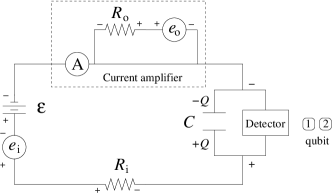
Figure 2: A schematic of our equivalent circuit for the realistic measurement of the state of a CQD charge qubit.

Our equivalent circuit for realistic measurement of the CQDs is shown in Figure 2. We emphasize that this circuit models effects of realistic measurement (additional classical noise and filtering of the signal), not an actual experimental apparatus.

The circuit is biased by a non-ideal DC voltage consisting of a noiseless voltage $\varepsilon$ and a noisy voltage source $e_{\mathrm{i}}$. This (white) noise source could be considered as the Johnson-Nyquist noise from the equivalent circuit resistance $R_{\mathrm{i}}$ at some effective temperature $T_{\rm i}$. We emphasize again that this is a model only and need not correspond to a real temperature in an actual apparatus. The small current through the detector is amplified, then measured. In this process an observer will see white noise in addition to the current through the detector. This is modeled by adding a noisy output current $e_{\mathrm{o}}/R_{\mathrm{o}}$ to the signal from the detector prior to measurement by a perfect ammeter, yielding the current ${\cal I}$. The parasitic capacitance $C$ across the detector is due to the large cross-sectional area of the leads relative to the detector junction.

Again, it is important to note that the circuit components are not necessarily representative of an actual experimental setup. For example, an amplifier does not consist of a noisy voltage and a resistor, rather the observed effect of amplification of the current through the detector can be modeled as the addition of an output noise $e_{\mathrm{o}}/R_{\mathrm{o}}$ to the current through the detector. Although our description of the circuit is rather simple, we believe that it is a reasonable starting point that models some essential effects of a realistic measurement. Future improvements to this circuit model could include considering an actual circuit from an experiment.

We analyze the equivalent circuit with the low transparency QPC as detector and produce expressions for the measured current ${\cal I}(t)$ and the time evolution of the parasitic capacitor charge $Q(t)$. The variable $Q(t)$ is used to describe the state of the circuit part of the measurement device.

For the moment, ignore tunneling through the QPC. Analysis of the measurement circuit using Kirchhoff’s electrical circuit laws yields the following Itô differential equation for the increment in $Q$ (the charge on the parasitic capacitor) due to the circuit components

$$dQ(t)=\left(-\frac{Q(t)}{R_{\mathrm{i}}C}+\frac{\varepsilon}{R_{\mathrm{i}}}+\frac{e_{\mathrm{i}}}{R_{\mathrm{i}}}\right)dt\ .$$ (11)

Similar analysis yields an expression for the measured current as a function of time:

$${\cal I}(t)=-\frac{Q(t)}{R_{\mathrm{i}}C}+\frac{\varepsilon}{R_{\mathrm{i}}}+\frac{e_{\mathrm{i}}}{R_{\mathrm{i}}}+\frac{e_{\mathrm{o}}}{R_{\mathrm{o}}}\ .$$ (12)

For the purposes of our work it is useful to express the (Johnson-Nyquist) noise sources $e_{\mathrm{i}}$ and $e_{\mathrm{o}}$ in terms of stochastic increments. In the steady state, Johnson-Nyquist voltage noise is white noise and has a flat spectrum

$$S=2k_{\mathrm{B}}TR\ ,$$ (13)

where $T$ is the temperature of the resistor $R$ and $k_{\mathrm{B}}$ is Boltzmann’s constant. The current spectrum (‘spectral density’) definitionSchoelkopf et al. (2003) used here is

$$S(\omega)=\int_{-\infty}^{\infty}\exp\left[{i\omega\tau}\right]G(\tau)d\tau\ ,$$ (14)

where $G(\tau)$ is the two-time autocorrelation function of the measured current. Obviously a current flow is not an equilibrium situation, but for reasonable bias voltages the approximation of Eq. (13) remains valid.Milburn and Sun (1998) For simplicity, we take the flat spectra of the input and output voltage noises to be $2D_{\mathrm{i}}R^{2}_{\mathrm{i}}$ and $2D_{\mathrm{o}}R^{2}_{\mathrm{o}}$, respectively. This allows us to write Eqs. (11) and (12) in terms of the input and output Wiener processes, $dW_{\mathrm{i}}(t)$ and $dW_{\mathrm{o}}(t)$, as

$$dQ(t) = \left(-\frac{Q(t)}{R_{\mathrm{i}}C}+\frac{\varepsilon}{R_{\mathrm{i}}}\right)dt+\sqrt{D_{\mathrm{i}}}dW_{\mathrm{i}}(t)\ ,$$ (15)

$${\cal I}(t) = -\frac{Q(t)}{R_{\mathrm{i}}C}+\frac{\varepsilon}{R_{\mathrm{i}}}+\sqrt{D_{\mathrm{i}}}\frac{dW_{\mathrm{i}}(t)}{dt}+\sqrt{D_{\mathrm{o}}}\frac{dW_{\mathrm{o}}(t)}{dt}\ ,$$

where $D_{\mathrm{i}}=2k_{\rm B}T_{\mathrm{i}}/R_{\mathrm{i}}$ and $D_{\mathrm{o}}=2k_{\rm B}T_{\mathrm{o}}/R_{\mathrm{o}}$. These expressions correct the expressions in Refs. Warszawski et al., 2002, Warszawski and Wiseman, 2003a and Oxtoby et al., 2003 from $4k_{\mathrm{B}}T/R$ to $2k_{\mathrm{B}}T/R$. The Wiener increment is related to Gaussian white noise $\xi(t)$ by $dW(t)=\xi(t)dt$.Gardiner (1985)

Now consider a single electron tunneling event through the QPC ($dN(t)=1$). The charge on the parasitic capacitor will change by an amount $\textrm{e}dN(t)$, where e is the charge on an electron. This gives

$$dQ(t)=\left[{-\alpha Q(t)+\beta}\right]dt+\sqrt{D_{\mathrm{i}}}dW_{\mathrm{i}}(t)+\textrm{e}dN(t),$$ (17)

where we have introduced the simplifying notations $\alpha=1/R_{\mathrm{i}}C$ and $\beta=\varepsilon/R_{\mathrm{i}}$. The solution to this differential equation gives the value of $Q(t)$ that may be substituted into Eq. (LABEL:eq:I) to give a lengthy expression for the measured current.Oxtoby et al. (2003)

IV Derivation of realistic quantum trajectories

The derivation of realistic quantum trajectories follows a number of well defined steps as presented for photodetectors in LABEL:photodetection1. We refer the reader to LABEL:photodetection1 for specific details of the derivation steps and only present the essential points and details that are unique to the solid-state situation. Note however that we use a somewhat simpler derivation, using the Zakai equation in Sec. IV.2 rather than the Kushner-Stratonovich equation of LABEL:photodetection1.

IV.1 Stochastic differential Chapman-Kolmogorov equation

Eq. (15) describes the evolution of the circuit state for situations where $Q(t)$ is known. A realistic observer will not have direct access to the precise value of $Q(t)$ due to the randomness of the microscopic events occurring within the device. We therefore require an equation for the evolution of the probability distribution for $Q$, written $P(q)$. Following the procedure outlined in LABEL:photodetection1, we obtain the stochastic differential Chapman-Kolmogorov (SDCK) equation for the evolution of $P(q)$:

$$dP^{\mu}(q) = dt\left({-\frac{\partial}{\partial q}m+\frac{D_{\mathrm{i}}}{2}\frac{\partial^{2}}{\partial q^{2}}-\sqrt{D_{\mathrm{i}}}\frac{\partial}{\partial q}dW_{\mathrm{i}}}\right)P(q)$$ (18)

$$+dN\left[{P\left({q-\textrm{e}}\right)-P(q)}\right]\ ,$$

where $m=-\alpha q+\beta$. This equation gives the increment in the probability distribution for the charge on the parasitic capacitor conditioned by the unobserved microscopic events ($\mu$) occurring within the measurement device.

IV.2 Zakai equation

The state of the circuit part of the measurement device is now represented by the probability distribution $P(q)$ that was introduced in the previous section. The state of this classical system changes upon measurement and so $P(q)$ must be updated. The best estimate of the new probability distribution representing the conditioned state of the measurement device, given a measurement result ${\cal I}$, is found using Bayesian analysisBox and Tiao (1973) to be

$$\tilde{P}(q|{\cal I})=\frac{P({\cal I}|q)P(q)}{\Lambda({\cal I})}~{},$$ (19)

where $\Lambda({\cal I})=P({\cal I}|q=\beta/\alpha)$. Here $\tilde{P}(q|{\cal I})$ is read ‘the probability of $q$ given ${\cal I}$’. The tilde denotes an unnormalized distribution and the value of $q=\beta/\alpha$ is chosen for convenience. The Zakai equation tells us how to update the probability distribution $P(q)$ when the measurement result ${\cal I}$ is obtained. The quantity $P({\cal I}|q)$ is the probability of obtaining the result ${\cal I}$ given that the state is $q$. We will use the simpler notation $P_{q}({\cal I})\equiv P({\cal I}|q)$, where the subscript denotes the result upon which the conditioning is performed. $\Lambda({\cal I})$ can be thought of as the ostensible probability distribution,Wiseman (1996) as opposed to the actual probability distribution

$$P({\cal I})=\int dqP({\cal I}|q)P(q)=\Lambda({\cal I})\int dq\tilde{P}(q|{\cal I})\ ,$$ (20)

which replaces $\Lambda({\cal I})$ in the expression for the normalized distribution $P(q|{\cal I})$.Warszawski and Wiseman (2003a)

From our expression for the measured current, Eq. (LABEL:eq:I), $P_{q}({\cal I})$ is a Gaussian distribution with a variance of $\nu=(D_{\mathrm{i}}+D_{\mathrm{o}})/dt$ and a mean of $m=-\alpha q+\beta$. Thus, Eq. (19) gives the the Zakai equation (to order $dt$):

$$\tilde{P}_{\cal I}(q)=\left[{1+{\cal I}dt\frac{m}{D_{\Sigma}}}\right]\tilde{P}(q)\ ,$$ (21)

where we have defined $D_{\Sigma}=D_{\mathrm{i}}+D_{\mathrm{o}}$ for convenience. Note that ${\cal I}$ has the ostensible distribution $\Lambda({\cal I})=\exp\left[{-{\cal I}^{2}/2\nu}\right]/\sqrt{2\pi\nu}$.

IV.3 Combining the stochastic increments

Our description of the stochastic conditional evolution of the measurement device is found by combining the increments $dP^{\mu}(q)$ and $d\tilde{P}_{{\cal I}}(q)$ given in the previous two subsections. The stochasticity of these two increments is related as the input noise $dW_{\mathrm{i}}$ plays a role in both. For this reason we must combine them into one increment using

$$\tilde{P}(q)+d\tilde{P}^{\mu}_{{\cal I}}(q)=\left[{1+{\cal I}dt\frac{m}{D_{\Sigma}}}\right]\left[{P(q)+dP^{\mu}(q)}\right]\ ,$$ (22)

rather than by simply adding them together. Remembering that we will eventually average over unobserved processes, the input noise needs to be separated into observed and unobserved parts. We express this as

$$dW_{\mathrm{i}}=a{\cal I}dt+bdW^{\prime}+cdt\ ,$$ (23)

where

$$dW^{\prime}{\cal I}dt=0\ .$$ (24)

Here $a$, $b$ and $c$ are as yet undetermined expressions and $dW^{\prime}$ is unobserved, normalized white noise that is unrelated to the known output ${\cal I}$. When averages are taken, $dW^{\prime}$ will be averaged over and ${\cal I}$ kept. The observed output [Eq. (LABEL:eq:I)] can be expressed as

$${\cal I}dt=mdt+\sqrt{D_{\mathrm{i}}}dW_{\mathrm{i}}+\sqrt{D_{\mathrm{o}}}dW_{\mathrm{o}}\ .$$ (25)

Using Eqs. (24) and (25) gives the expression for $dW^{\prime}$:

$$dW^{\prime}=\frac{\sqrt{D_{\mathrm{i}}}dW_{\mathrm{o}}-\sqrt{D_{\mathrm{o}}}dW_{\mathrm{i}}}{\sqrt{D_{\Sigma}}}\ .$$ (26)

Using this in Eq. (23) and equating the left and right hand sides allows $a$, $b$ and $c$ to be determined. Substitution of $a$, $b$ and $c$ back into Eq. (23) yields

$$dW_{\mathrm{i}} = \frac{\sqrt{D_{\mathrm{i}}}}{D_{\Sigma}}{\cal I}dt-\sqrt{\frac{D_{\mathrm{o}}}{D_{\Sigma}}}dW^{\prime}-\frac{\sqrt{D_{\mathrm{i}}}}{D_{\Sigma}}mdt\ .$$ (27)

Using this result and the SDCK equation [Eq. (18)] in Eq. (22) gives

$$P(q)+d\tilde{P}^{\mu}_{\cal I}(q) = \left\{1+dt\left({-\frac{\partial}{\partial q}m~{}+~{}\frac{D_{\mathrm{i}}}{2}\frac{\partial^{2}}{\partial q^{2}}}\right)\right.$$ (28)

$$\left.~{}+~{}\left({m-D_{\mathrm{i}}\frac{\partial}{\partial q}}\right)\frac{{\cal I}dt}{D_{\Sigma}}\right.$$

$$\left.~{}+~{}\sqrt{\frac{D_{\mathrm{i}}D_{\mathrm{o}}}{D_{\Sigma}}}\frac{\partial}{\partial q}dW^{\prime}\right\}P(q)$$

$$~{}+~{}dN\left[{P(q-\textrm{e})-P(q)}\right]\ .$$

This result represents the evolution of the circuit state conditioned on both the microscopic events occurring within the device and the observed current ${\cal I}$.

IV.4 Joint stochastic equation

The stochastic state of the joint classical-quantum system is found by forming the new conditional quantity

$$\tilde{\rho}^{\mu}_{{\cal I}}(q)=\tilde{P}^{\mu}_{{\cal I}}(q)\rho^{\mu}(t)\ .$$ (29)

The evolution of $\tilde{\rho}^{\mu}_{{\cal I}}(q)$ is described by

$$\tilde{\rho}(q)+d\tilde{\rho}_{{\cal I}}^{\mu}(q)=\big{[}\tilde{P}(q)+d\tilde{P}_{{\cal I}}^{\mu}(q)\big{]}\big{[}\rho(t)+d\rho^{\mu}(t)\big{]}\ .$$ (30)

The result of this process is the joint stochastic equationWarszawski and Wiseman (2003a)

$$d\tilde{\rho}_{{\cal I}}^{\mu}(q) = \bigg{\{}dt\left({-\frac{\partial}{\partial q}m+\frac{D_{\mathrm{i}}}{2}\frac{\partial^{2}}{\partial q^{2}}}\right)\bigg{.}$$ (31)

$$\bigg{.}+\left({m-D_{\mathrm{i}}\frac{\partial}{\partial q}}\right)\frac{{\cal I}dt}{D_{\Sigma}}+\sqrt{\frac{D_{\mathrm{i}}D_{\mathrm{o}}}{D_{\Sigma}}}\frac{\partial}{\partial q}dW^{\prime}\bigg{.}$$

$$\bigg{.}+\mathrm{E}\left[{dN}\right]+dt\bigg{(}{\cal L}-{\cal J}\left[{{{\cal T+X}\hat{n}}}\right]\bigg{)}\bigg{\}}\tilde{\rho}(q)$$

$$+~{}dN\left\{{\frac{{\cal J}\left[{{{\cal T+X}\hat{n}}}\right]\tilde{\rho}\left({q-\textrm{e}}\right)}{\mathrm{E}\left[{dN}\right]/dt}-\tilde{\rho}(q)}\right\}.$$

Averaging over unobserved processes ($dW^{\prime}$ and $dN$) is the next step in the derivation of realistic quantum trajectory equations and yields an expression for $d\tilde{\rho}_{\cal I}(q)$. This procedure removes the stochasticity associated with the unobserved processes within the detector and leaves the stochasticity associated with the measurement (${\cal I}$). The resulting equation is called a superoperator Zakai equation as we have obtained a quantum analogue of the Zakai equation in that from measurement we are conditioning the state of a super-system that contains a quantum system. It is important to realize that after averaging over unobserved processes the super-system state $\tilde{\rho}(q)+d\tilde{\rho}_{{\cal I}}(q)$ will not factorize as in Eq. (30).

IV.5 Normalization

Normalization of the superoperator Zakai equation is the final step in our derivation and yields the superoperator Kushner-Stratonovich (SKS) equation. The normalization is achieved as follows:

$$\rho(q)+d\rho_{{\cal I}}(q)=\frac{\tilde{\rho}(q)+d\tilde{\rho}_{{\cal I}}(q)}{\int\mathrm{Tr}\left[{{\tilde{\rho}_{{\cal I}}(q)+d\tilde{\rho}_{{\cal I}}(q)}}\right]dq}\ .$$ (32)

After normalization the true expression for the observed current ${\cal I}$ should be substituted into the SKS equation. The true probability distribution for ${\cal I}$ can be found using Eq. (21) in Eq. (20) to yield

$$P({\cal I})=\left({2\pi\nu}\right)^{-1/2}\exp\left[{-\left({{\cal I}+\alpha\left\langle{Q}\right\rangle-\beta}\right)^{2}/2\nu}\right]\ ,$$ (33)

where $\left\langle{Q}\right\rangle=\int qP(q)dq$. Thus, the true expression for the observed current is

$${\cal I}dt=\left({-\alpha\left\langle{Q}\right\rangle+\beta}\right)dt+\sqrt{D_{\Sigma}}d{\cal W},$$ (34)

where $d{\cal W}$ is the observed white noise (a Wiener increment). Here the average is $\left\langle{Q}\right\rangle=\int q\mathrm{Tr}\left[{{\rho_{{\cal I}}(q)}}\right]dq$, since we are considering the output ${\cal I}$ for the combined classical-quantum super-system.

Averaging over the unobserved noise $dW^{\prime}$ and tunneling process $dN$ yields the superoperator Zakai equation, which upon normalization via Eq. (32) and substitution of Eq. (34) for ${\cal I}$ produces the SKS equation:

$$d\rho_{\cal I}(q) = dt\left[{\frac{\partial}{\partial q}\left({\alpha q-\beta}\right)+\frac{D_{\mathrm{i}}}{2}\frac{\partial^{2}}{\partial q^{2}}}\right]\rho_{\cal I}(q)$$ (35)

$$-\frac{d{\cal W}}{\sqrt{D_{\Sigma}}}\left[{\alpha\left({q-\left\langle{Q}\right\rangle}\right)+D_{\mathrm{i}}\frac{\partial}{\partial q}}\right]\rho_{\cal I}(q)$$

$$+~{}dt~{}{\cal L}\rho_{\cal I}(q)$$

$$+~{}dt~{}{\cal J}\left[{{{\cal T}+{\cal X}\hat{n}}}\right]\left[{\rho_{\cal I}(q-\textrm{e})-\rho_{\cal I}(q)}\right].$$

This is the main result of our paper. The first line of Eq. (35) describes the evolution of the classical measurement device. The second line consists of two terms: the first term describes information gain about the measurement device ($q$) from its output – Eq. (34); the second term describes back-action on the classical device due to the observed noise. The third line describes the average evolution of the quantum system, including quantum back-action. The final line describes the effect of the quantum system on the measurement device.

It is worth noting that the term involving ${\cal J}$ represents average evolution due to electron tunneling events through the QPC. It changes the most likely value for the charge of the parasitic capacitor from $Q$ to $Q-\textrm{e}$ when an electron tunnels through the QPC – effectively counting the average number of electrons passing through the QPC. The approach of LABEL:Shnir98 (also used in LABEL:goan04) involves a similar technique in which the exact number of electrons that have tunneled through the detector is tracked. This was also considered in the (earlier) derivation of the rate equations in LABEL:gurvitz.

The numerical solution of Eq. (35) would produce a trajectory for the state of the combined circuit-qubit system conditioned by a particular realization of the measured current ${\cal I}(t)$. The normalized conditioned qubit state is found from

$$\rho_{{\cal I}}(t)=\int\rho_{{\cal I}}(q)dq\ .$$ (36)

Thus, the realistic quantum trajectories (for the qubit state alone) are obtained by numerically solving the SKS equation and using Eq. (36). The results of this procedure will be presented in a future paper.

V Discussion

A simple consistency check for our SKS equation [Eq. (35)] is to integrate it over all $q$ and recover the unconditional master equation. It is easy to confirm that this is indeed the case using the fact that well-behaved probability distributions (and their derivatives) vanish at $\pm\infty$.

A considerably more difficult task is to attempt recovery of the ideal conditional master equation (2) from the SKS equation (35). In theory, this should be possible in the limit of a measurement circuit with a small response time given by $R_{\mathrm{i}}C$ (large bandwidth $\alpha=\left({R_{\mathrm{i}}C}\right)^{-1}$) and low noises $D_{\mathrm{i}}$ and $D_{\mathrm{o}}$. We now explore this question in detail.

The time taken to determine which CQD is occupied by the qubit electron is equal to the time required to ascertain the rate of tunneling through the detector. This task is made considerably more difficult by the white noise and finite bandwidth of the circuit containing the detector. Without the white noise the observer would see a spike in the current every time there was a tunneling event. Depending on the relative sizes of the noise, the tunneling rates and the circuit response time, the white noise will obscure the spikes in the current so that the observer must rely on the average current to distinguish between the two qubit states. The consequence of averaging out the white noise (by integrating the current ${\cal I}$ over some time $\tau$) is that if the qubit electron is tunneling on a time scale $\Omega^{-1}$ shorter than $\tau$ then the state of the quantum system cannot be followed.

We will now present an order of magnitude estimate of the effective bandwidth of the measurement device, which is defined as the frequency at which a signal (power) to noise (power) ratio of unity is obtained. Here we take the signal as being the current that flows through the QPC when it is in the more conducting state.

To find the noise and signal power we take the Fourier transform of Eqs. (LABEL:eq:I) and (17) in order to obtain the spectrum of the current ${\cal I}$.Oxtoby et al. (2003) The signal power is

$$r^{\prime}\textrm{e}^{2}\frac{\alpha^{2}}{\alpha^{2}+\omega^{2}}$$ (37)

and the noise power is

$$D_{\mathrm{i}}\frac{\omega^{2}}{\alpha^{2}+\omega^{2}}+D_{\mathrm{o}}\ .$$ (38)

Upon equating the signal and noise powers, and at this frequency setting $\omega=\alpha_{\mathrm{eff}}$, we have an effective bandwidth of

$$\alpha_{\mathrm{eff}}=\frac{\alpha}{\sqrt{\mathbf{N}}}\sqrt{1-\frac{D_{\mathrm{o}}}{r^{\prime}\textrm{e}^{2}}}\approx\frac{\alpha}{\sqrt{\mathbf{N}}}\ ,$$ (39)

where the dimensionless noise parameter N is defined according to

$$\mathbf{N}=\frac{\left({D_{\mathrm{i}}+D_{\mathrm{o}}}\right)}{r^{\prime}\textrm{e}^{2}}\ .$$ (40)

The approximation of Eq. (39) holds in the limit where the noise power $D_{\mathrm{o}}$ is small compared to the signal power $r^{\prime}\textrm{e}^{2}$ (which is the regime that will lead to good measurements of the qubit state). For an observer to be able to follow the evolution of the qubit reasonably well we must have $\alpha_{\mathrm{eff}}>\Omega$.Warszawski and Wiseman (2003a, b)

VI Conclusion

VI.1 Summary

We have presented a new model for continuous measurement of a coupled quantum dot (CQD) charge qubit by a low transparency quantum point contact (QPC). We considered the evolution of this solid-state qubit conditioned on the output available to a realistic observer, which has been filtered and degraded (i.e. made more noisy) by an external circuit. This description is closer to the true conditioned evolution of the system, not a hypothetical evolution conditioned on the microscopic events occurring within the detector, to which a real observer has no direct access. Knowledge of the state of a quantum system conditioned on actual measurement results is essential for understanding and designing feedback control.Wiseman and Milburn (1993a); Wiseman (1995); Armen et al. (2002); Doherty and Jacobs (1999); Doherty et al. (2000); Wiseman et al. (2002); Smith et al. (2002); Korotkov (2001a); Ruskov and Korotkov (2002) It is also expected to be important in quantum computing, both for state preparation and quantum error correction.Ahn et al. (2003); Sarovar et al. (2004); Ahn et al. (2004)

Our model for the conditional dynamics of the qubit due to measurement by a low transparency quantum point contact (QPC) was based on the quantum trajectory models of Refs. Wiseman et al., 2001 and Goan et al., 2001. We have presented a stochastic master equation that describes the time evolution of the measured qubit conditioned on a hypothetical detector output. Korotkov has derived equivalent conditional dynamics equations for the QPC (with notational differences) using a Bayesian formalism.Korotkov (1999, 2001a, 2001b, 2003a, 2003b) We generalized a realistic quantum trajectory theoryWarszawski et al. (2002); Warszawski and Wiseman (2003a) (recently developed for photodetectors) to treat solid-state detectors. The solutions of the resulting stochastic equations are the “realistic quantum trajectories” of the measured qubit state. These will be presented elsewhere.

VI.2 Comparison to previous work

The conditional dynamics of continuously monitored CQD systems has been studied in Refs. Korotkov, 1999, 2001a, 2001b; Wiseman et al., 2001; Goan et al., 2001; Goan and Milburn, 2001; Korotkov, 2003a, b; Gurvitz et al., 2003. However, the model of realistic measurement that we have presented in this paper is new. Korotkov has recently presented a phenomenological theoryKorotkov (2003a) involving “non-ideal” detectors that is in the same spirit as ours (see Appendix A for a derivation of Korotkov’s result using our stochastic master equation approach). However, he still assumed an infinite bandwidth detector and also assumed that the ideal detector could be described by diffusion rather than jumps. We believe that our approach offers a more satisfying description of this measurement process because the non-Markovian effects of a realistic measurement circuit are included and the tunneling process through the QPC is described as a point process (jumps) as one would expect.

Finite detector temperature effects in the case of bare measurement were not considered in our model. The effects of a non-zero detector temperature $T_{\mathrm{d}}$ have been considered previouslyGoan et al. (2001); Korotkov (2001a); Ruskov and Korotkov (2003) and result in an approximately linear ($\coth\left[{\textrm{e}V_{\mathrm{d}}/2k_{\mathrm{B}}T_{\mathrm{d}}}\right]$) increase in the ensemble decoherence rate and shot noise level with $T_{\mathrm{d}}$ for $\textrm{e}V_{\mathrm{d}}<2k_{\mathrm{B}}T_{\mathrm{d}}$, where $V_{\mathrm{d}}$ is the detector bias voltage. With a detector temperature of the order of mK,Grabert and Devoret (1992) finite temperature effects could be expected to become important at bias voltages of $V_{\mathrm{d}}<0.3\mu V$. These voltages are several orders of magnitude below a sample bias voltage for maximum response of a single electron transistor (SET) detecting the charge state of a quantum dot,Berman et al. (1997, 1999) which suggests that our omission of finite detector temperature effects in the bare detector scenario is reasonable.

VI.3 Future Work

There are many possibilities for future work in the theory of realistic quantum trajectories. Other detectors will be considered – for example, the single electron transistorFulton and Dolan (1987); Averin and Likharev (1986) (SET). As the field of mesoscopic electronics is progressing at such a tremendous rate it is likely that the choice of detector will quickly become outdated. In fact, the SET has already been surpassed by the radio-frequency (RF) SETSchoelkopf et al. (1998); Fujisawa and Hirayama (2000); Devoret and Schoelkopf (2000) as the measuring device of choice for the read out of the charge state of a mesoscopic qubit. This is one reason why we view the work in this paper as preliminary. The extension of realistic quantum trajectories to the RF-SET is a future aim.

Further work is also appropriate for the circuit model, which at present is considerably simplified, but is a good starting point which models some essential effects of a realistic measurement.

These and other possibilities for work on the theory of realistic quantum trajectories will be pursued in the future.

Appendix A Derivation of Korotkov’s result using our approach

In this appendix we derive an equivalent result to Korotkov’s phenomenological result for non-ideal detectorsKorotkov (2003a) using a diffusive stochastic master equation approach and our method involving observed and unobserved noises.

We begin by defining a diffusive linear stochastic master equationWiseman (1996) for the state matrix of a measured two level system. The Itô stochastic master equation involving three classical, normalized white noise processes $dW_{0}$ (ideal detector output noise), $dW_{1}$ (extra output and back-action noise) and $dW_{3}$ (unobserved back-action noise) is

$$d\tilde{\rho} = dt{\cal L}\tilde{\rho}~{}+~{}dW_{0}\sqrt{\kappa_{0}}~{}\left({\hat{\sigma}_{z}\tilde{\rho}+\tilde{\rho}\hat{\sigma}_{z}}\right)$$

$$+~{}dW_{1}\sqrt{\kappa_{1}}~{}{\cal H}\left[{{-i\hat{\sigma}_{z}}}\right]\tilde{\rho}+~{}dW_{3}\sqrt{\kappa_{3}}~{}{\cal H}\left[{{-i\hat{\sigma}_{z}}}\right]\tilde{\rho}\ ,$$

where ${\cal L}={\cal H}\left[{{-i\hat{H}}}\right]+\left({\kappa_{0}+\kappa_{1}+\kappa_{3}}\right){\cal D}\left[{{\hat{\sigma}_{z}}}\right]$ and $\hat{H}=\Omega\hat{\sigma}_{x}+\mbox{$\frac{1}{2}$}\varepsilon\hat{\sigma}_{z}$. Eq. (9) defines the superoperator ${\cal H}$.

The three white noise processes $dW_{0}$, $dW_{1}$ and $dW_{3}$ correspond to Korotkov’s three unnormalized noise processes $\xi_{0}(t)$, $\xi_{1}(t)$ and $\xi_{3}(t)$. The white noise $dW_{0}/dt$ represents the output of an ideal detector. Korotkov’s added output noise is known as dark noise, which we model by setting the output of the realistic detector to be the current

$${\cal I}(t)dt=\left({\sqrt{\phi_{0}}dW_{0}+\sqrt{\phi_{1}}dW_{1}}\right)/\sqrt{\phi_{\Sigma}}\ ,$$ (42)

where $\phi_{0}$ is the shot noise power, $\phi_{1}$ is the dark noise power and $\phi_{\Sigma}\equiv\phi_{0}+\phi_{1}$ ensures that ${\cal I}(t)$ has a normalized Gaussian white noise distribution.

We now desire the quantum trajectory for the system state $\rho_{\cal I}$ conditioned on the realistic detector output in Eq. (42) rather than on $dW_{0}/dt$. We rewrite $dW_{0}$ as

$$dW_{0}=\left({\sqrt{\phi_{0}}{\cal I}(t)dt+\sqrt{\phi_{1}}dW^{\prime}}\right)/\sqrt{\phi_{\Sigma}}\ ,$$ (43)

where $dW^{\prime}=\left({\sqrt{\phi_{1}}dW_{0}-\sqrt{\phi_{0}}dW_{1}}\right)/\sqrt{\phi_{\Sigma}}$ is an unobserved normalized noise process that is independent of the observed output ${\cal I}(t)$. The extra output noise $dW_{1}$ can be expressed in terms of observed and unobserved quantities as

$$dW_{1}=\left({\sqrt{\phi_{1}}{\cal I}(t)dt-\sqrt{\phi_{0}}dW^{\prime}}\right)/\sqrt{\phi_{\Sigma}}\ .$$ (44)

Substituting these into Eq. (LABEL:eq:linearSME) yields

$$d\tilde{\rho} = dt{\cal L}\tilde{\rho}~{}+~{}\frac{{\sqrt{\phi_{0}}{\cal I}(t)dt+\sqrt{\phi_{1}}dW^{\prime}}}{\sqrt{\phi_{\Sigma}}}\sqrt{\kappa_{0}}~{}\left({\hat{\sigma}_{z}\tilde{\rho}+\tilde{\rho}\hat{\sigma}_{z}}\right)$$ (45)

$$+~{}\frac{{\sqrt{\phi_{1}}{\cal I}(t)dt-\sqrt{\phi_{0}}dW^{\prime}}}{\sqrt{\phi_{\Sigma}}}\sqrt{\kappa_{1}}~{}{\cal H}\left[{{-i\hat{\sigma}_{z}}}\right]\tilde{\rho}$$

$$+~{}dW_{3}\sqrt{\kappa_{3}}~{}{\cal H}\left[{{-i\hat{\sigma}_{z}}}\right]\tilde{\rho}\ .$$

Averaging over the unobserved noise processes $dW^{\prime}$ and $dW_{3}$ removes the terms involving $dW^{\prime}$ and $dW_{3}$ from Eq. (45). Normalization of this result is performed in a similar manner as in Sec. IV.5 with the final result being the following non-linear SME:

$$d\rho = dt{\cal L}\rho+\sqrt{\frac{\kappa_{0}\phi_{0}}{\phi_{\Sigma}}}dt\left({{\cal I}(t)-2\left\langle{\hat{\sigma}_{z}}\right\rangle\sqrt{\frac{\kappa_{0}\phi_{0}}{\phi_{\Sigma}}}}\right)~{}{\cal H}\left[{{\hat{\sigma}_{z}}}\right]\rho$$

$$+dt\sqrt{\frac{\kappa_{1}\phi_{1}}{\phi_{\Sigma}}}\left({{\cal I}(t)-2\left\langle{\hat{\sigma}_{z}}\right\rangle\sqrt{\frac{\kappa_{0}\phi_{0}}{\phi_{\Sigma}}}}\right)~{}{\cal H}\left[{{-i\hat{\sigma}_{z}}}\right]\rho\ .$$

Now we substitute in for the actual measured current, ${\cal I}(t)dt=2\left\langle{\hat{\sigma}_{z}}\right\rangle\sqrt{\kappa_{0}\phi_{0}/\phi_{\Sigma}}dt+d{\cal W}$, to obtain

$$d\rho = dt{\cal L}\rho+\sqrt{\frac{\kappa_{0}\phi_{0}}{\phi_{\Sigma}}}~{}d{\cal W}~{}{\cal H}\left[{{\hat{\sigma}_{z}}}\right]\rho$$ (47)

$$+\sqrt{\frac{\kappa_{1}\phi_{1}}{\phi_{\Sigma}}}~{}d{\cal W}~{}{\cal H}\left[{{-i\hat{\sigma}_{z}}}\right]\rho\ ,$$

which is equivalent to the non-ideal result of Korotkov in LABEL:korotkov03 with some notational differences.

References

- Kane (1998) B. E. Kane, Nature (London) 393, 133 (1998).
- Loss and DiVincenzo (1998) D. Loss and D. P. DiVincenzo, Phys. Rev. A 57, 120 (1998).
- Privman et al. (1998) V. Privman, I. D. Vagner, and G. Kventsel, Phys. Lett. A 239, 141 (1998).
- Imamoḡlu et al. (1999) A. Imamoḡlu, D. D. Awschalom, G. Burkard, D. P. DiVincenzo, D. Loss, M. Sherwin, and A. Small, Phys. Rev. Lett. 83, 4204 (1999).
- Vrijen et al. (2000) R. Vrijen, E. Yablonovitch, K. Wang, H. W. Jiang, A. Balandin, V. Roychowdhury, T. Mor, and D. DiVincenzo, Phys. Rev. A 62, 012306 (2000).
- DiVincenzo (1995) D. P. DiVincenzo, Science 270, 255 (1995).
- Burkard and Loss (2002) G. Burkard and D. Loss, Europhysics News 33 (2002).
- Vandersypen et al. (2003) L. M. K. Vandersypen, R. Hanson, L. H. Willems van Beveren, J. M. Elzerman, J. N. Griedanus, S. De Franceschi, and L. P. Kouwenhoven, in Quantum Computing and Quantum Bits in Mesoscopic Systems, edited by A. J. Leggett, B. Ruggiero, and P. Silvestrini (Kluwer Academic/Plenum Publishers, New York, 2003).
- Gurvitz (1997) S. A. Gurvitz, Phys. Rev. B 56, 15215 (1997).
- Shnirman and Schön (1998) A. Shnirman and G. Schön, Phys. Rev. B 57, 15400 (1998).
- Korotkov (1999) A. N. Korotkov, Phys. Rev. B 60, 5737 (1999); 63 085312 (2001).
- Korotkov (2001a) A. N. Korotkov, Phys. Rev. B 63, 115403 (2001a).
- Wiseman et al. (2001) H. M. Wiseman, Dian Wahyu Utami, H. B. Sun, G. J. Milburn, B. E. Kane, A. Dzurak, and R. G. Clark, Phys. Rev. B 63, 235308 (2001).
- Goan et al. (2001) H.-S. Goan, G. J. Milburn, H. M. Wiseman, and H. B. Sun, Phys. Rev. B 63, 125326 (2001).
- Korotkov (2001b) A. N. Korotkov, Phys. Rev. B 64, 193407 (2001b).
- Goan and Milburn (2001) H.-S. Goan and G. J. Milburn, Phys. Rev. B 64, 235307 (2001).
- Korotkov (2003a) A. N. Korotkov, Phys. Rev. B 67, 235408 (2003a).
- Korotkov (2003b) A. N. Korotkov, in Quantum Noise in Mesoscopic Physics, edited by Y. V. Nazarov (Kluwer Academic, Netherlands, 2003b), pp. 205–228.
- Gurvitz et al. (2003) S. A. Gurvitz, L. Fedichkin, D. Mozyrsky, and G. P. Berman, Phys. Rev. Lett. 91, 066801 (2003).
- Wiseman and Milburn (1993a) H. M. Wiseman and G. J. Milburn, Phys. Rev. Lett. 70, 548 (1993a).
- Wiseman (1995) H. M. Wiseman, Phys. Rev. Lett. 75, 4587 (1995).
- Doherty and Jacobs (1999) A. C. Doherty and K. Jacobs, Phys. Rev. A 60, 2700 (1999).
- Doherty et al. (2000) A. C. Doherty, S. Habib, K. Jacobs, H. Mabuchi, and S. M. Tan, Phys. Rev. A 62, 012105 (2000).
- Armen et al. (2002) M. A. Armen, J. K. Au, J. K. Stockton, A. C. Doherty, and H. Mabuchi, Phys. Rev. Lett. 89, 133602 (2002).
- Wiseman et al. (2002) H. M. Wiseman, S. Mancini, and J. Wang, Phys. Rev. A 66, 013807 (2002).
- Smith et al. (2002) W. P. Smith, J. E. Reiner, L. A. Orozco, S. Kuhr, and H. M. Wiseman, Phys. Rev. Lett. 89, 133601 (2002).
- Ruskov and Korotkov (2002) R. Ruskov and A. N. Korotkov, Phys. Rev. B 66, 041401(R) (2002).
- Ahn et al. (2003) C. Ahn, H. M. Wiseman, and G. J. Milburn, Phys. Rev. A 67, 052310 (2003).
- Sarovar et al. (2004) M. Sarovar, C. Ahn, K. Jacobs, and G. J. Milburn, Phys. Rev. A 69, 052324 (2004).
- Ahn et al. (2004) C. Ahn, H. M. Wiseman, and K. Jacobs, Phys. Rev. A 70, 024302 (2004).
- Carmichael (1993) H. J. Carmichael, An Open Systems Approach to Quantum Optics (Springer, Berlin, 1993).
- Wiseman and Milburn (1993b) H. M. Wiseman and G. J. Milburn, Phys. Rev. A 47, 1652 (1993b).
- Wiseman (1996) H. M. Wiseman, Quantum Semiclass. Opt. 8, 205 (1996).
- Warszawski et al. (2002) P. Warszawski, H. M. Wiseman, and H. Mabuchi, Phys. Rev. A 65, 023802 (2002).
- Warszawski and Wiseman (2003a) P. Warszawski and H. M. Wiseman, J. Opt. B: Quantum Semiclass. Opt. 5, 1 (2003a).
- Field et al. (1993) M. Field, C. G. Smith, M. Pepper, D. A. Ritchie, J. E. F. Frost, G. A. C. Jones, and D. G. Hasko, Phys. Rev. Lett. 70, 1311 (1993).
- Gardiner (1985) C. W. Gardiner, Handbook of Stochastic Methods for the Physical Sciences (Springer, Berlin, 1985).
- Braginsky and Khalili (1992) V. B. Braginsky and F. Y. Khalili, Quantum Measurement (Cambridge University Press, 1992).
- Goan (2004) H.-S. Goan, Phys. Rev. B 70, 075305 (2004).
- Schoelkopf et al. (2003) R. J. Schoelkopf, A. A. Clerk, S. M. Girvin, K. W. Lehnert, and M. H. Devoret, in Noise and Information in Nanoelectronics, Sensors and Standards, edited by L. B. Kish, F. Green, G. Iannaccone, and J. R. Vig (SPIE, 2003), vol. 5115, pp. 356–376.
- Milburn and Sun (1998) G. J. Milburn and H. B. Sun, Contemporary Physics 39, 1, 67 (1998).
- Oxtoby et al. (2003) N. P. Oxtoby, H.-B. Sun, and H. M. Wiseman, J. Phys.: Condens. Matter 15, 8055 (2003).
- Box and Tiao (1973) G. E. P. Box and G. C. Tiao, Bayesian Inference in Statistical Analysis (Addison-Wesley, Sydney, 1973).
- Warszawski and Wiseman (2003b) P. Warszawski and H. M. Wiseman, J. Opt. B: Quantum Semiclass. Opt. 5, 15 (2003b).
- Ruskov and Korotkov (2003) R. Ruskov and A. N. Korotkov, Phys. Rev. B 67, 075303 (2003).
- Grabert and Devoret (1992) H. Grabert and M. H. Devoret, eds., Single Charge Tunneling: Coulomb Blockade Phenomena in Nanostructures (Plenum Press, New York, 1992).
- Berman et al. (1997) D. Berman, N. B. Zhitenev, R. C. Ashoori, H. I. Smith, and M. R. Melloch, J. Vac. Sci. Technol. B 15, 2844 (1997).
- Berman et al. (1999) D. Berman, N. B. Zhitenev, R. C. Ashoori, and M. Shayegan, Phys. Rev. Lett. 82, 161 (1999).
- Fulton and Dolan (1987) T. A. Fulton and G. J. Dolan, Phys. Rev. Lett. 59, 109 (1987).
- Averin and Likharev (1986) D. V. Averin and K. K. Likharev, J. Low Temp. Phys. 62, 345 (1986).
- Schoelkopf et al. (1998) R. J. Schoelkopf, P. Wahlgren, A. A. Kozhevnikov, P. Delsing, and D. E. Prober, Science 280, 1238 (1998).
- Fujisawa and Hirayama (2000) T. Fujisawa and Y. Hirayama, Appl. Phys. Lett. 77, 543 (2000).
- Devoret and Schoelkopf (2000) M. H. Devoret and R. J. Schoelkopf, Nature 406, 1039 (2000).