Dynamical localization for Bloch electrons in Magnetic and Electric Fields

Abstract

We study the time evolution of wave packets of noninteracting electrons in a two-dimensional periodic system in the presence of magnetic and electric fields. The model includes consistently the coupling between Landau levels as well as the periodic and external field contributions. It is shown that the electric field produces localization along its longitudinal direction, this effect is a physical consequence of the quantization of the energy levels with respect to the longitudinal quasi-momentum. For incommensurate orientations of $\mathbf{E}$ relative to the lattice the wave packet becomes localized in both direction.

Localization of waves in quasiperiodic system has been the subject of great interest in condensed matter and related areas in physics. An electron subject to a sum of potentials which are periodic but incommensurate with one another represents a case that is intermediate between a random and a perfectly ordered system. In an incommensurate situation there can be both localized and extended states, with the intermediate possibility of a metal-insulator transition as the energy and-or the strength of the potential are varied. Aubry and Andre [1] presented a one-dimensional model that exhibits this behavior; the dynamics of their model is governed by the Harper [2]. The same model also arises in the the study of an electron moving in a two-dimensional lattice subject to a magnetic field, both in the limiting cases of either a very large [2] or a very small [3] potential strength compared to the magnetic field intensity. The problem of electrons moving under the simultaneous influence of a periodic potential and a magnetic field has been discussed by many authors [2, 3, 4, 5]; the spectrum displays an amazing complexity including various kinds of scaling and a Cantor set structure [6]. The addition of an electric field leads to interesting new phenomena that makes its analysis worthwhile. For example, as the strength of the electric field increases the longitudinal quasi-momentum is quantized leading to the appearance of a ”magnetic Stark ladder” in which the bands are replaced by a series of quasi discreet levels [7, 8]. The object of the present work is to study the time evolution of electron wave packets in a periodic two dimensional system subject to external electric and magnetic fields. Previous studies of this problem were usually restricted to a single band limit derived from a tight binding and/or the Peirles approximations [9, 10]. Here we presents a model which consistently includes the coupling between Landau levels as well as the periodic and external field contributions. This treatment becomes essential if one would like to analyze physical realistic situations. The study of these phenomena has become experimentally accessible with the recent developments in the fabrication of antidot arrays in lateral superlattices by ion beam and atomic force lithography [11, 12]. For example, the observation of the Hofstadter Butterfly spectrum through the measurement of the magnetoresistance and Hall conductance in artificial arrays of anti quantum dots has just been achieved [13].

We consider the motion of an electron in a two-dimensional periodic potential $V\left(x,y\right)$ subject to a uniform magnetic field $\mathbf{B}$ perpendicular to the plane and to a constant electric field $\mathbf{E}$, lying on the plane according to $\mathbf{E}=E\,(cos\theta,sin\theta)$, with $\theta$ the angle between $\mathbf{E}$ and the lattice $x-$axis. The dynamic is governed by the Schrödinger equation

$$i\hbar\frac{\partial}{\partial t}\psi=\left[\frac{1}{2m}\left(\mathbf{p}+e\mathbf{A}\right)^{2}-e\phi\left(x,y\right)+V\left(x,y\right)\right]\psi,$$ (1)

the vector and scalar potentials are selected to yield: $\nabla\times\mathbf{A}=B\hat{k}$, and $\mathbf{E}=-\nabla\phi-\partial\mathbf{A}/\partial t$. For simplicity we shall consider a periodic square lattice: $V\left(x,y\right)=U_{0}\left[\cos\left(2\pi x/a\right)+\lambda\cos\left(2\pi y/a\right)\right].$ Two characteristic parameters of the system, the cyclotron frequency $\omega_{c}=eB/m$ and the magnetic length $l_{B}=\sqrt{\hbar/(eB)}$ set the reference scales for energy and lengths respectively. Following the formalism developed in references [7, 8], we introduce a canonical transformation to new variables $Q,P$, acoording to

$$Q_{0} =t\,, P_{0}=i\hbar\partial_{t}+e\tilde{\phi}+\frac{m}{2}\left(|\mathbf{E}|/B\right)^{2},$$

$$eQ_{1} =p_{y}+eA_{y}+mE_{x}/B\,, P_{1}=p_{x}+A_{x}-mE_{y}/B,$$

$$eQ_{2} =p_{x}+e\tilde{A}_{x}-E_{x}t\,, P_{2}=p_{y}+e\tilde{A}_{y}-E_{y}t,$$ (2)

where $\tilde{\phi}=\phi+\mathbf{r}\cdot\mathbf{E}$, $\tilde{A}_{x}=A_{x}+By+E_{x}t$ and $\tilde{A}_{y}=A_{y}+Bx+E_{y}t$. It is easily verified that the transformation is indeed canonical, the new variables obey the commutation rules: $\left[Q_{0},P_{0}\right]=-i\hbar$, and $\left[Q_{1},P_{1}\right]=\left[Q_{2},P_{2}\right]=i\hbar B$; all other commutators being zero. The inverse transformation gives $x=l_{B}^{2}\left(eQ_{1}-P_{2}\right)/\hbar$ and $y=l_{B}^{2}\left(eQ_{2}-P_{1}\right)/\hbar$. The operators $(P_{0},Q_{2},P_{2})$ can be identified with the generators of the electric-magnetric translation simetries [14, 7]. Final results are independent of the selected gauge. From the operators in Eq. (2) we construct two pairs of harmonic oscillator-like ladder operators: $(a_{1},a_{1}^{{\dagger}})$, and $(a_{2},a_{2}^{{\dagger}})$ with :

$$a_{1}=\sqrt{\frac{1}{2\hbar B}}\left(P_{1}-iQ_{1}\right),\qquad a_{2}=\sqrt{\frac{1}{2\hbar B}}\left(P_{2}-iQ_{2}\right),$$ (3)

obeying: $[a_{1},a_{1}^{{\dagger}}]=[a_{2},a_{2}^{{\dagger}}]=1$, and $[a_{1},a_{2}]=[a_{1},a_{2}^{{\dagger}}]=0$. Using these variables, the Schrödinger equation can be recast as $P_{0}\left|\psi\right\rangle=H\left|\psi\right\rangle$ with the Hamiltonian given by

$$H=\hbar\omega_{c}\left(\frac{1}{2}+a_{1}^{{\dagger}}a_{1}\right)+V-el_{B}\left(\tilde{E}a_{2}+\tilde{E}^{*}a_{2}^{{\dagger}}\right),$$ (4)

here $\tilde{E}=(E_{x}+iE_{y})/\sqrt{2}$, and $V(x,y)\equiv V(Q_{1}-P_{2},Q_{2}-P_{1})$ has to be expressed in terms of the ladder operators using Eq. (3). The properties of the system depends on five dimensionless parameters: (i) $\lambda$ modulates the relative potential amplitudes in $x$ and $y$ directions, $\lambda>1$ ($\lambda<1$) corresponds to a weaker modulation along the $x$ ($y$) direction. (ii) $\sigma^{-1}=\phi/\phi_{0}=a^{2}B/(h/e)$ is the number of flux quanta in a unit cell of area $a^{2}$. (iii) $\theta$ is the relative angle between the electric field direction and the lattice $x-$axis. The two other parameters $K$ and $\rho$ are the potential strength in units of $\hbar\,\omega_{c}$, and the electric field in units of $U_{0}/(ea)$, hence: (iv) $K=U_{0}/\hbar\,\omega_{c}$, and (v) $\rho=ea|\vec{E}|/U_{0}$, respectively. As an appropriate set of basis functions we choose the eigenstates of the number operators $a_{1}^{{\dagger}}a_{1}$ and $a_{2}^{{\dagger}}a_{2}$

$$a_{1}^{{\dagger}}a_{1}\left|\mu,\nu\right\rangle =\mu\left|\mu,\nu\right\rangle, a_{2}^{{\dagger}}a_{2}\left|\mu,\nu\right\rangle =\nu\left|\mu,\nu\right\rangle,$$ (5)

where $\mu$ labels the Landau levels and $\left|\mu,\nu\right\rangle=\left|\mu\right\rangle\otimes\left|\nu\right\rangle$. These states are also eigenvectors of the angular momentum operator $\mathcal{J}=(P_{1}^{2}+Q_{1}^{2}-P_{2}^{2}-Q_{2}^{2})/2$: $\mathcal{J}\left|\mu,\nu\right\rangle=\hbar\left(\mu-\nu\right)\left|\mu,\nu\right\rangle.$ In the coordinate representation the wave function for this state takes the form

$$\psi_{\mu,\nu}\left(x,y\right)=\frac{e^{-\left(x^{2}+y^{2}\right)/4l_{B}^{2}}}{\sqrt{2\pi}}i^{\nu}\sqrt{\frac{2^{\mu}\mu!}{2^{\nu}\nu!}}\left(\frac{x+iy}{l_{B}}\right)^{\nu-\mu}L_{\mu}^{\nu-\mu}\left[\frac{\left(x^{2}+y^{2}\right)}{2l_{B}^{2}}\right],$$ (6)

where $L_{\mu}^{\nu-\mu}$ are the generalized Laguerre polynomials, the previous formula is valid for $\mu\leq\nu$, if $\mu\geq\nu$ the indices $\mu$ and $\nu$ must be exchanged on the right hand side. These wave functions are centered in the origin and its mean square radius is given by $\left\langle\mu,\nu\left|r^{2}\right|\mu,\nu\right\rangle=8\,l_{B}^{2}\,\left(\mu+\nu+1\right).$ The initial form of the wave packet has been selected as the lowest Landau level with zero angular momentum: $\psi_{0,0}\left(x,y\right)$. The evolution of the system is obtained applying the operator $O\left(t\right)=\exp\left(-itH\right)$ to the initial state $i.e.$ $\Psi\left(t,x,y\right)=\left\langle x,y\left|O\left(t\right)\right|0,0\right\rangle.$ The Hamiltonian in (4) is represented by a matrix $\mathbb{H}$ with elements evaluated in the base given in Eq. (5), the matrix elements can be worked out as

$$\left\langle\mu^{\prime},\nu^{\prime}\left|H\right|\mu,\nu\right\rangle=\\ \delta_{\mu^{\prime},\mu}\bigg{[}\hbar\omega_{c}\left(\frac{1}{2}+\mu\right)\delta_{\nu^{\prime},\nu}-el_{B}\left(\tilde{E}\sqrt{\nu^{\prime}}\delta_{\nu^{\prime},\nu+1}+\tilde{E}^{*}\sqrt{\nu}\delta_{\nu^{\prime}+1,\nu}\right)\bigg{]}+\\ U_{0}\bigg{[}D_{\mu^{\prime},\mu}\left(\sqrt{\pi\sigma}\right)D_{\nu^{\prime},\nu}\left(-i\sqrt{\pi\sigma}\right)+\lambda D_{\mu^{\prime},\mu}\left(-i\sqrt{\pi\sigma}\right)D_{\nu^{\prime},\nu}\left(\sqrt{\pi\sigma}\right)+\mathrm{c.c.}\bigg{]},\\$$ (7)

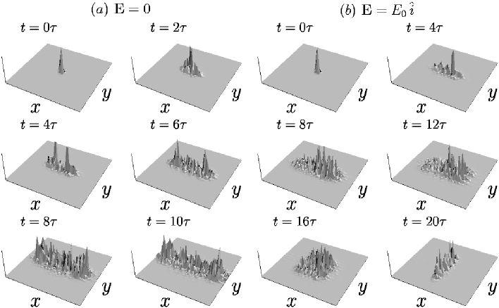
Figure 1: Time evolution of an initially localized wave packet in a $2D$ periodic asymmetric potential ($\lambda=2$; lower modulation amplitude in the $x$ direction) for: (a) $\mathbf{E}=0$, and (b) an electric field pointing in the $x$ direction, with an intensity $\rho=ea|\vec{E}|/U_{0}=0.1$. Time is measured in units of $\tau=2\pi/\omega_{c}$. Here and throughout the paper the value of the other parameters are $\sigma=1/2$, $K=5.5$.

where $D_{\mu^{\prime},\mu}\left(z\right)=\left\langle\mu^{\prime}\left|e^{za_{1}-z^{*}a^{{\dagger}}_{1}}\right|\mu\right\rangle=\psi_{\mu^{\prime},\mu}\left(\sqrt{2}\mathrm{Re}z,\sqrt{2}\mathrm{Im}z\right)$ are the matrix elements of the coherent state operator $e^{(za_{1}-z^{*}a^{{\dagger}}_{1})}$, they can be expressed using the same functions that determine the wave function profiles (Eq. 6). The Hamiltonian in (7) is diagonalized numerically by the unitary matrices $\mathbb{U}$ that are constructed from the column eigenvectors of $\mathbb{H}$. In this base the evolution operator takes the form $\mathbb{O}\left(t\right)=\mathbb{U}^{{\dagger}}\exp{\left(-it\mathbb{E}\right)}\mathbb{U},$ where $\mathbb{E}$ is the diagonal matrix containing the energy eigenvalues. The time evolution of the system is given by

$$\Psi\left(t,x,y\right)=\sum_{\mu,\nu=0}^{\infty}\mathbb{C}^{\mu}_{\nu}\left(t\right)\psi_{\mu,\nu}\left(x,y\right),$$ (8)

where $\mathbb{C}\left(t\right)=\mathbb{O}\left(t\right)\mathbb{C}\left(0\right)$, with the initial state $\mathbb{C}^{\mu}_{\nu}\left(0\right)=\delta_{\mu,0}\delta_{\nu,0}$. A global characterization of the dynamic evolution of a wave packet is provided by displaying $3\,D$ graphics of the probability density $\rho\left(t,x,y\right)=\left|\Psi\left(t,x,y\right)\right|^{2},$ as a function of the space-time variables. The localization properties of the system are characterized by the evolution of the mean square displacement $\sigma^{2}_{r}(t)$. Both the electric field and the $\lambda$ parameter can induce anisotropy transport properties, so its is sometimes convenient to separately refer to the $x$ and $y$ variance: $\sigma_{x}^{2}\left(t\right)=\left\langle x^{2}\right\rangle_{t}-\left\langle x\right\rangle^{2}_{t},$ and $\sigma_{y}^{2}\left(t\right)=\left\langle y^{2}\right\rangle_{t}-\left\langle y\right\rangle^{2}_{t},$ with $\sigma^{2}_{r}=\sigma^{2}_{x}+\sigma^{2}_{y}$. As an additional criteria we consider the Shannon information entropy[15], defined by

$$S\left(t\right)=-\int\rho(t,\vec{r})\,\,\ln\rho(t,\vec{r})\,\,d^{2}r.$$ (9)

This quantity characterize the spreading of the probability density distribution, it provides a measure of the spatial delocalization of the wave packet. The lower this quantity is, the more localized the electron is.

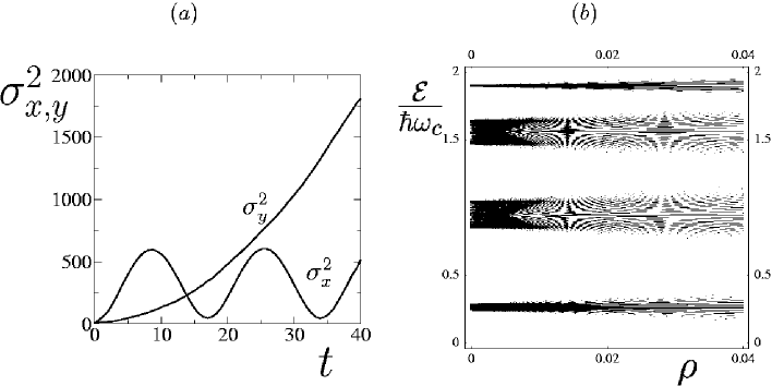
Figure 2: (a) Time evolution of the $\sigma_{x}^{2}$ and $\sigma_{y}^{2}$ variances for the wave packet represented in Fig. 1b, the wave packet is dynamically localized in the longitudinal direction and spreads ballistically in the direction of stronger modulation $\sigma_{y}^{2}\sim t^{2}$. (b) Energy subspectra as a function of the parameter $\rho$ ($\rho=ea|\vec{E}|/U_{0}$). The transverse quasimomentum is fixed to $k_{y}=0$ and the longitudinal quasimomentum takes all possible values in the first Brillouin zone, $k_{x}\in(-\pi/2a,+\pi/2a)$. The first two Landau levels are shown, $\sigma=1/2$, so every Landau level splits in two bands. A transition from extended to localized states is observed as the electric field intensity is increased.

In what follows we analyze the propagation of wave packets and its properties for some specific examples. Using the Peirls tight-binding model Nazareno and Brito [9] studied the electron wave propagation, they found that for $\sigma$ rational the electron propagates ballistically, whereas for irrational $\sigma$ the wave remains localized. Using our model that incorporates inter-Landau couplings, we have verified that these results remain valid; details are not presented due to space limitations. In what follows we shall restrict to the case of $\sigma=1/2$ and fix the parameter $K$ to $K=5.5$. The Hamiltonian in (7) is diagonalized numerically considering a base of $\mu=4$ landau levels and $\nu=850$ excitations, this selection proves to give good convergence. This was verified by checking that the participation of states with higher values of $\mu$ and $\nu$ remains smaller than one part in $10^{7}$.

Directional localization induced by the lattice anisotropy and the electric field. If the lattice potential is anisotropic ($\lambda\neq 1$) electron transport is expected along the direction of weaker modulation. Fig. 1a presents the time evolution of a wave packet initially localized, in the absence of electric fields, and for a lower modulation along the $x$-direction ($\lambda=2$). Clearly as expected, ballistic transport takes place along the direction of lower modulation. If an electric field in the $y$ direction is applied, the characteristic properties of ballistic transport along the $x$-axis would remain valid. Instead, let us consider that an electric field pointing in the direction of lower modulation ($x$-axis) is switched-on, for sufficiently strong field a transition takes place and the electrons are re-directed into the direction of stronger modulation and simultaneously localized in the direction of lower modulation (x-axis). This behavior is displayed in Fig. 1b, we observe that initially the effect of the lower potential modulation dominates and the wave package spreads in this direction until it reaches a maximum size (at a time $t\approx 10\,\tau$, $\tau=2\pi/\omega_{c}$), after this time the diffusions along the longitudinal directions stops, with the mean square displacement $\sigma^{2}_{x}$ showing strong oscillations; simultaneously the package spreads along the transverse direction ($y$ axis). This behavior is corroborated by the behavior of the $x$ and $y$ variance. In Fig. 2a. $\sigma_{x}^{2}$ and $\sigma_{y}^{2}$ are plotted as function of time, the evolution in the transverse higher modulation direction is ballistic, whereas localization in the longitudinal direction with a strong oscillatory behavior for $\sigma^{2}_{x}$ is observed. Hence the system has undergone a metal-insulator transition in the $x$ (longitudinal) direction and a insulator-metal transition in the $y$ (transverse) direction. The high amplitude of the $\sigma^{2}_{x}$ oscillations have its origin in the competing contributions between the modulation of the periodic potential and the electric field. The change in the direction of transport, forcing the electron to overcome the stronger potential modulation, is related to the behavior of the spectrum and eigenfunctions of the Hamiltonian (7). Fig. 2b presents the energy subspectra as a function of the electric field strength for the first two Landau levels, notice that for $\sigma=1/2$ every Landau level splits in two bands. To generate the subespectra, the transverse quasimomentum is fixed to a value $k_{y}=0$, while the longitudinal quasimomentum takes all possible values in the first Brillouin zone, $k_{x}\in(-\pi/2a,+\pi/2a)$. It is observed a transition from wide to extremely narrow minibands, simultaneously the eigenfunctions change from extended to localized with respect to the longitudinal quasi-momentum. This extremely narrow band corresponds to the generation of quasi discreet levels or ”magnetic Stark ladder” [7, 8], and leads to the longitudinal localization.

A phenomena similar to the one presented here, has been reported by Ketzmerick, Kruse and Springsguth [16]. In that case, the transition that induces transport along the direction of stronger modulation and localization in the direction of weaker modulation is related to avoided band crossing that produces transitions from band to discreet levels or vice versa as the strength of the periodic potential is increased. In our present example the transition is related to the change from wide to extremely narrow minibands induced by the electric field.

Commensurate vs. incommensurate directions of the electric field Finally, we consider the effects produced by the commensurability of the electric field direction. We refer to a commensurate direction if the electric field is oriented in such that a way that the angle $\theta$ fulfills the condition $tan\,\theta=m_{2}/m_{1}$, with $m_{1}$ and $m_{2}$ relatively prime integers, this condition ensures that a spatial periodicity is preserved along the longitudinal and transverse direction of $\mathbf{E}$. In the rest of the paper we shall restrict to a symmetric lattice $(\lambda=1)$.

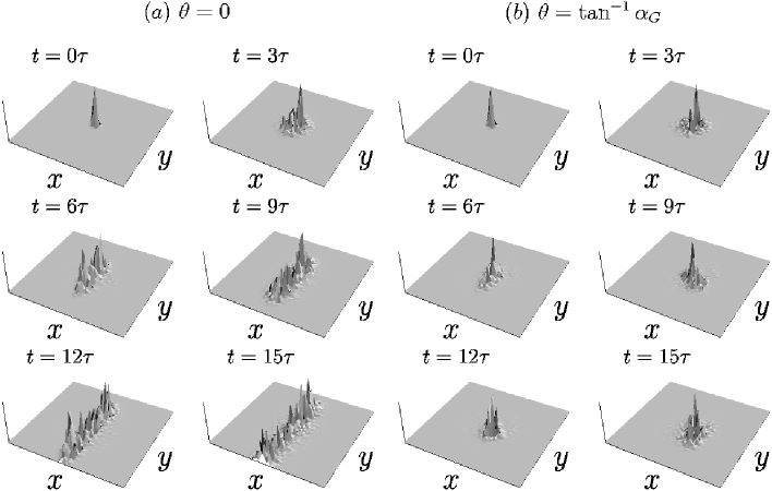
Figure 3: (a) Wave packet evolution when the electric field is oriented in an commensurate direction $\theta=0$, the electron is localized in the longitudinal direction. (b) Wave packet evolution when the electric field is oriented in an incommensurate direction $\theta=\tan^{-1}\alpha_{G},$ $\alpha_{G}=\left[(\sqrt{5}-1)/2\right]$. The wave packet is localized in both directions. In both examples $\lambda=1$, and $\rho=0.1$

(i) Let us first consider the simplest commensurate case $\theta=0$. The wave package spreads along the transverse direction, Fig. 3a. The mean square $\sigma_{x}^{2}$ presents small amplitude oscillations, while $\sigma_{y}^{2}$ shows a ballistic growing, Fig. 4a. (ii) Incommensurate orientation: $\theta=\tan^{-1}\alpha_{G}$. Fig. 3b clearly shows that the wave packet is dynamically localized in both directions, within a finite region of the lattice. In Fig. 4b it is shown that both $\sigma_{x}^{2}$ and $\sigma_{y}^{2}$ oscillate. It is interestig to compare the periods of these oscillations: the period of $\sigma^{2}_{x}$ is $T_{x}\approx 6.9\tau$ and $\sigma^{2}_{y}$ has a period $T_{y}\approx 11.2\tau$. The ratio of this two periods is similar to the golden ratio $T_{x}/T_{y}\sim E_{y}/E_{x}=(\sqrt{5}-1)/2$, which seems to be a consequence of the relation between the two components of the drift velocity $v_{D}=E\left(\sin\theta,-\cos\theta\right)/B$. Along the $x$ direction the electron will take a time $T_{x}=qa/v_{D}\sin\theta$ to reach the extreme of the unit cell, while on the $y$ axis we have $T_{y}=a/v_{D}\sin\theta$, giving the correct relation between the two periods. Each time the electron reaches the border of a unit cell it reflects showing an oscillation in the mean square dispersions. The oscillations are damped because of tunneling.

The comparison of the commensurate (Fig. 3a) with incommensurate (Fig. 3b) cases clearly shows the very different transport properties of the electron depending on the relative orientation of the electric field with respect to the lattice. The behavior of the Shanon entropy is consistent with these results (Fig. 4c), we observe that for small times the evolution of $S$ is common for both cases, however for $t\geq 3\tau$ the growth of $S(t)$ corresponding to the irrational orientation is considerable reduced as compared to the rational case.

Figure 4: (a) Time evolution of the $\sigma_{x}^{2}$ and $\sigma_{y}^{2}$ variances when the electric field is aligned in a commensurate direction $\theta=0$. (b) Time evolution of $\sigma_{x}^{2}$ and $\sigma_{y}^{2}$ for an incommensurate direction $\theta=\tan^{-1}\alpha_{G}$ of $\mathbf{E}$. In both examples $\lambda=1$, and $\rho=0.1$. For the rational orientation of $\mathbf{E}$ the electron is only localized in the longitudinal direction, whereas for $\theta=\tan^{-1}\alpha_{G}$ it is localized in both directions. (c) Time evolution for the Shannon entropy for the two orientations of $\mathbf{E}$.

The localization for incommensurate directions of the electric field can be understood with the following argument. For the electric field orientation $tan\,\theta=m_{2}/m_{1}$, the periodicity is preserved along the longitudinal and transverse direction but with an extended lattice of side dimensions $b=a\,\sqrt{m_{1}^{2}+m_{2}^{2}}$. If additionally, the number of flux quanta in each of the new unit cells is given by a rational number, $i.e.$ $\sigma^{-1}=b^{2}B/(h/e)=p/q$, then the electric-magnetic translation symmetries are preserved in the extended lattice of dimensions $q\,b\times b=q\,(m_{1}^{2}+m_{2}^{2})\,a^{2}$ [7, 8]. With the new conditions, the on-site energies of the original lattice are no longer the same, in order to coherently propagate the electron has to tunnel a distance proportional to the new lattice dimensions $q\,(m_{1}^{2}+m_{2}^{2})\,a^{2}$. Clearly as $m_{1}$ or $m_{2}$ increases the wave packet diffusion will be inhibited. For irrational orientations of the electric field, we can consider the rational approximant $tan\,\theta=m^{(n)}_{2}/m^{(n)}_{1}$, then the system becomes quasi-periodic and the electrons are not allowed to propagate coherently thus leading to localization.

We have analyzed the time evolution of electron wave packets in a two-dimensional periodic system in the presence of magnetic and electric fields. The dynamics is governed by the effective Hamiltonian in (7), which consistently includes the coupling between Landau levels as well as the periodic and external field contributions. The inclusion of an electric field (for commensurate orientations) yields localization in the longitudinal direction; propagation takes place along the transverse direction. This effect is a physical consequence of the quantization of the energy levels with respect to the longitudinal quasi-momentum. Transition from extended to localized states are observed as $\tan\,\theta$ changes from rational to irrational values. It is expected that these phenomena should be experimentally accessible using lateral superlattices on semiconductor heterostructures, for example by measuring assymetry effect on the magnetoresistance and Hall conductance as the electric field orientation with respect to the lattice axis is varied.

References

- [1] S. Aubry and C. Andre, Ann. Israel Phys. Soc. 3 (1980) 133.
- [2] P. G. Harper, Proc. Phys. Soc. A 68 (1955) 874.
- [3] A. Rau, Phys. Status Solidi B 69 (1975) K9.
- [4] R. Peierls, Z. Phys. 80 (1933) 763.
- [5] J. Zak, Phys. Rev. Lett. 79 (1997) 533.
- [6] D. R. Hofstadter, Phys. Rev. B 14 (1976) 2239.
- [7] A. Kunold and M. Torres, Phys. Rev. B 61 (2000) 9879.
- [8] A. Kunold and M. Torres, cond-mat/0311111 v1 (2003).
- [9] H. N. Nazareno and P. E. de Brito, Phys. Rev. B 64 (2001) 045112.
- [10] A. Barelli, J. Bellissard and F. Claro, Phys. Rev. Lett. 83 (1999) 5082.
- [11] T. Schlösser, K. Ensslin, J. P. Kotthaus and M. Holland, Europhys. Lett. 33 (1996) 683.
- [12] C. Albrecht, J. H. Smet, D. Weiss, K. von Klitzing, R. Hennig, M. Langenbuch, M. Suhrke, U. Rssler, V. Umansky and H. Schweizer”, Phys. Rev. Lett. 83 (1999) 2234.
- [13] C. Albrecht, J. H. Smet, K. von Klitzing, D. Weiss , V. Umansky and H. Schweizer, Phys. Rev. Lett. 86 (2001) 147.
- [14] N. Ashby and S.C. Miller, Phys. Rev. B 139 (1965) A428.
- [15] C. E. Shannon, Bell Syst. 109 (195) 1492.
- [16] R. Ketzmerick and K. Kruse and D. Springsguth and T. Geisel, Phys. Rev. Lett. 84 (2000) 2929.