Optimizing the ensemble for equilibration in broad-histogram Monte Carlo simulations

Abstract

We present an adaptive algorithm which optimizes the statistical-mechanical ensemble in a generalized broad-histogram Monte Carlo simulation to maximize the system’s rate of round trips in total energy. The scaling of the mean round-trip time from the ground state to the maximum entropy state for this local-update method is found to be $O([N\log N]^{2})$ for both the ferromagnetic and the fully frustrated 2D Ising model with $N$ spins. Our new algorithm thereby substantially outperforms flat-histogram methods such as the Wang-Landau algorithm.

I Introduction

At first-order phase transitions and in systems with many local minima of the free energy such as frustrated magnets or spin glasses, conventional Monte Carlo methods simulating canonical ensembles have very long equilibration times. Several simulation methods have been developed to speed up such systems, including the multicanonical method Multicanonical , broad histograms BroadHistograms , parallel tempering Tempering , the Wang-Landau algorithm WangLandau and variations thereof WLVariations . Most of these methods simulate a flat-histogram ensemble: Instead of sampling a configuration of energy $E$ with Boltzmann weight $w(E)\propto\exp(-\beta E)$, they use weights $w(E)\propto 1/g(E)$, where $g(E)$ is the density of states. The probability distribution of the energy, $n(E)=w(E)g(E)$, then becomes constant, producing a flat energy histogram. Naively, one might assume that sampling all energies equally often produces an unbiased random walk in energy. However, it was recently shown Limitations that the growth with the number of spins $N$ of the “tunneling times” between low and high energy in any local-update flat-histogram method is stronger than the naive $N^{2}$ of an unbiased random walk in energy for various 2D Ising models: as $\sim N^{2.4}$ for the ferromagnetic and $\sim N^{2.9}$ for the fully-frustrated models. For the 2D $\pm J$ spin glass, exponential growth was observed Limitations .

In view of these results for flat-histogram simulations Limitations we have asked how this type of simulation can be improved, both in terms of computer time and statistical errors. The general type of application we have in mind is to the equilibrium behavior of a system that is very slow to equilibrate in a conventional simulation, such as domain walls in ordered phases, low-energy configurations of frustrated systems or a spin-glass ordered phase. Our new algorithm instead simulates a broad-histogram ensemble, where the system can, at “equilibrium” in this ensemble, wander to part of its phase diagram where equilibration is rapid. We look specifically at histograms that are broad in energy, but in general another variable other than the energy could be used. To minimize the statistical errors of measurements in the energy range of interest, one maximizes the number of statistically-independent visits. For a glassy phase, the system will relax very little as long as it remains in that phase, so to get a new statistically-independent visit to the phase the system has to leave it and equilibrate elsewhere (usually at high energies). Thus the quantity we want our simulation to maximize is the number of round trips – between low and high energy – per unit computer time. This should minimize both the simulation’s equilibration time and the statistical errors in the low-energy regime of interest.

In this paper, we present an algorithm that systematically optimizes the ensemble simulated to maximize the rate of round trips in energy. We use a feedback loop that reweights the ensemble based on preceding measurements of the local diffusivity of the total energy. This detects the “bottlenecks” in the simulation as minima in the diffusivity (at critical points in the cases we study), and reallocates resources to those energies in order to minimize the slowdown. We find that the resulting statistical errors in the density of states as estimated by this new algorithm are nearly uniform in energy, in strong contrast to flat-histogram simulations where the errors are much larger at low energy than at high energy. While our algorithm is rather general and should be widely applicable to study complex systems, we have developed and tested it on ferromagnetic (FMI) and fully-frustrated (FFI) square-lattice Ising models.

II Feedback of local diffusivity

In our simulations, the system’s energy does a random walk in the energy range between two extremal energies, $E_{-}\leq E\leq E_{+}$ where we take the lowest energy $E_{-}$ to be the system’s ground state, although this is not necessary for our approach. Consider a general ensemble, with weights $w(E)$, which define the acceptance probabilities for moves based on the Metropolis scheme

$$p(E\rightarrow E^{\prime})=\min\left(1,\frac{w(E^{\prime})}{w(E)}\right)~{}.$$ (1)

Our algorithm iteratively collects data from batch runs which simulate with a fixed ensemble. During a simulation detailed balance is strictly satisfied at all times. For a reasonably large number of sweeps we can thus measure the equilibrium distribution of the energy in this ensemble which is $n_{w}(E)\propto w(E)g(E)$. The simulated system does a biased and Markovian random walk in configuration space. Since we bias this walk based only on total energy, the projection of this random walk onto that variable is what we will discuss. This projection, which ignores all properties of the state other than its total energy, results in a random walker that is non-Markovian, with its memory stored in the system’s configuration. Thus the simulation may be viewed as a biased non-Markovian random walker moving along the allowed energy range between the two extremal energies.

To measure the round trips we add a label to the walker that says which of the two extremal energies it has visited most recently. The two extrema act as “reflecting” and absorbing boundaries for the labeled walker: e.g., if the label is plus, a visit to $E_{+}$ does not change the label, so this is a “reflecting” boundary. However, a visit to $E_{-}$ does change the label, so the plus walker is absorbed at that boundary. The steady-state distributions of the labeled walkers satisfy $n_{-}(E)+n_{+}(E)=n_{w}(E)$. It is important to note that the behavior of the labeled walker is not affected by its label except when it visits one of the extrema and the label changes. When the unlabeled walker is at equilibrium, the labeled walker is in a nonequilibrium steady state. Let $f(E)=n_{+}(E)/n_{w}(E)$ be the fraction of the walkers at $E$ that have label plus, so they have most recently visited $E_{+}$. The above-discussed boundary conditions dictate $f(E_{-})=0$ and $f(E_{+})=1$.

To calculate the rate of round trips, we note that in steady state the current $j$ of the labeled walkers is independent of $E$. The plus and minus walkers drift in opposite directions and the equilibrium unlabeled walker has no net current. We first examine the case of a continuous energy $E$. The steady-state current from $E_{+}$ to $E_{-}$ to first order in the derivative is

$$j=D(E)n_{w}(E){{df}\over{dE}}~{},$$ (2)

where $D(E)$ is the walker’s diffusivity at energy $E$. There is no current if $f$ is constant, since this is equilibrium; this is why the current is to leading order proportional to $df/dE$. If one rearranges the above equation and integrates on both sides, noting that $j$ is a constant and $f$ runs from 0 to 1, one obtains

$${1\over{j}}=\int_{E_{-}}^{E_{+}}{{dE}\over{D(E)n_{w}(E)}}~{}.$$ (3)

In the following we separately discuss how we can maximize the rate of round-trips for Metropolis and $N$-fold way dynamics based on this estimate of the current.

II.1 Metropolis dynamics

For Metropolis dynamics the rate of round-trips is simply proportional to the current. To maximize the round-trip rate, the above integral, Eq. (3), must be minimized. However, there is a constraint: $n_{w}(E)$ is a probability distribution and must remain normalized. We do this by adding a Lagrange multiplier:

$$\int_{E_{-}}^{E_{+}}dE\left({1\over{D(E)n_{w}(E)}}+\lambda n_{w}(E)\right)~{}.$$ (4)

To minimize this integrand, the ensemble, that is the weights $w(E)$ and thus $n_{w}(E)$ are varied. At this point we assume that the dependence of $D(E)$ on the weights can be neglected. This is justified by noting that the rates of transitions between configurations depend only on the ratios of weights, so the diffusivity $D(E)$ is unchanged when the weights are multiplied by an energy-independent constant. By ignoring the variation of $D(E)$ with the weights, we are assuming that the adjustments to the weights are slowly-varying in energy, which is true for most systems, particularly for large systems where the energy range being studied is large. With this assumption, the optimal weighting which minimizes the above integrand is

$$n_{w}^{(opt)}={1\over{\sqrt{D(E)\lambda}}}={{df^{(opt)}}\over{dE}}~{}.$$ (5)

Thus for the optimal ensemble with Metropolis dynamics, the probability distribution is simply inversely proportional to the square root of the local diffusivity.

II.2 $N$-fold way dynamics

Since Metropolis dynamics can be slowed down by high rejection rates of singular moves, e.g. in the vicinity of the fully polarized ground state of the FMI, or the occurrence of multiple, generally accepted zero-energy moves it can be advantageous to introduce rejection-free single-spin flip updates such as the $N$-fold way NFoldWay . $N$-fold way dynamics involve two time scales, the walker’s time and the computer time. At a given energy level the two time scales differ by the (energy-dependent) lifetime of a given spin configuration. The random walk with $N$-fold way dynamics is an equilibrium process when measured in walker’s time, that is the equilibrium distribution, $n_{w}(E)$, is proportional to the amount of walker’s time the walker spends at $E$. However, for the ensemble optimization with $N$-fold way dynamics we want to speedup the random walk measured in computer time. This setup with two clocks requires a slightly different reweighting procedure than is presented above for Metropolis dynamics.

As for the Metropolis dynamics the amount of walker’s time it takes to make a round trip is proportional to $1/j$ given in Eq. (3). However, we are interested in minimizing the amount of computer time spent, so we need to multiply this by the ratio of computer time to walker’s time at $E$ which we denote as $t(E)$. Let us assume the distribution $n_{w}(E)$ is normalized to integrate to one. Then for one unit of walker’s time, the fraction spent at $E$ in $dE$ is $n_{w}(E)dE$. The amount of computer time used per unit walker’s time is thus

$$T=\int_{E_{-}}^{E_{+}}n_{w}(E)t(E)dE~{}.$$ (6)

To find the weights that minimize the round-trip time as measured in computer time, the full quantity we want to minimize is thus

$$\int_{E_{-}}^{E_{+}}{{dE}\over{D(E)n_{w}(E)}}\int_{E_{-}}^{E_{+}}t(E^{\prime})n_{w}(E^{\prime})dE^{\prime}~{}.$$ (7)

Since the probability distribution $n_{w}(E)$ occurs in both the numerator and denominator of the integrand there is no need to enforce its normalization by a Lagrange multiplier. To extremize the integrand, we will again vary the weights $w(E)$, which gives the following condition for the optimum:

$${{T}\over{D(E)n_{w}^{2}(E)}}={{t(E)}\over{j}}~{},$$ (8)

so the weights should be chosen to give the optimal distribution

$$n_{w}^{(opt)}(E)=\sqrt{{{jT}\over{D(E)t(E)}}}~{}.$$ (9)

For the optimal ensemble with $N$-fold way dynamics, the probability distribution is thus larger at the points with smaller $t(E)$ (since they do not cost a lot of computer time) and smaller diffusivity $D(E)$.

II.3 Feedback iteration

To feed back we simulate with some trial weights $w(E)$, get steady-state data for $n_{w}(E)$ and $f(E)$ and thus obtain estimates for the diffusivity via

$$D(E)={{j}\over{n_{w}(E){{df}\over{dE}}}}~{}.$$ (10)

For Metropolis dynamics chose new weights $w^{\prime}(E)$ so that

$$n_{w^{\prime}}(E)=A\sqrt{n_{w}(E){{df}\over{dE}}}~{},$$ (11)

where $A$ is a normalization constant whose value is not needed to run the next “batch” of the simulation with the new weights $w^{\prime}(E)$. For $N$-fold way dynamics the new weights $w^{\prime}(E)$ are chosen to be

$$n_{w^{\prime}}(E)=\sqrt{n_{w}(E){{df}\over{dE}}{T\over{t(E)}}}~{}.$$ (12)

In practice we work with the logarithms of the weights, so the reweighting becomes

$$\ln w^{\prime}(E) = \ln w(E)$$

$$+\frac{1}{2}\left(\ln\left\{{{df}\over{dE}}\right\}-\ln n_{w}(E)-\ln t(E)\right)\;,$$

where all energy independent terms have been dropped as they introduce a constant shift only. For Metropolis updates the last term $\ln t(E)$ can also be dropped. Each subsequent batch should be run significantly longer than the previous one – in our implementation we double the number of sweeps – in order to get better statistics, and fed back to improve the estimates of the optimal weights.

III Implementation and Applications

We implemented this algorithm for 2D Ising models with single-spin-flip Metropolis and $N$-fold way dynamics, found the optimal ensembles for the FMI and FFI models, obtained the scaling of round-trip times and calculated the density of states and its statistical errors for both models. In both cases we used the ground state, $E_{-}=E_{0}$, and zero energy, $E_{+}=0$, as the energy limits.

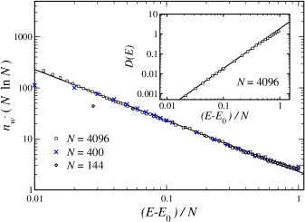
Figure 1: Histograms of the optimal ensemble for the 2D fully frustrated Ising model with Metropolis dynamics. For various system sizes and a broad energy range the rescaled data points collapse onto a a power-law divergence $[(E-E_{0})/N\ln N]^{-1}$ (bold line). The inset shows the diffusivity $D(E)$ for the same model which is proportional to $[(E-E_{0})/N]^{2}$ (bold line).

In the initial batch mode step we simulated a flat-histogram ensemble for small system sizes using either the exact density of states footnote or a rough estimate thereof calculated with the Wang-Landau algorithm WangLandau . For larger systems ($N>64\times 64$) where the round-trip times for the flat-histogram ensemble are more than a magnitude larger than for the optimized ensemble, we produced an initial estimate of the optimal weights by extrapolating the optimized weights of smaller systems. For all batch mode steps the fraction of labeled walkers, $f(E)$, was determined by recording two histograms, one for the equilibrium (unlabeled) walker and one for the labeled walker which most recently visited $E_{-}$. The derivative $df/dE$ was then estimated by a linear regression of several neighboring points at each energy level. The number of points used for the regression can be reduced for subsequent batch mode steps as the estimate of $f(E)$ becomes increasingly accurate due to better statistics. In the final batch mode steps of our calculations the regression was performed using a minimum of three points. In general, there is a trade-off between the accuracy in the measurement of the local diffusivity and the number of feedback steps. For the Ising models we study we found rapid convergence to the optimal ensemble. For small systems, $N\leq 32\times 32$, an initial batch mode step with some $10^{5}$ to $10^{6}$ sweeps was sufficient to find the optimal weights after the first feedback step. Since the possible energy levels are discrete for the Ising model, special care is taken when applying the reweighting derived for the continuum limit, particularly at the boundaries of the energy interval $[E_{-},E_{+}]$. However, we did not encounter any subtlety for either model.

III.1 Fully frustated Ising model

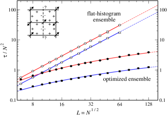
Figure 2: Scaling of round-trip times in the energy interval $[-N,0]$ for the flat-histogram (open symbols) and optimized ensemble (filled symbols) of the 2D fully frustrated Ising model with Metropolis (circles) and $N$-fold way (squares) dynamics. The solid lines correspond to a logarithmic (power-law) fit for the optimized (flat-histogram) ensemble. The inset illustrates the frustrated couplings of the fully frustrated model.

We first present our results for the fully-frustated model (FFI), which has a critical point at its ground state, and shows rather simple scaling of our algorithm’s behavior with energy and system size. For the optimized ensemble of the FFI the histogram of the equilibrium random walker is no longer flat, but exhibits a power-law divergence at its ground state, as shown in Fig. 1. This divergence reflects the behavior, $D(E)\sim[(E-E_{0})/N]^{2}$ of the diffusivity, as is seen in the inset of Fig. 1. These power-law behaviors extend from the first few points, $E-E_{0}=O(1)$, up nearly to zero energy, $E-E_{0}=O(N)$. If we accept that the critical exponent for the diffusivity is indeed 2, then the optimal distribution scales as $n_{w}\sim 1/[(E-E_{0})\ln N]$, and the round-trip time as $\tau\sim(N\ln N)^{2}$, consistent with our results shown in Figs. 1 and 2.

Noting that for our optimized ensemble the system spends a large fraction of its time near the ground state where many Metropolis moves are rejected, we applied a version of our algorithm that instead uses single-spin-flip rejection-free $N$-fold way updates. We find the $N$-fold way updates do give a significant speedup compared to Metropolis dynamics, but do not change the $\tau\sim(N\ln N)^{2}$ scaling of the round-trip time. In comparison to the performance of flat-histogram sampling we find a substantial speedup up to a factor of around $50$ for the largest simulated system with $N=128\times 128$ spins, see Fig. 2.

III.2 Ferromagnetic Ising model

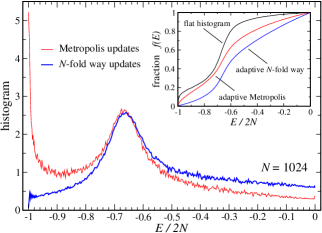
Figure 3: Histograms for the 2D ferromagnetic Ising model obtained after feedback: for the optimal ensemble a peak evolves around the critical energy in the histograms. The additional peak near the fully polarized groundstate found for Metropolis updates (thin line) can be eliminated by changing the dynamics to $N$-fold way updates (bold line). The inset shows the fraction $f(E)$ of walkers which have most recently visited $E_{+}=0$ for flat-histogram (multicanonical) sampling and the optimal ensembles for Metropolis and $N$-fold way dynamics.

We now turn to the results for the ferromagnetic Ising model (FMI) which exhibits a finite-temperature second order phase transition. After applying the feedback, we find a peak in the histogram near the critical energy, as shown in Fig. 3. For Metropolis updates a second divergence close to the fully polarized ground state appears which is eliminated by changing the dynamics to rejection-free $N$-fold way moves. However, the minimum in the diffusivity at the critical point remains with $N$-fold way dynamics and the resulting peak in the histogram is not suppressed. With increasing system size this power-law divergence moves towards the critical energy of the infinite system, $E_{c}/2N\cong-0.71$, as illustrated in the inset of Fig. 4. For both types of single-spin-flip moves we find that the rate of round trips between the magnetically ordered and disordered phases of the ferromagnet appear to scale as $\tau\sim(N\ln N)^{2}$ as for the FFI model, see Fig. 4.

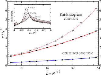
Figure 4: Scaling of round-trip times in the energy interval $[-2N,0]$ for the flat-histogram ensemble (open symbols) and the optimal ensemble (filled symbols) of the 2D ferromagnetic Ising model with Metropolis (circles) and $N$-fold way dynamics (squares). The solid (dashed) lines correspond to a logarithmic (power-law) fit for the optimized (flat-histogram) ensemble. The inset shows the scaling of histograms for the optimal ensemble for $N$-fold way updates.

IV Statistical errors

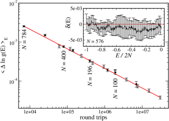
Figure 5: Average statistical error $\langle\Delta\ln g(E)\rangle_{E}$ of the computed density of states of the FFI model versus the number of round trips in the energy interval $[-N,0]$. The statistical errors were obtained for 16 independent runs and averaged over all energies for $N=36$ (open symbols). Data points for larger system sizes are superimposed (solid symbols), with the system size increasing from right to left. The statistical error reduces like $1/\sqrt{\mbox{round trips}}$ (solid line) for all system sizes. The inset shows the deviation, $\delta(E)=\ln g(E)-\ln g_{\mbox{exact}}(E)$, from the exact result for the $24\times 24$ FMI model obtained for 16 independent runs with $3.2\cdot 10^{6}$ sweeps.

Finally we address the statistical errors of measurements performed during the simulation. Standard tools can be used for the error analysis as the simulated random walk in configuration space is a conventional Markov chain Monte Carlo simulation. Only the projection of this random walk onto energy space becomes non-Markovian which is irrelevant for the measurements.

For each batch mode step simulating a fixed statistical ensemble $w(E)$ we can measure the density of states, $\ln g(E)=\ln n_{w}(E)-\ln w(E)$, from the recorded equilibrium distribution $n_{w}(E)$. Comparing our results with the exact density of states we find perfect agreement within the statistical errors as illustrated for the FMI in the inset of Fig. 5. The observed distribution of statistical errors is nearly flat in energy, which is a further improvement compared to flat-histogram simulations where the errors can be orders of magnitude larger at low energy than at high energy WangLandau . The statistical error is found to scale as $\Delta\ln g(E)\sim 1/\sqrt{\mbox{round trips}}$ with the number of round trips in energy which is shown in the main panel of Fig. 5. For different system sizes we find the statistical errors to collapse onto a single $1/\sqrt{\mbox{round trips}}$ dependence which a posteriori validates our goal of maximizing the rate of round trips.

V Conclusions

The presented algorithm should be widely applicable to study the equilibrium behavior of complex systems, such as glasses, dense fluids or polymers. To speed up the system’s equilibration the rate of round trips in energy is maximized by systematically optimizing the statistical ensemble based on measurements of the local diffusivity. We find that the relative statistical error in the density of states as calculated with the new method scales as $O(1/\sqrt{\mbox{round trips}})$. For the 2D ferromagnetic and fully frustrated Ising models the round-trip time from the ground state to the maximum entropy state scales like $O([N\log N]^{2})$ which is a significant speedup compared to the power law behavior $O(N^{2+z})$ of flat-histogram algorithms.

The idea of performing round-trips in energy is similar to the parallel tempering algorithm Tempering which simulates replicas of the system at various temperatures. The swapping of replicas at neighboring temperatures can be viewed as a random walk of the replicas along the temperature. In order to maximize the round-trips in temperature one can use our algorithm to systematically optimize the simulated temperature set which we will discuss in a forthcoming publication FutureTempering .

VI Acknowledgments

We thank S. Sabhapandit for providing the exact density of states for the FFI and R. H. Swendsen for helpful discussions. ST acknowledges support by the Swiss National Science Foundation. DAH is supported by the NSF through MRSEC grant DMR-0213706.

References

- (1) B. A. Berg and T. Neuhaus, Phys. Rev. Lett. 68, 9 (1992); Phys. Lett. B. 267, 249 (1991).
- (2) P. M. C. de Oliveira et al., Braz. J. Phys. 26, 677 (1996).
- (3) K. Hukushima and K. Nemoto, J. Phys. Soc. Japan 65, 1604 (1996); E. Marinari and G. Parisi, Europhys. Lett. 19, 451 (1992); A. P. Lyubartsev et al., J. Chem. Phys. 96, 1776 (1992).
- (4) F. Wang and D. P. Landau, Phys. Rev. Lett. 86, 2050 (2001a); Phys. Rev. E 64, 056101 (2001b).
- (5) Q. Yan and J. J. de Pablo, Phys. Rev. Lett. 90, 035701 (2003); M. S. Shell et al., J. Chem. Phys. 119, 9406 (2003); M. Troyer et al., Phys. Rev. Lett. 90, 120201 (2003); C. Zhou and R. N. Bhatt, cond-mat/0306711.
- (6) P. Dayal et al., Phys. Rev. Lett. 92, 097201 (2004).
- (7) A. B. Bortz et al., J. Comput. Phys. 17, 10 (1975).
- (8) The exact density of states was calculated with the algorithms Beale:96 and Saul:94 for the FMI (up to ) and FFI (up to ) respectively.
- (9) P. D. Beale, Phys. Rev. Lett. 76, 78 (1995).
- (10) L. K. Saul and M. Kardar, Nuclear Physics B 432, 641 (1994).
- (11) D. A. Huse, H. G. Katzgraber, S. Trebst, M. Troyer, in preparation