Elongation and fluctuations of semi-flexible polymers in a nematic solvent

Abstract

We directly visualize single polymers with persistence lengths ranging from $\ell_{p}=0.05$ to $16$ $\mu$m, dissolved in the nematic phase of rod-like fd virus. Polymers with sufficiently large persistence length undergo a coil-rod transition at the isotropic-nematic transition of the background solvent. We quantitatively analyze the transverse fluctuations of semi-flexible polymers and show that at long wavelengths they are driven by the fluctuating nematic background. We extract both the Odijk deflection length and the elastic constant of the background nematic phase from the data.

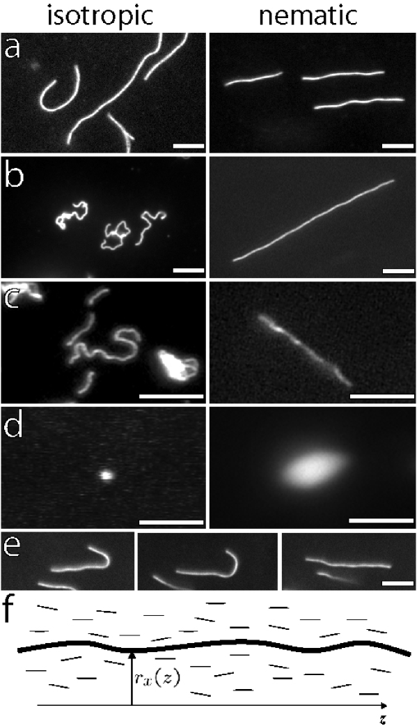
Figure 1: Images of fluorescently labelled biopolymers in the isotropic (left) and nematic (right) phase of fd virus. Figures (a)-(d) are, respectively, the images of actin, wormlike micelles, neurofilaments, and DNA. The polymers in an isotropic solution are confined by a thin chamber thus making the samples quasi two dimensional. (e) A sequence of images illustrating an actin filament escaping from a hairpin defect. The scale bar is 5 $\mu$m. (f) A schematic of a biopolymer in the background nematic field; the conformation of the polymer is parameterized by ${\bf R}(z)=\left\{\,r_{x}(z),r_{y}(z),z\right\}$. The nematic director points along the $z$-axis.

Polymer coils in solution exhibit a variety of conformational and dynamical behaviors depending on many factors, including polymer concentration, polymer stiffness, solvent quality, solvent flow, and mechanical stress. Exciting recent experiments in this field have focused on disentanglement of single biopolymers in isotropic solutions as a result of applied forces and solvent flow chu and on transport of single biopolymers through networks of barriers craighead , which is critically affected by conformational dynamics of the polymers. In this Letter, we explore conformations of polymer coils in anisotropic solutions. In particular, we present the first direct experimental observations of isolated semi-flexible polymers dissolved in a background nematic phase composed of aligned rod-like macromolecules. We show by direct visualization that semi-flexible biopolymers dissolved in the nematic phase assume an elongated rod-like configuration aligned with the background nematic director. The coil-rod transition of the biopolymer can thus be induced by causing the solvent to undergo an isotropic-to-nematic (I-N) transition by increasing the concentration of its constituent rods. We quantitatively explore the fluctuations of these semi-flexible polymers and find they cannot be described by a theory which treats the nematic background as a fixed external field warner .

Mixtures of semi-flexible polymers in lyotropic nematic suspensions exemplify an emerging class of complex fluids – hyper-complex fluids, for example nematic elastomers Warner and nematic emulsions Weitz , wherein two or more distinct components are combined to create systems that exhibit novel physical properties and functions. Understanding the polymer-nematic system may lead to new ideas about how to achieve high alignment of biopolymers that is complementary to existing methods of DNA alignment BenNama02 . Furthermore, since many biopolymers such as the actin filaments within the sarcomere and neurofilaments within the axon reside in an anisotropic, nematic-like environment Aldoroty , our investigation may shed light on organization mechanisms within the cell.

We have used fluorescence microscopy to study four different biopolymers in isotropic and nematic colloidal suspensions. This approach yields new information about dynamics and defects not readily accessible to traditional probes such as x-ray or neutron scattering xray . In addition, we have developed a rotationally-invariant free energy for a single semiflexible polymer in a nematic matrix which generalizes the work in deGennes82 ; Kamien92 , and enables us to extract the Odijk length Odijk86 and the elastic constant of the liquid crystal. These first direct measurements of the Odijk deflection length, $\lambda$, allow us to quantify the length scale over which the polymer wanders before it is deflected back by the nematic director.

Table 1: The contour length $L$, the persistence length $\ell_{p}$, and the diameter $a$ of bio-polymers in our experiments.

Polymer	$L$ [$\mu$m]	$\ell_{p}$ [$\mu$m]	$a$ [nm]	Ref.
$\lambda$-DNA	16	0.05	2	Wang97
neurofilament	2-10	0.2	10	Aranda03
wormlike micelles	5-50	0.5	14	Won99
F-actin	2-20	16	7	actin
fd virus	0.9	2.2	7	Dogic01

Our experiments employ an aqueous solution of rod-like fd viruses as a background nematic liquid crystal. This system has been studied extensively Tang ; Dogic01 ; Purdy03 , and its phase behavior is well described by the Onsager theory for rods with hard core repulsion Onsager49 . Another advantage of this system is its compatibility with most biopolymers. We use four different semi-flexible polymers, whose physical parameters are listed in Table 1. To directly visualize the polymers dissolved in the nematic background, we fluorescently labelled each polymer: DNA was labelled with YOYO-1 (Molecular Probes, Eugene OR), neurofilaments with succinimidyl rhodamine B Leterrier96 , F-actin filaments with rhodamine-phalloidin (Sigma, St. Louis MO), and wormlike micelles with PKH26 dye (Sigma, St. Louis MO) which preferentially partitions into the hydrophobic core of the micelle. Since DNA, neurofilaments, and actin are all negatively charged, we expect that they are stable in a suspension of negatively charged fd viruses. Wormlike micelles are sterically stabilized with a neutral PEO brush layer, which does not interact with fd virus or other proteins Won99 ; Dogic01 .

Bacteriophage fd was grown and dialyzed against a phosphate buffer (150 mM KCl, 20 mM phosphate, 2 mM MgCl₂, pH=7.0) Dogic01 . Samples were prepared by mixing a small amount of polymer with fd solution at different concentrations and were placed between a coverslip and a glass slide. A chamber with a thickness of $\sim 50\,\mu$m was made by using a stretched parafilm as a spacer. Samples sealed with optical glue (Norland Products, Cranbury, NJ) were allowed to equilibrate until no drift was visually detectable. To reduce photobleaching, we added anti-oxygen solution ($2$ mg/ml glucose, $360$ U/ml catalase, 0.25 vol$\%$ mercaptoethanol, 8 U/ml glucose oxidase). All samples were imaged with a fluorescence microscope (Leica IRBE) equipped with a 100x oil-immersion objective and a $100$ W mercury lamp. Images were taken with a cooled CCD camera (CoolSnap HQ, Roper Scientific), which was focused at least 5 $\mu$m away from the surface to minimize possible wall effects.

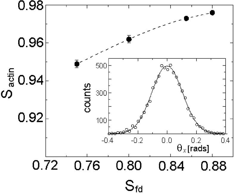
Figure 2: The order parameter of actin filaments ($S_{actin}$) vs. the order parameter of the background fd nematic ($S_{fd}$). Dashed line is a guide to the eye. The contour length of actin filaments is 15 $\mu$m or higher. The values of $S_{fd}$ at different fd concentration have been measured in Ref. Purdy03 . Inset: The orientational distribution function (ODF) of actin filaments. The ODF is well approximated by a Gaussian distribution for a wide range of concentrations.

Figure 1 displays a series of pictures that summarize our qualitative observations. In the nematic phase of $fd$, F-actin (Fig. 1a), wormlike micelles (Fig. 1b), and neurofilaments (Fig. 1c) are highly elongated, having a rod-like shape. By contrast, the same filaments dissolved in an isotropic phase crumple into more compact random coils. Just above the I-N transition, actin filaments and worm-like micelles form hairpin defects deGennes82 . These hairpins exhibit interesting dynamics as shown in Fig. 1e, and will be explored by us in detail elsewhere. DNA dissolved in fd nematic behaves qualitatively differently (Fig. 1d); it forms a slightly anisotropic droplet. Each droplet contains many DNA molecules and, with time, these droplets coalesce into a larger droplet. Thus, even at a very low concentration, DNA separates from the fd nematic. Taken together, these observations suggest that the persistence length of the polymer is important in determining its solubility in the nematic liquid crystals: DNA has a small $\ell_{p}$ and is insoluble, unlike the other stiffer polymers in our experiments. This insolubility may be related to the entropy-driven phase-separation of a system of bidisperse rigid rods if their lengths and/or diameters are sufficiently dissimilar Roij96c . This theory, however, has not been extended to the case of semi-flexible polymers.

The large contour lengths of actin filaments and wormlike micelles make them suitable for further quantitative analysis. We focus on the fluctuations of filaments in a background nematic that is free of both defects and distortions. A series of 50 to 100 images where taken with a few seconds between each image to ensure that statistically independent configurations were sampled. For each fd concentration, ten filaments were analyzed. The conformation of each polymer was reconstructed by manually marking the end points. (Note that we parameterize the transverse deviations of the polymer from the $z$ axis by the 2-component vector ${\bf r}(z)$, as shown in Fig. 1f.) An intensity profile along the $x$ direction for each value of $z$ was extracted. By fitting this intensity to a Gaussian, we obtained sub-pixel accuracy for $r_{x}(z)$. We first extracted the orientational distribution function (ODF) from our data. Since our images are two dimensional projections of the polymer fluctuating in three dimensions, the $x$-component of the tangent vector is measured by $t_{x}(z)=\partial\,r_{x}(z)/\partial z\approx\theta_{x}(z)$. The ODF is obtained by creating a histogram of $\theta_{x}$ at different positions along the contour length for a time sequence of 50-100 images. A typical ODF is plotted in Fig. 2a; it is well approximated by a Gaussian distribution.

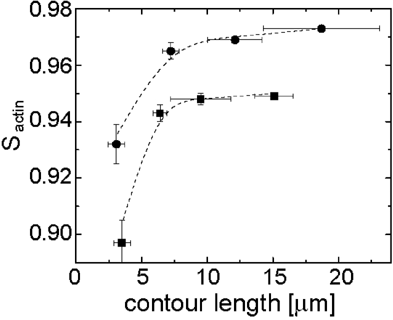
Figure 3: $S_{actin}$ vs. contour lengths of actin. The concentrations of the background nematic fd are 41 mg/ml (squares, $S_{fd}=0.75$) and 28 mg/ml (circles, $S_{fd}=0.855$). Dashed lines are a guide to the eye.

Next, we compute the order parameter of the polymer defined by: $S\equiv\int_{0}^{L}\,dz\,\langle\,3\,({\bf t}(z)\cdot\hat{z})^{2}-1\,\rangle/(2L)=1-3\,\langle\,t_{x}^{2}(0)\,\rangle,$ where in the last equality, we have used $\langle\,t_{x}^{2}(z)\,\rangle=\langle\,t_{y}^{2}(z)\,\rangle$. In Fig. 2, we plot $S$ for actin as a function of the background nematic order parameter. It is interesting to observe that $S_{actin}$ is significantly higher than $S_{fd}$. In order to check that the difference in the alignment between actin and fd molecules is due to their different contour lengths, we measured $S_{actin}$ for different contour lengths of actin filaments, as shown in Fig. 3. As the contour length of actin decreases, $S_{actin}$ approaches $S_{fd}$, as expected intuitively. These observations are qualitatively consistent with the Onsager theory for a bidisperse mixture of rod-like particles with different lengths considered in Ref. Lekkerkerker84 . This theory predicts the order parameter of long rods will be higher than the order parameter of the background nematic of shorter rods.

Finally, we measured the tangent-tangent correlation function (TTCF) $\langle\,t_{x}(z^{\prime})\,t_{x}(z^{\prime}+z)\,\rangle$ for wormlike micelles dissolved in fd virus with concentration 40 mg/ml and above (Fig. 4). At low fd concentrations, the fluctuations of worms are large as evidenced by visual observation of spontaneous formation and dissolution of hairpin defects. In this regime, the measured TTCF does not decay uniformly. We thus focus our analysis on the regime where the background order parameter is very high, and the amplitude of the polymer fluctuations is small. This makes our data suitable for comparison with the theoretical model outlined below.

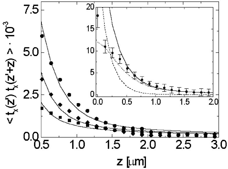
Figure 4: The $x$ component of the tangent-tangent correlation function for wormlike micelles measured at three different fd concentrations ($c_{fd}$). With increasing fd concentration the magnitude of the correlation function decreases. The solid lines are theoretical curves generated from Eq. (2) with the best-fit parameters listed in Table 2. Inset: TTCF for the lowest concentration of the fd virus. The dashed and dotted lines are respectively the contributions of the first and second term in Eq. (2). The data points below 0.5 $\mu$m are unreliable and have been excluded from the fitting fudge .

The fluctuations of a semi-flexible polymer in a nematic phase may be described by the free energy Kamien92 ; Selinger :

$$F = {k_{B}T\over 2}\int^{L}_{0}\,dz\left\{\ell_{p}\left[\,\frac{\partial{\bf t}_{\bot}}{\partial z}\,\right]^{2}+\Gamma\left[\,{\bf t}_{\bot}(z)-\delta{\bf n}(0,z)\,\right]^{2}\right\}$$ (1)

$$+ \frac{1}{2}\int d^{3}x\,K\,({\nabla}\delta{\bf n})^{2},$$

where $k_{B}$ is the Boltzmann constant, $T$ is the temperature, $\ell_{p}$ is the persistence length of the semi-flexible polymer, $\Gamma$ is the strength of the coupling of the polymer to the background nematic field, $\delta{\bf n}$ is the local direction of the fluctuating nematic field, and $K$ is the nematic elastic constant. Note that ${\bf t}_{\bot}$ and $\delta{\bf n}$ are two-dimensional vectors in the plane perpendicular to the average director. It is straightforward to compute $\langle\,t_{x}(z^{\prime})\,t_{x}(z^{\prime}+z)\,\rangle$ from Eq. (1):

$$\langle\,t_{x}(z^{\prime})\,t_{x}(z^{\prime}+z)\,\rangle=\frac{\lambda}{4\ell_{p}}\,e^{-z/\lambda}+\frac{1}{8\pi^{2}K\lambda}$$ (2)

$$\times\int_{0}^{\infty}dx\,\frac{\cos(xz/\lambda)\log(1+{D^{2}/x^{2}})}{(1+x^{2})\left[1+x^{2}+\frac{\Gamma x^{2}}{4\pi K}\,\log(1+{D^{2}/x^{2}})\right]},$$

where $D=2\pi\lambda/a$ is related to the molecular cutoff which we assume to be the diameter of the polymer ($a\sim 10$ nm). The first term in Eq. (2) describes the fluctuations of a semi-flexible polymer in a static external field, with a decaying length set by $\lambda=\sqrt{\ell_{p}/\Gamma}$. The second term describes the fluctuations of the polymers driven by the tight coupling to the fluctuations of the background nematic field. Note that this term generalizes that of Ref. Kamien92 , in that it includes the back reaction of the stiff polymer on the nematic fluctuations. Since it decays approximately as a power law, we expect at large lengthscales the fluctuations of the polymer are always dominated by the nematic fluctuations.

Figure 4 shows our measured TTCF along with the fitted curve of Eq. (2). Overall, good agreement is obtained at distances above 0.5 $\mu$m fudge . At these distances, most of the fluctuations of the worms are driven by the tight coupling to the background nematic field, coming from the second term in Eq. (2). The best-fit value of $\ell_{p}$ is found to be $1.5\,\mu$m, somewhat higher than that obtained in previous measurements Won99 . From the fits to the data, we extract the values of the Odijk deflection length $\lambda$, $K$, and $\Gamma$, as listed in Table 2. We observe that with increasing fd concentration, $\lambda$ decreases, while $K$ and $\Gamma$ increase, as one would intuitively expect. Finally, we note that the values for $K$ are in agreement with previous measurements of twist elastic constant $K_{22}=3\cdot 10^{-8}$ dyne for fd samples prepared under similar conditions Dogic00c .

Table 2: The Odijk deflection length $\lambda$, the elastic constant of the background nematic $K$, and the coupling constant between wormlike micelles and background nematic $\Gamma$ for different fd concentrations obtained from the fits shown in Fig. 4. The best-fit value of $\ell_{p}$ of wormlike micelles is 1.5 $\mu m$.

$c_{fd}$ [mg/ml]	$\lambda$ [$\mu$m]	$K$ [$10^{-8}$ dyne]	$\Gamma$ [1/$\mu$m]
39	0.18	1.9	46
51	0.13	2.4	88
97	0.06	2.8	416

In conclusion, we have shown that semi-flexible polymers with large enough persistence lengths assume a rod-like conformation when dissolved in a nematic solvent. Using image analysis, a full nematic orientational distribution function was measured. In addition, we have shown that fluctuations of the polymer are driven primarily by the fluctuations of the background nematic field. Direct visualization of individual polymer yields valuable new information about the behavior of polymer chains in anisotropic solvents.

This work was supported by the NSF through grant DMR-0203378 (AGY), DMR01-29804 (RDK), and the MRSEC Grant DMR-0079909, and from NASA NAG8-2172 (AGY), the NIH R01 HL67286 (PAJ), and the Donors of the Petroleum Research Fund, administered by the American Chemical Society (RDK).

References

- (1) T.T. Perkins et al., Science 268, 83 (1995); D.E. Smith et al., Science 283, 1724 (1999); C.M. Schroeder et al., Science 301, 1515 (2003); C. Bustamante et al., Nature 421, 423 (2003).
- (2) J. Han and H.G. Craighead, Science 288, 1026 (2000); D. Nykypanchuk et al., Science 297, 987 (2002).
- (3) M. Warner et al., J. Phys. A 18, 3007 (1985).
- (4) H. Finkelmann et al., Phy. Rev. Lett. 87, 015501 (2001).
- (5) P. Poulin et al., Science 275, 1770 (1997).
- (6) A. Bensimon et al., Science 265, 2096 (1994); V. Namasivayam et al., Anal. Chem. 74, 3378 (2002).
- (7) R.A. Aldoroty et al., Biophys. J. 51, 371 (1987); N. Hirokawa et al., J. Cell. Biol. 98, 1523 (1984).
- (8) X.L. Ao and R.B. Meyer, Physica A 176, 63 (1991); M.H. Li et al., Phys. Rev. Lett. 70, 2297 (1993); J.P. Cotton and F. Hardouin, Prog. Poly. Sci. 22, 795 (1997).
- (9) P.-G. deGennes, in Polymer Liquid Crystals, edited by A. Ciferri, W.R. Krigbaum, and R.B. Meyer (Academic, New York, 1982).
- (10) R.D. Kamien et al., Phys. Rev. A 45, 8728 (1992); Phys. Rev. E 48, 4119 (1993); P. LeDoussal and D.R. Nelson, Europhys. Lett. 15, 161 (1992).
- (11) T. Odijk, Macromolecules 19, 2313 (1986).
- (12) J. Tang and S. Fraden, Liquid Crystals 19, 459 (1995).
- (13) Z. Dogic and S. Fraden, Phil. Trans. R. Soc. Lond. A 359, 997 (2001).
- (14) K.R. Purdy et al., Phys. Rev. E 67, 031708 (2003).
- (15) L. Onsager, Ann. N.Y. Acad. Sci. 51, 627 (1949).
- (16) J. F. Leterrier et. al., J. Biol. Chem. 271, 15687, (1996).
- (17) P. Dalhaimer et al., Macromolecules 36, 6873 (2003).
- (18) M.D. Wang et al., Biophys. J. 72, 1335 (1997).
- (19) H. Aranda-Espinoza et al., to be published.
- (20) A. Ott et al., Phys. Rev. E. 48, 1642 (1993); F. Gittes et al., J. Cell. Biol. 120, 923 (1993).
- (21) R. van Roij and B. Mulder, J. Chem. Phys. 105, 11237 (1996).
- (22) H.N.W. Lekkerkerker et al., J. Chem. Phys. 80, 3427 (1984).
- (23) J.V. Selinger and R.F. Bruinsma, Phys. Rev. A. 43, 2910 (1991).
- (24) At distances smaller than 0.5 m, we observe a significant deviation of our data from the theoretical curve, which likely arises from the limited spatiotemporal resolution of our microscope. Over the image acquisition time of 250 ms, the fast fluctuations of the polymers at short wavelengths are effectively washed out, leading a lower value in the TTCF. Another possible source of discrepancy is that the spatial resolution of the microscope is smaller than the Odijk deflection length.
- (25) Z. Dogic and S. Fraden, Langmuir 16, 7820 (2000).